Transformers documentation
Performance and Scalability: How To Fit a Bigger Model and Train It Faster
Performance and Scalability: How To Fit a Bigger Model and Train It Faster
For now the software sections of this document are mainly Pytorch-specific, but the guide can be extended to other frameworks in the future.
Quick notes
This section gives brief ideas on how to make training faster and support bigger models. Later sections will expand, demonstrate and elucidate each of these.
Faster Training
Hardware:
- fast connectivity between GPUs
- intra-node: NVLink
- inter-node: Infiniband / Intel OPA
Software:
- Data Parallel / Distributed Data Parallel
- fp16 (autocast caching)
Bigger Models
Hardware:
- bigger GPUs
- more GPUs
- more CPU and NVMe (offloaded to by DeepSpeed)
Software:
- Deepspeed ZeRO
- Deepspeed ZeRO-Offload
- Megatron-LM 3D Parallelism
- Pipeline Parallelism
- Tensor Parallelism
- Low-memory Optimizers
- fp16/bf16 (smaller data/faster throughput)
- tf32 (faster throughput)
- Gradient checkpointing
- Sparsity
Hardware
Multi-GPU Connectivity
If you use multiple GPUs the way cards are inter-connected can have a huge impact on the total training time.
If the GPUs are on the same physical node, you can run:
nvidia-smi topo -mand it will tell you how the GPUs are inter-connected.
On a machine with dual-GPU and which are connected with NVLink, you will most likely see something like:
        GPU0    GPU1    CPU Affinity    NUMA Affinity
GPU0     X      NV2     0-23            N/A
GPU1    NV2      X      0-23            N/A
on a different machine w/o NVLink we may see:
        GPU0    GPU1    CPU Affinity    NUMA Affinity
GPU0     X      PHB     0-11            N/A
GPU1    PHB      X      0-11            N/A
The report includes this legend:
  X    = Self
  SYS  = Connection traversing PCIe as well as the SMP interconnect between NUMA nodes (e.g., QPI/UPI)
  NODE = Connection traversing PCIe as well as the interconnect between PCIe Host Bridges within a NUMA node
  PHB  = Connection traversing PCIe as well as a PCIe Host Bridge (typically the CPU)
  PXB  = Connection traversing multiple PCIe bridges (without traversing the PCIe Host Bridge)
  PIX  = Connection traversing at most a single PCIe bridge
  NV#  = Connection traversing a bonded set of # NVLinks
So the first report NV2 tells us the GPUs are interconnected with 2 NVLinks, and the second report PHB we have a typical consumer-level PCIe+Bridge setup.
Check what type of connectivity you have on your setup. Some of these will make the communication between cards faster (e.g. NVLink), others slower (e.g. PHB).
Depending on the type of scalability solution used, the connectivity speed could have a major or a minor impact. If the GPUs need to sync rarely, as in DDP, the impact of a slower connection will be less significant. If the GPUs need to send messages to each other often, as in ZeRO-DP, then faster connectivity becomes super important to achieve faster training.
NVlink
NVLink is a wire-based serial multi-lane near-range communications link developed by Nvidia.
Each new generation provides a faster bandwidth, e.g. here is a quote from Nvidia Ampere GA102 GPU Architecture:
Third-Generation NVLink® GA102 GPUs utilize NVIDIA’s third-generation NVLink interface, which includes four x4 links, with each link providing 14.0625 GB/sec bandwidth in each direction between two GPUs. Four links provide 56.25 GB/sec bandwidth in each direction, and 112.5 GB/sec total bandwidth between two GPUs. Two RTX 3090 GPUs can be connected together for SLI using NVLink. (Note that 3-Way and 4-Way SLI configurations are not supported.)
So the higher X you get in the report of NVX in the output of nvidia-smi topo -m the better. The generation will depend on your GPU architecture.
Let’s compare the execution of a gpt2 language model training over a small sample of wikitext.
The results are:
| NVlink | Time |
|---|---|
| Y | 101s |
| N | 131s |
You can see that NVLink completes the training ~23% faster.
In the second benchmark we use NCCL_P2P_DISABLE=1 to tell the GPUs not to use NVLink.
Here is the full benchmark code and outputs:
# DDP w/ NVLink

rm -r /tmp/test-clm; CUDA_VISIBLE_DEVICES=0,1 python -m torch.distributed.launch \
--nproc_per_node 2 examples/pytorch/language-modeling/run_clm.py --model_name_or_path gpt2 \
--dataset_name wikitext --dataset_config_name wikitext-2-raw-v1 --do_train \
--output_dir /tmp/test-clm --per_device_train_batch_size 4 --max_steps 200

{'train_runtime': 101.9003, 'train_samples_per_second': 1.963, 'epoch': 0.69}

# DDP w/o NVLink

rm -r /tmp/test-clm; CUDA_VISIBLE_DEVICES=0,1 NCCL_P2P_DISABLE=1 python -m torch.distributed.launch \
--nproc_per_node 2 examples/pytorch/language-modeling/run_clm.py --model_name_or_path gpt2 \
--dataset_name wikitext --dataset_config_name wikitext-2-raw-v1 --do_train
--output_dir /tmp/test-clm --per_device_train_batch_size 4 --max_steps 200

{'train_runtime': 131.4367, 'train_samples_per_second': 1.522, 'epoch': 0.69}
Hardware: 2x TITAN RTX 24GB each + NVlink with 2 NVLinks (NV2 in nvidia-smi topo -m)
Software: pytorch-1.8-to-be + cuda-11.0 / transformers==4.3.0.dev0
Software
Anatomy of Model's Operations
Transformers architecture includes 3 main groups of operations grouped below by compute-intensity.
Tensor Contractions
Linear layers and components of Multi-Head Attention all do batched matrix-matrix multiplications. These operations are the most compute-intensive part of training a transformer.
Statistical Normalizations
Softmax and layer normalization are less compute-intensive than tensor contractions, and involve one or more reduction operations, the result of which is then applied via a map.
Element-wise Operators
These are the remaining operators: biases, dropout, activations, and residual connections. These are the least compute-intensive operations.
This knowledge can be helpful to know when analyzing performance bottlenecks.
This summary is derived from Data Movement Is All You Need: A Case Study on Optimizing Transformers 2020
Anatomy of Model's Memory
The components on GPU memory are the following:
- model weights
- optimizer states
- gradients
- forward activations saved for gradient computation
- temporary buffers
- functionality-specific memory
A typical model trained in mixed precision with AdamW requires 18 bytes per model parameter plus activation memory.
For inference there are no optimizer states and gradients, so we can subtract those. And thus we end up with 6 bytes per model parameter for mixed precision inference, plus activation memory.
Let’s look at the details.
Model Weights
- 4 bytes * number of parameters for fp32 training
- 6 bytes * number of parameters for mixed precision training
Optimizer States
- 8 bytes * number of parameters for normal AdamW (maintains 2 states)
- 2 bytes * number of parameters for 8-bit AdamW optimizers like bitsandbytes
- 4 bytes * number of parameters for optimizers like SGD (maintains only 1 state)
Gradients
- 4 bytes * number of parameters for either fp32 or mixed precision training
Forward Activations
- size depends on many factors, the key ones being sequence length, hidden size and batch size.
There are the input and output that are being passed and returned by the forward and the backward functions and the forward activations saved for gradient computation.
Temporary Memory
Additionally there are all kinds of temporary variables which get released once the calculation is done, but in the moment these could require additional memory and could push to OOM. Therefore when coding it’s crucial to think strategically about such temporary variables and sometimes to explicitly free those as soon as they are no longer needed.
Functionality-specific memory
Then your software could have special memory needs. For example, when generating text using beam search, the software needs to maintain multiple copies of inputs and outputs.
forward vs backward Execution Speed
For convolutions and linear layers there are 2x flops in the backward compared to the forward, which generally translates into ~2x slower (sometimes more, because sizes in the backward tend to be more awkward). Activations are usually bandwidth-limited, and it’s typical for an activation to have to read more data in the backward than in the forward (e.g. activation forward reads once, writes once, activation backward reads twice, gradOutput and output of the forward, and writes once, gradInput).
Floating Data Types
Here are the commonly used floating point data types choice of which impacts both memory usage and throughput:
- fp32 (
float32) - fp16 (
float16) - bf16 (
bfloat16) - tf32 (CUDA internal data type)
Here is a diagram that shows how these data types correlate to each other.
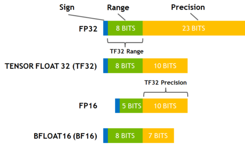
(source: NVIDIA Blog)
While fp16 and fp32 have been around for quite some time, bf16 and tf32 are only available on the Ampere architecture GPUS. TPUs support bf16 as well.
fp16
AMP = Automatic Mixed Precision
If we look at what’s happening with FP16 training (mixed precision) we have:
- the model has two copies in memory: one in half-precision for the forward/backward computations and one in full precision - no memory saved here
- the forward activations saved for gradient computation are in half-precision - memory is saved here
- the gradients are computed in half-precision but converted to full-precision for the update, no saving there
- the optimizer states are in full precision as all the updates are done in full-precision
So the savings only happen for the forward activations saved for the backward computation, and there is a slight overhead because the model weights are stored both in half- and full-precision.
In 🤗 Transformers fp16 mixed precision is enabled by passing --fp16 to the 🤗 Trainer.
Now let’s look at a simple text-classification fine-tuning on 2 GPUs (I’m giving the command for reference):
export BS=16
python -m torch.distributed.launch \
    --nproc_per_node 2 examples/pytorch/text-classification/run_glue.py \
    --model_name_or_path bert-base-cased \
    --task_name mrpc \
    --do_train \
    --do_eval \
    --max_seq_length 128 \
    --per_device_train_batch_size $BS \
    --learning_rate 2e-5 \
    --num_train_epochs 3.0 \
    --output_dir /tmp/mrpc \
    --overwrite_output_dir \
    --fp16
Since the only savings we get are in the model activations saved for the backward passed, it’s logical that the bigger those activations are, the bigger the saving will be. If we try different batch sizes, I indeed get (this is with nvidia-smi so not completely reliable as said above but it will be a fair comparison):
| batch size | w/o —fp16 | w/ —fp16 | savings |
|---|---|---|---|
| 8 | 4247 | 4163 | 84 |
| 16 | 4971 | 4793 | 178 |
| 32 | 6827 | 6207 | 620 |
| 64 | 10037 | 8061 | 1976 |
So there is only a real memory saving if we train at a high batch size (and it’s not half) and at batch sizes lower than 8, you actually get a bigger memory footprint (because of the overhead mentioned above). The gain for FP16 training is that in each of those cases, the training with the flag --fp16 is twice as fast, which does require every tensor to have every dimension be a multiple of 8 (examples pad the tensors to a sequence length that is a multiple of 8).
Summary: FP16 with apex or AMP will only give you some memory savings with a reasonably high batch size.
Additionally, under mixed precision when possible, it’s important that the batch size is a multiple of 8 to efficiently use tensor cores.
Note that in some situations the speed up can be as big as 5x when using mixed precision. e.g. we have observed that while using Megatron-Deepspeed.
Some amazing tutorials to read on mixed precision:
- @sgugger wrote a great explanation of mixed precision here
- Aleksey Bilogur’s A developer-friendly guide to mixed precision training with PyTorch
fp16 caching
pytorch autocast which performs AMP include a caching feature, which speed things up by caching fp16-converted values. Here is the full description from this comment:
Autocast maintains a cache of the FP16 casts of model parameters (leaves). This helps streamline parameter reuse: if the same FP32 param is used in several different FP16list ops, like several matmuls, instead of re-casting the param to FP16 on entering each matmul, the cast will occur on the first matmul, the casted FP16 copy will be cached, and for all later matmuls the FP16 copy will be reused. The cache is maintained only within a particular outermost autocast context. When you exit the autocast context the cache is dropped. For recommended usage, in which autocast wraps the forward pass, and then you exit the context before calling backward(), this means the cache only lasts the duration of the forward pass each iteration, and will be rebuilt next iteration. (The cache of FP16-casted copies MUST be rebuilt each iteration. The FP32 parameters get updated by the optimizer, so the FP16 copies must be recreated, otherwise the FP16 values will be stale.)
fp16 Inference
While normally inference is done with fp16/amp as with training, it’s also possible to use the full fp16 mode without using mixed precision. This is especially a good fit if the pretrained model weights are already in fp16. So a lot less memory is used: 2 bytes per parameter vs 6 bytes with mixed precision!
How good the results this will deliver will depend on the model. If it can handle fp16 without overflows and accuracy issues, then it’ll definitely better to use the full fp16 mode.
For example, LayerNorm has to be done in fp32 and recent pytorch (1.10+) has been fixed to do that regardless of the input types, but earlier pytorch versions accumulate in the input type which can be an issue.
In 🤗 Transformers the full fp16 inference is enabled by passing --fp16_full_eval to the 🤗 Trainer.
bf16
If you own Ampere or newer hardware you can start using bf16 for your training and evaluation. While bf16 has a worse precision than fp16, it has a much much bigger dynamic range. Therefore, if in the past you were experiencing overflow issues while training the model, bf16 will prevent this from happening most of the time. Remember that in fp16 the biggest number you can have is 65535 and any number above that will overflow. A bf16 number can be as large as 3.39e+38 (!) which is about the same as fp32 - because both have 8-bits used for the numerical range.
Automatic Mixed Precision (AMP) is the same as with fp16, except it’ll use bf16.
Thanks to the fp32-like dynamic range with bf16 mixed precision loss scaling is no longer needed.
If you have tried to finetune models pre-trained under bf16 mixed precision (e.g. T5) it’s very likely that you have encountered overflow issues. Now you should be able to finetune those models without any issues.
That said, also be aware that if you pre-trained a model in bf16, it’s likely to have overflow issues if someone tries to finetune it in fp16 down the road. So once started on the bf16-mode path it’s best to remain on it and not switch to fp16.
In 🤗 Transformers bf16 mixed precision is enabled by passing --bf16 to the 🤗 Trainer.
If you use your own trainer, this is just:
from torch.cuda.amp import autocast
with autocast(dtype=torch.bfloat16):
    loss, outputs = ...
If you need to switch a tensor to bf16, it’s just: t.to(dtype=torch.bfloat16)
Here is how you can check if your setup supports bf16:
python -c 'import transformers; print(f"BF16 support is {transformers.file_utils.is_torch_bf16_available()}")'On the other hand bf16 has a much worse precision than fp16, so there are certain situations where you’d still want to use fp16 and not bf16.
bf16 Inference
Same as with fp16, you can do inference in either the mixed precision bf16 or using the full bf16 mode. The same caveats apply. For details see fp16 Inference.
In 🤗 Transformers the full bf16 inference is enabled by passing --bf16_full_eval to the 🤗 Trainer.
tf32
The Ampere hardware uses a magical data type called tf32. It has the same numerical range as fp32 (8-bits), but instead of 23 bits precision it has only 10 bits (same as fp16). In total it uses only 19 bits.
It’s magical in the sense that you can use the normal fp32 training and/or inference code and by enabling tf32 support you can get up to 3x throughput improvement. All you need to do is to add this to your code:
import torch
torch.backends.cuda.matmul.allow_tf32 = True
When this is done CUDA will automatically switch to using tf32 instead of fp32 where it’s possible. This, of course, assumes that the used GPU is from the Ampere series.
Like all cases with reduced precision this may or may not be satisfactory for your needs, so you have to experiment and see. According to NVIDIA research the majority of machine learning training shouldn’t be impacted and showed the same perplexity and convergence as the fp32 training.
If you’re already using fp16 or bf16 mixed precision it may help with the throughput as well.
You can enable this mode in the 🤗 Trainer with --tf32, or disable it with --tf32 0 or --no_tf32.
By default the PyTorch default is used.
Note: tf32 mode is internal to CUDA and can’t be accessed directly via tensor.to(dtype=torch.tf32) as torch.tf32 doesn’t exit.
Note: you need torch>=1.7 to enjoy this feature.
Gradient Checkpointing
One way to use significantly less GPU memory is to enabled “Gradient Checkpointing” (also known as “activation checkpointing”). When enabled, a lot of memory can be freed at the cost of small decrease in the training speed due to recomputing parts of the graph during back-propagation.
This technique was first shared in the paper: Training Deep Nets with Sublinear Memory Cost. The paper will also give you the exact details on the savings, but it’s in the ballpark of O(sqrt(n)), where n is the number of feed-forward layers.
To activate this feature in 🤗 Transformers for models that support it, use:
model.gradient_checkpointing_enable()
or add --gradient_checkpointing to the Trainer arguments.
Batch sizes
One gets the most efficient performance when batch sizes and input/output neuron counts are divisible by a certain number, which typically starts at 8, but can be much higher as well. That number varies a lot depending on the specific hardware being used and the dtype of the model.
For example for fully connected layers (which correspond to GEMMs), NVIDIA provides recommendations for input/output neuron counts and batch size.
Tensor Core Requirements define the multiplier based on the dtype and the hardware. For example, for fp16 a multiple of 8 is recommended, but on A100 it’s 64!
For parameters that are small, there is also Dimension Quantization Effects to consider, this is where tiling happens and the right multiplier can have a significant speedup.
DP vs DDP
DistributedDataParallel (DDP) is typically faster than DataParallel (DP), but it is not always the case:
- while DP is python threads-based, DDP is multiprocess-based - and as such it has no python threads limitations, such as GIL
- on the other hand a slow inter-connectivity between the GPU cards could lead to an actual slower outcome with DDP
Here are the main differences in the inter-GPU communication overhead between the two modes:
DDP:
- At the start time the main process replicates the model once from gpu 0 to the rest of gpus
- Then for each batch:
- each gpu consumes each own mini-batch of data directly
- during
backward, once the local gradients are ready, they are then averaged across all processes
DP:
For each batch:
- gpu 0 reads the batch of data and then sends a mini-batch to each gpu
- replicates the up-to-date model from gpu 0 to each gpu
- runs
forwardand sends output from each gpu to gpu 0, computes loss - scatters loss from gpu 0 to all gpus, runs
backward - sends gradients from each gpu to gpu 0 and averages those
The only communication DDP performs per batch is sending gradients, whereas DP does 5 different data exchanges per batch.
DP copies data within the process via python threads, whereas DDP copies data via torch.distributed.
Under DP gpu 0 performs a lot more work than the rest of the gpus, thus resulting in under-utilization of gpus.
You can use DDP across multiple machines, but this is not the case with DP.
There are other differences between DP and DDP but they aren’t relevant to this discussion.
If you want to go really deep into understanding these 2 modes, this article is highly recommended, as it has great diagrams, includes multiple benchmarks and profiler outputs on various hardware, explains all the nuances that you may need to know.
Let’s look at an actual benchmark:
| Type | NVlink | Time |
|---|---|---|
| 2:DP | Y | 110s |
| 2:DDP | Y | 101s |
| 2:DDP | N | 131s |
Analysis:
Here DP is ~10% slower than DDP w/ NVlink, but ~15% faster than DDP w/o NVlink
The real difference will depend on how much data each GPU needs to sync with the others - the more there is to sync, the more a slow link will slow down the total runtime.
Here is the full benchmark code and outputs:
NCCL_P2P_DISABLE=1 was used to disable the NVLink feature on the corresponding benchmark.
# DP
rm -r /tmp/test-clm; CUDA_VISIBLE_DEVICES=0,1 \
python examples/pytorch/language-modeling/run_clm.py \
--model_name_or_path gpt2 --dataset_name wikitext --dataset_config_name wikitext-2-raw-v1 \
--do_train --output_dir /tmp/test-clm --per_device_train_batch_size 4 --max_steps 200

{'train_runtime': 110.5948, 'train_samples_per_second': 1.808, 'epoch': 0.69}

# DDP w/ NVlink
rm -r /tmp/test-clm; CUDA_VISIBLE_DEVICES=0,1 \
python -m torch.distributed.launch --nproc_per_node 2 examples/pytorch/language-modeling/run_clm.py \
--model_name_or_path gpt2 --dataset_name wikitext --dataset_config_name wikitext-2-raw-v1 \
--do_train --output_dir /tmp/test-clm --per_device_train_batch_size 4 --max_steps 200

{'train_runtime': 101.9003, 'train_samples_per_second': 1.963, 'epoch': 0.69}

# DDP w/o NVlink
rm -r /tmp/test-clm; NCCL_P2P_DISABLE=1 CUDA_VISIBLE_DEVICES=0,1 \
python -m torch.distributed.launch --nproc_per_node 2 examples/pytorch/language-modeling/run_clm.py \
--model_name_or_path gpt2 --dataset_name wikitext --dataset_config_name wikitext-2-raw-v1 \
--do_train --output_dir /tmp/test-clm --per_device_train_batch_size 4 --max_steps 200

{'train_runtime': 131.4367, 'train_samples_per_second': 1.522, 'epoch': 0.69}
Hardware: 2x TITAN RTX 24GB each + NVlink with 2 NVLinks (NV2 in nvidia-smi topo -m)
Software: pytorch-1.8-to-be + cuda-11.0 / transformers==4.3.0.dev0
DataLoader
One of the important requirements to reach great training speed is the ability to feed the GPU at the maximum speed it can handle. By default everything happens in the main process and it might not be able to read the data from disk fast enough, and thus create a bottleneck, leading to GPU under-utilization.
DataLoader(pin_memory=True, ...)which ensures that the data gets preloaded into the pinned memory on CPU and typically leads to much faster transfers from CPU to GPU memory.DataLoader(num_workers=4, ...)- spawn several workers to pre-load data faster - during training watch the GPU utilization stats and if it’s far from 100% experiment with raising the number of workers. Of course, the problem could be elsewhere so a very big number of workers won’t necessarily lead to a better performance.
Faster optimizer
pytorch-nightly introduced torch.optim._multi_tensor which should significantly speed up the optimizers for situations with lots of small feature tensors. It should eventually become the default, but if you want to experiment with it sooner and don’t mind using the bleed-edge, see: https://github.com/huggingface/transformers/issues/9965
Sparsity
Mixture of Experts
Quite a few of the recent papers reported a 4-5x training speedup and a faster inference by integrating Mixture of Experts (MoE) into the Transformer models.
Since it has been discovered that more parameters lead to better performance, this technique allows to increase the number of parameters by an order of magnitude without increasing training costs.
In this approach every other FFN layer is replaced with a MoE Layer which consists of many experts, with a gated function that trains each expert in a balanced way depending on the input token’s position in a sequence.
(source: GLAM)
You can find exhaustive details and comparison tables in the papers listed at the end of this section.
The main drawback of this approach is that it requires staggering amounts of GPU memory - almost an order of magnitude larger than its dense equivalent. Various distillation and approaches are proposed to how to overcome the much higher memory requirements.
There is direct trade-off though, you can use just a few experts with a 2-3x smaller base model instead of dozens or hundreds experts leading to a 5x smaller model and thus increase the training speed moderately while increasing the memory requirements moderately as well.
Most related papers and implementations are built around Tensorflow/TPUs:
- GShard: Scaling Giant Models with Conditional Computation and Automatic Sharding
- Switch Transformers: Scaling to Trillion Parameter Models with Simple and Efficient Sparsity
- GLaM: Generalist Language Model (GLaM)
And for Pytorch DeepSpeed has built one as well: Mixture of Experts - blog posts: 1, 2 and specific deployment with large transformer-based natural language generation models: blog post, Megatron-Deepspeed branch.
Contribute
This document is far from being complete and a lot more needs to be added, so if you have additions or corrections to make please don’t hesitate to open a PR or if you aren’t sure start an Issue and we can discuss the details there.
When making contributions that A is better than B, please try to include a reproducible benchmark and/or a link to the source of that information (unless it comes directly from you).