xmutly/OmniMed-Jev-4B

OmniMed-Jev

Calibrating LVLM Confidence for Trustworthy Medical Multimodal Decisions via System One

English | 简体中文

Project page: lytang63.github.io/OmniMed-Jev

A medical model that answers correctly and a medical model whose stated confidence can be trusted are two different things. OmniMed-Jev is an attempt to close the gap by changing what the model outputs: instead of serialising a diagnosis, a finding list, a count or a measurement into text, it answers with a normalised distribution over a candidate set supplied at inference time.

The model is a MedGemma-1.5-4B backbone with a shared decision scorer. One forward pass over one medical state can carry every decision about that state — fourteen findings on a chest radiograph, four cell counts on a blood smear — and each one comes back as a probability that means what it says.

---

⭐ Highlights

	What it is	Evidence
🎯	Confidence by construction. The decision distribution is the output object, so calibration is trained and measurable rather than repaired after the fact.	Reliability error falls by 9.1× / 44× / 126× in three of four families — see Decision quality
⚖️	No accuracy tax. Point predictions stay comparable; the paper claims no predictive advantage, and needs none.	Point prediction — three of the four families differ by less than the paired interval resolves, and counting is the one that does not
🌐	Omni coverage, one scorer. 8 modality labels, 15 source datasets, 4 task families and 3 decision types, all through one candidate-conditioned probability model.	Datasets
🔧	A decision space you can edit at inference time. Permute it, restrict it, delete the answer — no retraining.	Probes — operations a fixed output head cannot express at all

The one family where the generative baseline stays ahead is counting, and it is documented with its mechanism rather than buried: folding a distribution over an ordered grid to its expectation shrinks extreme values toward the centre.

---

🔬 Motivation: a token probability is not a decision probability

Two models make the same diagnosis on the same image and are wrong equally often. One reports high confidence on the cases it gets wrong; the other lowers its confidence when it is about to be wrong. Their accuracy is identical — yet only the second is useful for deciding which cases deserve re-examination.

Generalist medical multimodal models have become genuinely generalist in what they perceive and in what they solve. That diversity stops at the output. A diagnosis, a set of findings, a cell count and a continuous measurement are bounded decisions with different structures, and all of them are serialised into text, so the computation behind the answer is the conditional token distribution the model uses to write prose:

p_LM(y | S, Q) = Π_t p(y_t | y_<t, S, Q)

The probability of a string is not the probability of the decision that string encodes. Recovering one from the other is an inference step bolted on afterwards — constrained decoding, explicit candidate scoring, post-hoc calibration — and all of them operate on a quantity the model was never trained to produce. The medical literature has measured the consequence repeatedly: reported confidence overestimates accuracy, calibration varies across specialties, and deferral policies behave unpredictably because the confidence they consume was never the probability of the decision.

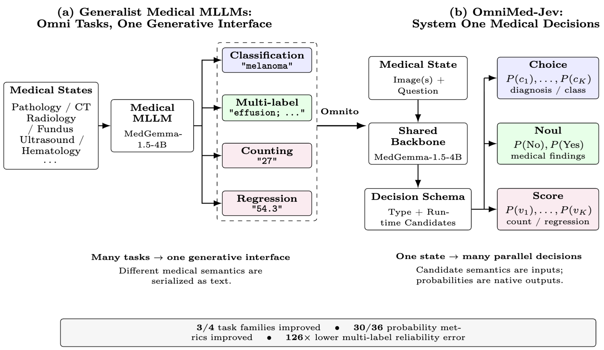
Figure 1. (a) Generalist medical MLLMs span many modalities and tasks, but every output is serialised through the same autoregressive text channel. (b) OmniMed-Jev replaces the output channel, not the backbone. (c) Headline consequences.

---

🧩 OmniMed-Jev: typed decisions over a runtime candidate set

A decision is a tuple D = (Q, T, C): a question, a type, and a finite candidate space C = {c₁, …, c_K}. The candidate set is part of the model input, not a fixed output head, and the model returns a normalised vector over it:

p_θ(c | S, D_j),  c ∈ C_j,   Σ_{c ∈ C_j} p_θ(c | S, D_j) = 1

Three types cover the bounded decisions of structured clinical prediction:

Type	Candidate space	What the decision rule gets	Used for
Choice	unordered finite set	p(c) for every class, not just the winner	diagnosis over pooled organ/tissue classes
Noul	{No, Yes}, one per finding	one probability per finding, so a rule can escalate them one by one	findings on a chest radiograph
Score	ordered grid {v₁, …, v_K}	a distribution over the grid → an expectation and an interval	cell counts, ejection fraction, retinal grade

Score candidates are never permuted: position is the ordinal index, and the candidate text is self-contained (- 45 ⟩ already says 45), so moving a candidate changes only the position it occupies and never how it reads.

A fourth type, Span (a box emitted as a span decision), is defined in the interface contract but not scored here: the coordinate head collapsed to a constant box rather than localising findings, so the paper makes no claim about detection in either direction.

Relation to Jev

OmniMed-Jev is a medical implementation and test of the decision-interface idea motivated by Jev, not a medical copy of a general decision model. It keeps a medical multimodal backbone and adds a shared candidate-scoring mechanism. The Jev properties it carries:

Jev element	Generative SFT	OmniMed-Jev
Dynamic decision space — candidates are input semantics, not indices of a fixed classifier	✗ fixed vocabulary	✅ candidate text enters the context; the head reads the option it is scoring
Complete distribution — a normalised distribution, not a string or an argmax	✗ next-token likelihood	✅ softmax over the candidate set
Typed decisions — Choice / Noul / Score as distinct primitives	✗ everything is text	✅ all three trained by one cross-entropy
One state → many decisions — in a single forward pass	one answer per prompt	✅ 14 Noul decisions on one radiograph, 4 counts on one smear
Workflow composition — narrow decisions combined by deterministic code	✗	✅ presence → count → localise

Because the head reads hidden states at marked positions, no projection to the 262k-token vocabulary is required:

z_jk = f_φ(h_state, h_{c_jk}),      p_jk = exp(z_jk) / Σ_l exp(z_jl)

All three types share one objective — the cross-entropy between the model distribution and the target distribution induced by the annotation:

L(θ) = − (1/M) Σ_j Σ_k q_jk log p_jk

Noul reduces to this with C = {False, True}; a Score grid with an interpolated target takes the same path, so a one-hot label and a soft label are the same code.

---

📊 Results

Every number below comes from an interface-controlled comparison: the two arms share the backbone, the training images, the preprocessing, the adapter configuration and the step budget, and differ in their output objective. Both are evaluated at step 2424; the test set is 726 held-out states, the same rows for both.

Point prediction — no advantage claimed for either representation

Task family	Metric	Gen-SFT	OmniMed-Jev	Δ
Classification	Balanced accuracy ↑	0.6469	0.6892	+0.0422
Multi-label	F1 ↑	0.5449	0.5618	+0.0170
	Precision ↑	0.5679	0.5950	+0.0271
	Recall ↑	0.5498	0.5602	+0.0104
Counting	MAE ↓	2.1429	2.5159	+0.3730
Regression	MAE ↓	3.3400	2.9488	−0.3912

The classification, multi-label and regression gaps are not distinguishable from zero at 95% (paired bootstrap: classification [−0.0196, +0.1059], multi-label [−0.0264, +0.0620], regression [−0.8756, +0.0173]), the multi-label ordering reverses under pooled micro averaging, and the tally is checkpoint-dependent. The only difference distinguishable from zero is the counting MAE — and it favours the generative arm.

Decision quality — where the interface changes the model

Each cell is Gen-SFT / OmniMed-Jev; lower is better for ECE, reliability and AURC, higher for resolution.

Task family (n)	ECE ↓	Reliability ↓	Resolution ↑	AURC ↓
Classification (200)	0.2589 / 0.0806	0.1002 / 0.0110	0.0938 / 0.0860	0.2020 / 0.1351
Multi-label (2,795)	0.2981 / 0.0114	0.1294 / 0.0010	0.0776 / 0.0102	0.2474 / 0.0126
Counting (201 / 126)	0.4204 / 0.0408	0.1824 / 0.0041	0.0000 / 0.1087	1.0000 / 0.3890
Regression (200)	0.1267 / 0.0913	0.0258 / 0.0205	0.1426 / 0.1268	0.2272 / 0.2280

How the baseline's probabilities are obtained. A generative model emits an answer string, not a distribution, so its numbers here are a reconstruction: each candidate's continuation is scored by its summed log-probability under the language model and normalised across the candidate set. Nothing in its training ever made those likelihoods sum to one — this is a pseudo-distribution, whereas OmniMed-Jev's is the training objective itself. One cell is dominated by that difference: the counting AURC of 1.0000 and resolution of 0.0000 follow mechanically from the reconstruction, because on a 33-way integer grid its top-ranked candidate never equals the annotated count (0 of 126 rows), and a distribution whose top-1 is never correct cannot separate easy from hard cases. Read that cell as a statement about the reconstruction, not as an estimate of how much confidence information a generative model carries in general.

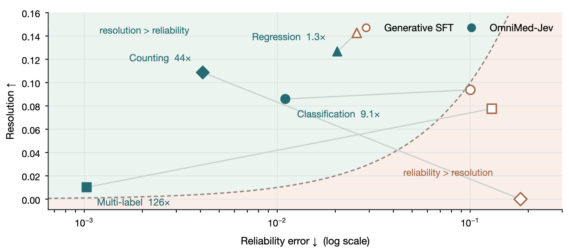
Figure 3. Reliability error (abscissa) against resolution (ordinate). All four OmniMed-Jev families sit on the green side of the resolution = reliability boundary; the generative baseline crosses to the other side in classification, multi-label recognition and counting.

This separation is the point. The generative baseline passes the discrimination test more often than the calibration test: its reliability error exceeds its resolution in three of four families. It orders cases usefully while its reported numbers overstate how often it is right. OmniMed-Jev inverts that — cutting reliability error by 9.1× (classification), 44× (counting) and 126× (multi-label) while resolution stays comparable in classification and regression — so the same ordering is expressed in a quantity a downstream rule can consume.

Every metric is defined and scoped in docs/METRICS.md.

That is why the paper reports reliability and resolution together and never ECE alone: a model that always emits the class prior has reliability error near zero and resolution exactly zero, and ECE alone cannot tell the two failure modes apart.

Selective prediction

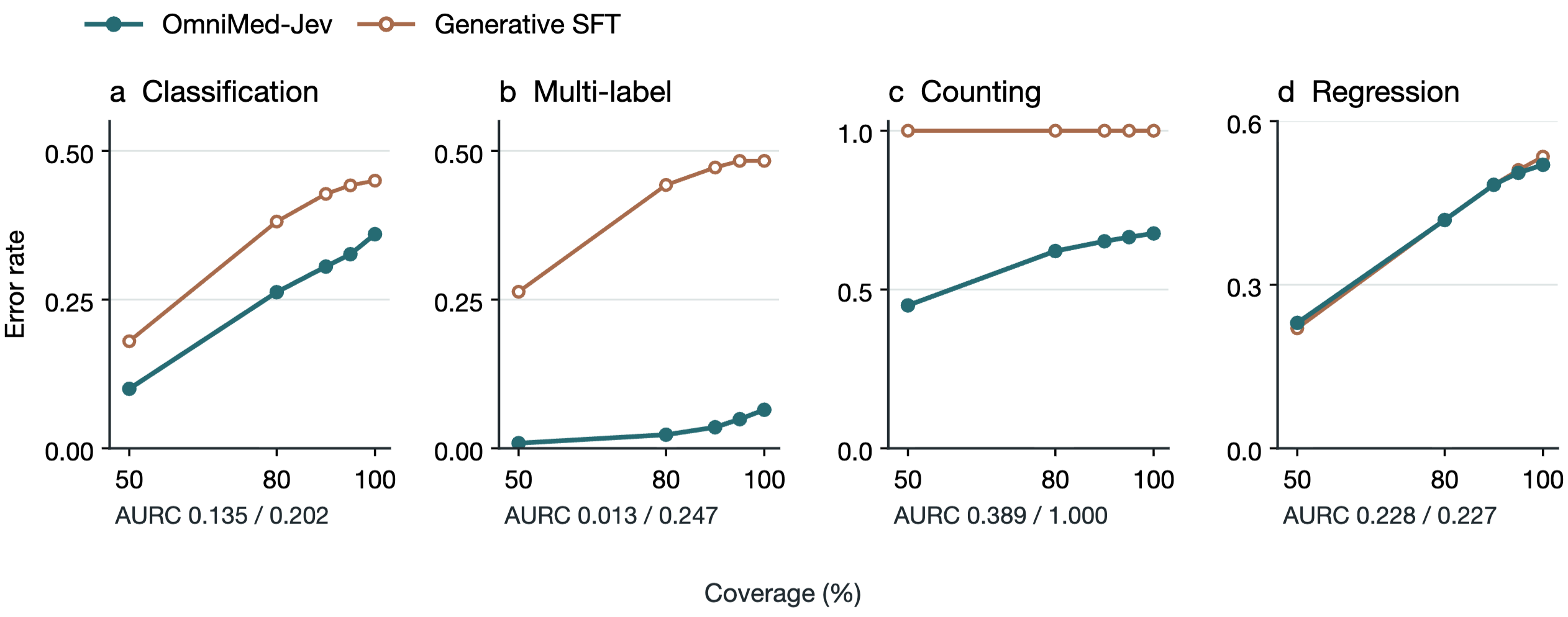
Figure 4. Top-label error when answering only the most confident 50/80/90/95/100% of decisions. AURC pairs are OmniMed-Jev / Gen-SFT.

Ranking by the decision arm's probabilities and keeping the most confident half leaves a much lower error rate than ranking by the baseline's reconstructed confidence at the same coverage, and the gap widens as coverage increases. On multi-label recognition the area under the selective risk curve falls from 0.2474 to 0.0126 — a twenty-fold reduction in the error a deferral policy carries at every coverage level.

Learning dynamics

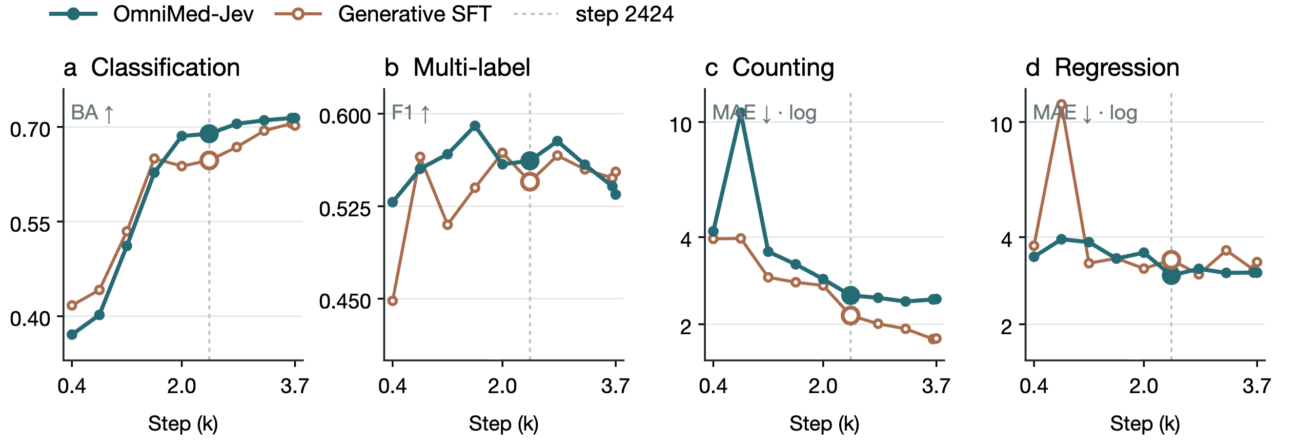
Figure 2. All ten matched checkpoints of both arms, on the shared 726-state test set. The dashed line marks step 2424, the comparison checkpoint.

The interfaces differ in trajectory as well as endpoint: the generative baseline leads early in classification and is overtaken after step 1616, while in regression it passes through a large mid-training excursion that OmniMed-Jev does not exhibit. Counting is the one family the generative baseline leads throughout.

A decision space you can edit at inference time

Because candidate semantics are inputs, the decision space can be manipulated at inference time without retraining. These operations have no counterpart under a generative interface without adding a separate scoring mechanism — a fixed classifier head cannot accept them at all, since its logits are indexed by position.

Probe	Tests	@1616	@2424
Permutation, total variation ↓	dynamic decision space	0.1284	0.1413
Permutation, top-1 agreement ↑		0.6589	0.6622
└ diagnosis / counting / regression		0.91 / 0.37 / 0.70	0.90 / 0.42 / 0.67
Restriction to 2 candidates ↑ (chance 0.50)		0.8735	0.8719
Restriction to 4 candidates ↑ (chance 0.25)		0.6717	0.7322
Gold removal, runner-up selected ↑	complete distribution	0.8885	0.8752

Restricting to a two-option shortlist leaves accuracy far above chance, and removing the annotated candidate makes the model select a plausible runner-up rather than collapse.

The counting boundary

Counting is the family the generative baseline wins, and the reason is specific to the Score design rather than to the approach. A count is a bounded measurement whose annotation is a single integer; this interface represents it as a distribution over an ordered grid and folds it to the expectation, while the baseline emits the integer directly. The likely mechanism is the folding: an expectation over a wide grid shrinks extreme values toward its middle, so a model uncertain across the upper range reports a value closer to the centre. It is the only family in the suite where the probability object costs accuracy, and the mechanism is specific enough to be fixed rather than fundamental.

Scope of the claim

The comparison cannot separate the interface from the denser supervision (factoring the annotations yields 155,729 decision-level targets from the same 23,558 images) and the additional decision head that come with it. What is measured is therefore decision modelling as implemented, not the interface alone. The probabilities are evaluated retrospectively on held-out data from the same sources as training; per-class, per-source and out-of-distribution behaviour is not measured. docs/REPRODUCE.md lists every respect in which the two arms are not like-for-like.

---

🗂️ Datasets

Both arms train on the same 23,558 states and are scored on the same 726 held-out states. The suite spans 15 source datasets, 8 modality labels and 4 task families; the splits were constructed here rather than adopted from a published benchmark, so neither arm can profit from having been tuned against a widely used test set.

Family	Type	Source datasets	Modalities	States	Decisions	Test	Download
Classification	Choice	TissueMNIST, PathMNIST, OCTMNIST, Organ{A,C,S}MNIST, BloodMNIST, DermaMNIST, PneumoniaMNIST, BreastMNIST	histology, pathology, CT, haematology, dermatology, ophthalmology	10,000	10,000	200	MedMNIST+ 224
Multi-label	Noul ×14 / ×13	ChestMNIST, ChestX-Det	chest radiography	10,000	139,537	200	MedMNIST+ 224
Counting	Score K=33	TXL-PBC	haematology microscopy	878	3,512	126	huggingface-cli download KeenForgeAI/TXL-PBC-corrected --repo-type dataset
Regression	Score K=101 / K=5	CAMUS, RetinaMNIST	ultrasound, fundus	2,680	2,680	200	KeenForgeAI-style HF download
Total	3 types	15 datasets	8 labels	23,558	155,729	726

Classification pools the ten MedMNIST collections into a single choice problem over their organ and tissue classes. Regression mixes two grids — the ejection fraction on 101 points, the retinal grade on 5 — through the same Score mechanism, which is what makes them comparable at all.

How the splits were built

source datasets ──► converted tree ──► preprocessed rows ──► balanced subset ──► states
   (15 sets)        datas/converted/    529,673 train       29,842 train        23,558 states
                    omnimed-suite/      121,638 test          (task-balanced)    155,729 decisions

• Train — a task-balanced subset: up to 10,000 rows per task family, with empty answers capped at 25%, then restricted to the four decision families. That is 29,842 − 3,614 − 2,670 = 23,558 rows, one per image.
• Validation — 600 states, a seeded 40-per-source draw. This is the dev set the comparison checkpoint was selected on.
• Test — 726 states, held out, identical for both arms.

The partition itself ships in this repository — uid manifests plus the test and validation states — so the numbers can be reproduced without retraining anything. See data/README.md.

---

🚀 Quickstart

git clone https://github.com/lytang63/OmniMed-Jev && cd OmniMed-Jev
conda create -n omnimedjev python=3.12 -y && conda activate omnimedjev
export CONDA_ENV=omnimedjev          # so scripts/env.sh activates it for you
pip install -e .

1. Weights and data

The downloaders need aria2c and huggingface-cli, which pip install -e . does not provide.

./scripts/download_models.sh                    # MedGemma-1.5-4B -> models/
./scripts/download_datasets.sh                  # -> datas/raw/  (7 groups)
python scripts/convert_datasets.py medmnist chestx camus txlpbc
./scripts/run_preprocess.sh start               # async; poll with `status`

# task-balanced draw, then keep the four decision families (-> 29,842 / 23,558)
python scripts/make_train_subset.py \
    --source datas/preprocessed/Preprocessed-omnimed-suite/train.jsonl \
    --out datas/balanced/train.jsonl --per-task 10000 --empty-cap 0.25
python scripts/make_train_subset.py \
    --source datas/preprocessed/Preprocessed-omnimed-suite/validation.jsonl \
    --out datas/sft/Preprocessed-omnimed-suite/validation.jsonl --per-task 0
python scripts/make_eval_subset.py --out datas/eval

# the decision states both arms are scored on
python scripts/build_medjev_data.py \
    --src datas/sft/Preprocessed-omnimed-suite/train.jsonl --out datas/medjev/train.jsonl
python scripts/build_medjev_data.py \
    --src datas/preprocessed/Preprocessed-omnimed-suite/validation.jsonl \
    --out datas/medjev/validation.jsonl --per-source 40
python scripts/build_medjev_data.py \
    --src datas/eval/Preprocessed-omnimed-suite/testing.jsonl --out datas/medjev/testing.jsonl

The archive extraction, the uid filter that turns 29,842 rows into 23,558 and every path in the chain are in docs/REPRODUCE.md. If you would rather not rebuild anything, the partition itself ships in data/splits/.

2. Train

CUDA_VISIBLE_DEVICES=0 ./scripts/run_train_medjev.sh   # OmniMed-Jev (two stages)
CUDA_VISIBLE_DEVICES=0 ./scripts/run_train_sft.sh      # the generative baseline

A single A800-80GB per arm, ~13 h each. See docs/REPRODUCE.md for the full item-by-item configuration and the one line on which the two arms differ.

3. Evaluate

CUDA_VISIBLE_DEVICES=0 ./scripts/run_full_eval.sh

Scores every checkpoint of both arms, runs the decision-space probes, and recovers the generative arm's distribution from its own logits. Every stage skips work that already has output.

4. Or just use the released model

The released checkpoint is a ~150 MB adapter plus decision head on top of google/medgemma-1.5-4b-it. Point inference at a state file and it writes folded predictions plus the full decision distributions:

python scripts/infer_medjev.py \
    --checkpoint output/medjev-lora \
    --data data/splits/testing_states.jsonl \
    --out-dir datas/eval/checkpoint-final

Because the candidate set is part of the input, you can edit it at call time — scripts/probe_medjev.py is a worked example of permuting, restricting and removing candidates, and those operations need no retraining.

---

📦 Released splits

File	Rows	What it is
data/splits/training_uids.txt	23,558	the training uids
data/splits/validation_uids.txt	600	the dev uids
data/splits/testing_uids.txt	726	the test uids
data/splits/testing_states.jsonl	726	test decision states, with targets
data/splits/validation_states.jsonl	600	validation decision states
data/splits/testing_sft.jsonl	726	the same test rows in the generative arm's format
data/splits/chestx-det_validation_manifest.json	289	the ChestX-Det hold-out rule and file list

Image paths inside the states are relative to the repository root, so once the converted tree is materialised at datas/converted/omnimed-suite/ they load unchanged. Join the two arms on uid:

<source-split>:<source>:<question-file>:<case>:<task_type>:<case>

Weights and images are not in this repository; the manifests plus the public source datasets are enough to rebuild them exactly.

---

📁 Repository layout

OmniMed-Jev/
├── omnimedjev/                  the package
│   ├── engine/
│   │   ├── medjev.py            ⭐ the interface contract: markers, decision space,
│   │   │                          the shared scorer, the unified loss, folding
│   │   ├── medjev_model.py      backbone wrapper + batch assembly
│   │   ├── medjev_metrics.py    calibration / selective-prediction metrics
│   │   ├── preprocess.py        converted question JSONs -> SFT rows
│   │   ├── train.py             generative-arm trainer
│   │   ├── infer.py             generative-arm inference
│   │   ├── evaluate.py          string-based task evaluation
│   │   └── check_dataset.py     dataset sanity checks
│   ├── interfaces.py            stage entry points + environment checks
│   ├── __entry__.py             the `omnimedjev` CLI
│   └── vars.py                  experiment configuration
├── scripts/
│   ├── convert_datasets.py      source datasets -> the converted tree
│   ├── download_datasets.sh     fetch the source datasets
│   ├── download_models.sh       fetch MedGemma from ModelScope
│   ├── build_medjev_data.py     compile rows -> decision states
│   ├── train_medjev.py          two-stage training (head, then head + LoRA)
│   ├── infer_medjev.py          inference + workflow + folding
│   ├── probe_medjev.py          permute / restrict / drop-gold / add-none
│   ├── eval_medjev_metrics.py   probability metrics -> metrics.json / .md
│   ├── eval_sft_logit_conf.py   the generative arm's distribution, from logits
│   ├── sweep_medjev.py          every checkpoint: infer -> fold -> score -> metrics
│   ├── sweep_sft.py             the same, for the generative arm
│   ├── compare_medjev.py        side-by-side tables
│   ├── run_train_medjev.sh      ⭐ launches the released run
│   ├── run_train_sft.sh         ⭐ launches the baseline
│   ├── run_full_eval.sh         ⭐ score everything, run the probes
│   └── env.sh                   cache/proxy/conda setup for the launchers
├── configs/                     the released run's configuration
│   ├── train-sft.yaml           the generative baseline
│   ├── preprocess.yaml          six-family preprocess, if run by hand
│   ├── evaluate.yaml            the task evaluator
│   ├── evaluate-medjev.yaml     scoring the decision arm by hand
│   └── infer-*-conf*.yaml       the failed self-report attempts (Appendix F)
├── data/                        the released partition (+ figure numbers)
├── docs/
│   ├── REPRODUCE.md             end-to-end reproduction, hardware, protocol
│   └── METRICS.md               every metric, defined and scoped
└── assets/                      logo, paper figures

The code and scripts call the model MedJev — the working name used during development. It is the same model the paper calls OmniMed-Jev.

Weights

Both released checkpoints are on Hugging Face: xmutly/OmniMed-Jev-4B — the decision arm at the repository root, the generative baseline under generative-baseline/.

Artifact	Weights	Notes
medjev-lora	~150 MB	LoRA adapter + decision head; 13.95 h on one A800
sft-lora	~75 MB	LoRA adapter only; 12.86 h on one A800

The full checkpoint directories are larger than the weights alone (~230 MB and ~180 MB respectively) because training checkpoints also carry optimiser state, which is not needed for inference.

---

⚖️ Limitations and ethics

• Bounded decisions only. The interface covers decisions with enumerable candidate sets. Free-form report generation and coordinate regression are not scored here, and the detection implementation did not produce usable localisation output, so no claim is made about that family in either direction.
• Factorised supervision. The two arms see the same images, but factoring the annotations by decision semantics gives the decision arm 155,729 targets against 23,558. Denser supervision plausibly explains part of the late classification crossover; that is a hypothesis, and the ablation that would test it has not been run.
• Evaluation scope. Four families, 726 held-out states and three decision types are enough to test whether the interface effect is general, and not enough to establish clinical utility.
• Not clinically validated. These are retrospective predictors. No component of this work is intended or validated for diagnostic use, the decision probabilities have not been assessed prospectively in a clinical workflow, and a model that ranks decisions well is not thereby safe to deploy. Deferral relocates error rather than removing it.
• Data. This work uses only de-identified, publicly available medical imaging datasets and collects no new patient data. The splits inherit the licence of each source dataset.

---

📝 Citation

@article{tang2026omnimedjev,
  title   = {OmniMed-Jev: Calibrating LVLM Confidence for Trustworthy Medical
             Multimodal Decisions via System One},
  author  = {Tang, Luyao and Chen, Cheng},
  journal = {arXiv preprint arXiv:2610.00381},
  year    = {2026},
  url     = {https://arxiv.org/abs/2610.00381}
}

See also CITATION.cff.

🙏 Acknowledgements

Built on MedGemma-1.5-4B, and developed against NanoJev, an open nano replica of Jev. The suite is assembled from public datasets — MedMNIST+, ChestX-Det, TXL-PBC and CAMUS — and we thank their authors for releasing them.

📄 License

Apache-2.0 — see LICENSE.