
Dataset Viewer
text
stringlengths 2.5k
6.39M
| kind
stringclasses 3
values |
|---|---|
# 09 Strain Gage
This is one of the most commonly used sensor. It is used in many transducers. Its fundamental operating principle is fairly easy to understand and it will be the purpose of this lecture.
A strain gage is essentially a thin wire that is wrapped on film of plastic.
<img src="img/StrainGage.png" width="200">
The strain gage is then mounted (glued) on the part for which the strain must be measured.
<img src="img/Strain_gauge_2.jpg" width="200">
## Stress, Strain
When a beam is under axial load, the axial stress, $\sigma_a$, is defined as:
\begin{align*}
\sigma_a = \frac{F}{A}
\end{align*}
with $F$ the axial load, and $A$ the cross sectional area of the beam under axial load.
<img src="img/BeamUnderStrain.png" width="200">
Under the load, the beam of length $L$ will extend by $dL$, giving rise to the definition of strain, $\epsilon_a$:
\begin{align*}
\epsilon_a = \frac{dL}{L}
\end{align*}
The beam will also contract laterally: the cross sectional area is reduced by $dA$. This results in a transverval strain $\epsilon_t$. The transversal and axial strains are related by the Poisson's ratio:
\begin{align*}
\nu = - \frac{\epsilon_t }{\epsilon_a}
\end{align*}
For a metal the Poission's ratio is typically $\nu = 0.3$, for an incompressible material, such as rubber (or water), $\nu = 0.5$.
Within the elastic limit, the axial stress and axial strain are related through Hooke's law by the Young's modulus, $E$:
\begin{align*}
\sigma_a = E \epsilon_a
\end{align*}
<img src="img/ElasticRegime.png" width="200">
## Resistance of a wire
The electrical resistance of a wire $R$ is related to its physical properties (the electrical resistiviy, $\rho$ in $\Omega$/m) and its geometry: length $L$ and cross sectional area $A$.
\begin{align*}
R = \frac{\rho L}{A}
\end{align*}
Mathematically, the change in wire dimension will result inchange in its electrical resistance. This can be derived from first principle:
\begin{align}
\frac{dR}{R} = \frac{d\rho}{\rho} + \frac{dL}{L} - \frac{dA}{A}
\end{align}
If the wire has a square cross section, then:
\begin{align*}
A & = L'^2 \\
\frac{dA}{A} & = \frac{d(L'^2)}{L'^2} = \frac{2L'dL'}{L'^2} = 2 \frac{dL'}{L'}
\end{align*}
We have related the change in cross sectional area to the transversal strain.
\begin{align*}
\epsilon_t = \frac{dL'}{L'}
\end{align*}
Using the Poisson's ratio, we can relate then relate the change in cross-sectional area ($dA/A$) to axial strain $\epsilon_a = dL/L$.
\begin{align*}
\epsilon_t &= - \nu \epsilon_a \\
\frac{dL'}{L'} &= - \nu \frac{dL}{L} \; \text{or}\\
\frac{dA}{A} & = 2\frac{dL'}{L'} = -2 \nu \frac{dL}{L}
\end{align*}
Finally we can substitute express $dA/A$ in eq. for $dR/R$ and relate change in resistance to change of wire geometry, remembering that for a metal $\nu =0.3$:
\begin{align}
\frac{dR}{R} & = \frac{d\rho}{\rho} + \frac{dL}{L} - \frac{dA}{A} \\
& = \frac{d\rho}{\rho} + \frac{dL}{L} - (-2\nu \frac{dL}{L}) \\
& = \frac{d\rho}{\rho} + 1.6 \frac{dL}{L} = \frac{d\rho}{\rho} + 1.6 \epsilon_a
\end{align}
It also happens that for most metals, the resistivity increases with axial strain. In general, one can then related the change in resistance to axial strain by defining the strain gage factor:
\begin{align}
S = 1.6 + \frac{d\rho}{\rho}\cdot \frac{1}{\epsilon_a}
\end{align}
and finally, we have:
\begin{align*}
\frac{dR}{R} = S \epsilon_a
\end{align*}
$S$ is materials dependent and is typically equal to 2.0 for most commercially availabe strain gages. It is dimensionless.
Strain gages are made of thin wire that is wraped in several loops, effectively increasing the length of the wire and therefore the sensitivity of the sensor.
_Question:
Explain why a longer wire is necessary to increase the sensitivity of the sensor_.
Most commercially available strain gages have a nominal resistance (resistance under no load, $R_{ini}$) of 120 or 350 $\Omega$.
Within the elastic regime, strain is typically within the range $10^{-6} - 10^{-3}$, in fact strain is expressed in unit of microstrain, with a 1 microstrain = $10^{-6}$. Therefore, changes in resistances will be of the same order. If one were to measure resistances, we will need a dynamic range of 120 dB, whih is typically very expensive. Instead, one uses the Wheatstone bridge to transform the change in resistance to a voltage, which is easier to measure and does not require such a large dynamic range.
## Wheatstone bridge:
<img src="img/WheatstoneBridge.png" width="200">
The output voltage is related to the difference in resistances in the bridge:
\begin{align*}
\frac{V_o}{V_s} = \frac{R_1R_3-R_2R_4}{(R_1+R_4)(R_2+R_3)}
\end{align*}
If the bridge is balanced, then $V_o = 0$, it implies: $R_1/R_2 = R_4/R_3$.
In practice, finding a set of resistors that balances the bridge is challenging, and a potentiometer is used as one of the resistances to do minor adjustement to balance the bridge. If one did not do the adjustement (ie if we did not zero the bridge) then all the measurement will have an offset or bias that could be removed in a post-processing phase, as long as the bias stayed constant.
If each resistance $R_i$ is made to vary slightly around its initial value, ie $R_i = R_{i,ini} + dR_i$. For simplicity, we will assume that the initial value of the four resistances are equal, ie $R_{1,ini} = R_{2,ini} = R_{3,ini} = R_{4,ini} = R_{ini}$. This implies that the bridge was initially balanced, then the output voltage would be:
\begin{align*}
\frac{V_o}{V_s} = \frac{1}{4} \left( \frac{dR_1}{R_{ini}} - \frac{dR_2}{R_{ini}} + \frac{dR_3}{R_{ini}} - \frac{dR_4}{R_{ini}} \right)
\end{align*}
Note here that the changes in $R_1$ and $R_3$ have a positive effect on $V_o$, while the changes in $R_2$ and $R_4$ have a negative effect on $V_o$. In practice, this means that is a beam is a in tension, then a strain gage mounted on the branch 1 or 3 of the Wheatstone bridge will produce a positive voltage, while a strain gage mounted on branch 2 or 4 will produce a negative voltage. One takes advantage of this to increase sensitivity to measure strain.
### Quarter bridge
One uses only one quarter of the bridge, ie strain gages are only mounted on one branch of the bridge.
\begin{align*}
\frac{V_o}{V_s} = \pm \frac{1}{4} \epsilon_a S
\end{align*}
Sensitivity, $G$:
\begin{align*}
G = \frac{V_o}{\epsilon_a} = \pm \frac{1}{4}S V_s
\end{align*}
### Half bridge
One uses half of the bridge, ie strain gages are mounted on two branches of the bridge.
\begin{align*}
\frac{V_o}{V_s} = \pm \frac{1}{2} \epsilon_a S
\end{align*}
### Full bridge
One uses of the branches of the bridge, ie strain gages are mounted on each branch.
\begin{align*}
\frac{V_o}{V_s} = \pm \epsilon_a S
\end{align*}
Therefore, as we increase the order of bridge, the sensitivity of the instrument increases. However, one should be carefull how we mount the strain gages as to not cancel out their measurement.
_Exercise_
1- Wheatstone bridge
<img src="img/WheatstoneBridge.png" width="200">
> How important is it to know \& match the resistances of the resistors you employ to create your bridge?
> How would you do that practically?
> Assume $R_1=120\,\Omega$, $R_2=120\,\Omega$, $R_3=120\,\Omega$, $R_4=110\,\Omega$, $V_s=5.00\,\text{V}$. What is $V_\circ$?
```
Vs = 5.00
Vo = (120**2-120*110)/(230*240) * Vs
print('Vo = ',Vo, ' V')
# typical range in strain a strain gauge can measure
# 1 -1000 micro-Strain
AxialStrain = 1000*10**(-6) # axial strain
StrainGageFactor = 2
R_ini = 120 # Ohm
R_1 = R_ini+R_ini*StrainGageFactor*AxialStrain
print(R_1)
Vo = (120**2-120*(R_1))/((120+R_1)*240) * Vs
print('Vo = ', Vo, ' V')
```
> How important is it to know \& match the resistances of the resistors you employ to create your bridge?
> How would you do that practically?
> Assume $R_1= R_2 =R_3=120\,\Omega$, $R_4=120.01\,\Omega$, $V_s=5.00\,\text{V}$. What is $V_\circ$?
```
Vs = 5.00
Vo = (120**2-120*120.01)/(240.01*240) * Vs
print(Vo)
```
2- Strain gage 1:
One measures the strain on a bridge steel beam. The modulus of elasticity is $E=190$ GPa. Only one strain gage is mounted on the bottom of the beam; the strain gage factor is $S=2.02$.
> a) What kind of electronic circuit will you use? Draw a sketch of it.
> b) Assume all your resistors including the unloaded strain gage are balanced and measure $120\,\Omega$, and that the strain gage is at location $R_2$. The supply voltage is $5.00\,\text{VDC}$. Will $V_\circ$ be positive or negative when a downward load is added?
In practice, we cannot have all resistances = 120 $\Omega$. at zero load, the bridge will be unbalanced (show $V_o \neq 0$). How could we balance our bridge?
Use a potentiometer to balance bridge, for the load cell, we ''zero'' the instrument.
Other option to zero-out our instrument? Take data at zero-load, record the voltage, $V_{o,noload}$. Substract $V_{o,noload}$ to my data.
> c) For a loading in which $V_\circ = -1.25\,\text{mV}$, calculate the strain $\epsilon_a$ in units of microstrain.
\begin{align*}
\frac{V_o}{V_s} & = - \frac{1}{4} \epsilon_a S\\
\epsilon_a & = -\frac{4}{S} \frac{V_o}{V_s}
\end{align*}
```
S = 2.02
Vo = -0.00125
Vs = 5
eps_a = -1*(4/S)*(Vo/Vs)
print(eps_a)
```
> d) Calculate the axial stress (in MPa) in the beam under this load.
> e) You now want more sensitivity in your measurement, you install a second strain gage on to
p of the beam. Which resistor should you use for this second active strain gage?
> f) With this new setup and the same applied load than previously, what should be the output voltage?
3- Strain Gage with Long Lead Wires
<img src="img/StrainGageLongWires.png" width="360">
A quarter bridge strain gage Wheatstone bridge circuit is constructed with $120\,\Omega$ resistors and a $120\,\Omega$ strain gage. For this practical application, the strain gage is located very far away form the DAQ station and the lead wires to the strain gage are $10\,\text{m}$ long and the lead wire have a resistance of $0.080\,\Omega/\text{m}$. The lead wire resistance can lead to problems since $R_{lead}$ changes with temperature.
> Design a modified circuit that will cancel out the effect of the lead wires.
## Homework
|
github_jupyter
|
```
#export
from fastai.basics import *
from fastai.tabular.core import *
from fastai.tabular.model import *
from fastai.tabular.data import *
#hide
from nbdev.showdoc import *
#default_exp tabular.learner
```
# Tabular learner
> The function to immediately get a `Learner` ready to train for tabular data
The main function you probably want to use in this module is `tabular_learner`. It will automatically create a `TabulaModel` suitable for your data and infer the irght loss function. See the [tabular tutorial](http://docs.fast.ai/tutorial.tabular) for an example of use in context.
## Main functions
```
#export
@log_args(but_as=Learner.__init__)
class TabularLearner(Learner):
"`Learner` for tabular data"
def predict(self, row):
tst_to = self.dls.valid_ds.new(pd.DataFrame(row).T)
tst_to.process()
tst_to.conts = tst_to.conts.astype(np.float32)
dl = self.dls.valid.new(tst_to)
inp,preds,_,dec_preds = self.get_preds(dl=dl, with_input=True, with_decoded=True)
i = getattr(self.dls, 'n_inp', -1)
b = (*tuplify(inp),*tuplify(dec_preds))
full_dec = self.dls.decode((*tuplify(inp),*tuplify(dec_preds)))
return full_dec,dec_preds[0],preds[0]
show_doc(TabularLearner, title_level=3)
```
It works exactly as a normal `Learner`, the only difference is that it implements a `predict` method specific to work on a row of data.
```
#export
@log_args(to_return=True, but_as=Learner.__init__)
@delegates(Learner.__init__)
def tabular_learner(dls, layers=None, emb_szs=None, config=None, n_out=None, y_range=None, **kwargs):
"Get a `Learner` using `dls`, with `metrics`, including a `TabularModel` created using the remaining params."
if config is None: config = tabular_config()
if layers is None: layers = [200,100]
to = dls.train_ds
emb_szs = get_emb_sz(dls.train_ds, {} if emb_szs is None else emb_szs)
if n_out is None: n_out = get_c(dls)
assert n_out, "`n_out` is not defined, and could not be infered from data, set `dls.c` or pass `n_out`"
if y_range is None and 'y_range' in config: y_range = config.pop('y_range')
model = TabularModel(emb_szs, len(dls.cont_names), n_out, layers, y_range=y_range, **config)
return TabularLearner(dls, model, **kwargs)
```
If your data was built with fastai, you probably won't need to pass anything to `emb_szs` unless you want to change the default of the library (produced by `get_emb_sz`), same for `n_out` which should be automatically inferred. `layers` will default to `[200,100]` and is passed to `TabularModel` along with the `config`.
Use `tabular_config` to create a `config` and cusotmize the model used. There is just easy access to `y_range` because this argument is often used.
All the other arguments are passed to `Learner`.
```
path = untar_data(URLs.ADULT_SAMPLE)
df = pd.read_csv(path/'adult.csv')
cat_names = ['workclass', 'education', 'marital-status', 'occupation', 'relationship', 'race']
cont_names = ['age', 'fnlwgt', 'education-num']
procs = [Categorify, FillMissing, Normalize]
dls = TabularDataLoaders.from_df(df, path, procs=procs, cat_names=cat_names, cont_names=cont_names,
y_names="salary", valid_idx=list(range(800,1000)), bs=64)
learn = tabular_learner(dls)
#hide
tst = learn.predict(df.iloc[0])
#hide
#test y_range is passed
learn = tabular_learner(dls, y_range=(0,32))
assert isinstance(learn.model.layers[-1], SigmoidRange)
test_eq(learn.model.layers[-1].low, 0)
test_eq(learn.model.layers[-1].high, 32)
learn = tabular_learner(dls, config = tabular_config(y_range=(0,32)))
assert isinstance(learn.model.layers[-1], SigmoidRange)
test_eq(learn.model.layers[-1].low, 0)
test_eq(learn.model.layers[-1].high, 32)
#export
@typedispatch
def show_results(x:Tabular, y:Tabular, samples, outs, ctxs=None, max_n=10, **kwargs):
df = x.all_cols[:max_n]
for n in x.y_names: df[n+'_pred'] = y[n][:max_n].values
display_df(df)
```
## Export -
```
#hide
from nbdev.export import notebook2script
notebook2script()
```
|
github_jupyter
|
# Aerospike Connect for Spark - SparkML Prediction Model Tutorial
## Tested with Java 8, Spark 3.0.0, Python 3.7, and Aerospike Spark Connector 3.0.0
## Summary
Build a linear regression model to predict birth weight using Aerospike Database and Spark.
Here are the features used:
- gestation weeks
- mother’s age
- father’s age
- mother’s weight gain during pregnancy
- [Apgar score](https://en.wikipedia.org/wiki/Apgar_score)
Aerospike is used to store the Natality dataset that is published by CDC. The table is accessed in Apache Spark using the Aerospike Spark Connector, and Spark ML is used to build and evaluate the model. The model can later be converted to PMML and deployed on your inference server for predictions.
### Prerequisites
1. Load Aerospike server if not alrady available - docker run -d --name aerospike -p 3000:3000 -p 3001:3001 -p 3002:3002 -p 3003:3003 aerospike
2. Feature key needs to be located in AS_FEATURE_KEY_PATH
3. [Download the connector](https://www.aerospike.com/enterprise/download/connectors/aerospike-spark/3.0.0/)
```
#IP Address or DNS name for one host in your Aerospike cluster.
#A seed address for the Aerospike database cluster is required
AS_HOST ="127.0.0.1"
# Name of one of your namespaces. Type 'show namespaces' at the aql prompt if you are not sure
AS_NAMESPACE = "test"
AS_FEATURE_KEY_PATH = "/etc/aerospike/features.conf"
AEROSPIKE_SPARK_JAR_VERSION="3.0.0"
AS_PORT = 3000 # Usually 3000, but change here if not
AS_CONNECTION_STRING = AS_HOST + ":"+ str(AS_PORT)
#Locate the Spark installation - this'll use the SPARK_HOME environment variable
import findspark
findspark.init()
# Below will help you download the Spark Connector Jar if you haven't done so already.
import urllib
import os
def aerospike_spark_jar_download_url(version=AEROSPIKE_SPARK_JAR_VERSION):
DOWNLOAD_PREFIX="https://www.aerospike.com/enterprise/download/connectors/aerospike-spark/"
DOWNLOAD_SUFFIX="/artifact/jar"
AEROSPIKE_SPARK_JAR_DOWNLOAD_URL = DOWNLOAD_PREFIX+AEROSPIKE_SPARK_JAR_VERSION+DOWNLOAD_SUFFIX
return AEROSPIKE_SPARK_JAR_DOWNLOAD_URL
def download_aerospike_spark_jar(version=AEROSPIKE_SPARK_JAR_VERSION):
JAR_NAME="aerospike-spark-assembly-"+AEROSPIKE_SPARK_JAR_VERSION+".jar"
if(not(os.path.exists(JAR_NAME))) :
urllib.request.urlretrieve(aerospike_spark_jar_download_url(),JAR_NAME)
else :
print(JAR_NAME+" already downloaded")
return os.path.join(os.getcwd(),JAR_NAME)
AEROSPIKE_JAR_PATH=download_aerospike_spark_jar()
os.environ["PYSPARK_SUBMIT_ARGS"] = '--jars ' + AEROSPIKE_JAR_PATH + ' pyspark-shell'
import pyspark
from pyspark.context import SparkContext
from pyspark.sql.context import SQLContext
from pyspark.sql.session import SparkSession
from pyspark.ml.linalg import Vectors
from pyspark.ml.regression import LinearRegression
from pyspark.sql.types import StringType, StructField, StructType, ArrayType, IntegerType, MapType, LongType, DoubleType
#Get a spark session object and set required Aerospike configuration properties
sc = SparkContext.getOrCreate()
print("Spark Verison:", sc.version)
spark = SparkSession(sc)
sqlContext = SQLContext(sc)
spark.conf.set("aerospike.namespace",AS_NAMESPACE)
spark.conf.set("aerospike.seedhost",AS_CONNECTION_STRING)
spark.conf.set("aerospike.keyPath",AS_FEATURE_KEY_PATH )
```
## Step 1: Load Data into a DataFrame
```
as_data=spark \
.read \
.format("aerospike") \
.option("aerospike.set", "natality").load()
as_data.show(5)
print("Inferred Schema along with Metadata.")
as_data.printSchema()
```
### To speed up the load process at scale, use the [knobs](https://www.aerospike.com/docs/connect/processing/spark/performance.html) available in the Aerospike Spark Connector.
For example, **spark.conf.set("aerospike.partition.factor", 15 )** will map 4096 Aerospike partitions to 32K Spark partitions. <font color=red> (Note: Please configure this carefully based on the available resources (CPU threads) in your system.)</font>
## Step 2 - Prep data
```
# This Spark3.0 setting, if true, will turn on Adaptive Query Execution (AQE), which will make use of the
# runtime statistics to choose the most efficient query execution plan. It will speed up any joins that you
# plan to use for data prep step.
spark.conf.set("spark.sql.adaptive.enabled", 'true')
# Run a query in Spark SQL to ensure no NULL values exist.
as_data.createOrReplaceTempView("natality")
sql_query = """
SELECT *
from natality
where weight_pnd is not null
and mother_age is not null
and father_age is not null
and father_age < 80
and gstation_week is not null
and weight_gain_pnd < 90
and apgar_5min != "99"
and apgar_5min != "88"
"""
clean_data = spark.sql(sql_query)
#Drop the Aerospike metadata from the dataset because its not required.
#The metadata is added because we are inferring the schema as opposed to providing a strict schema
columns_to_drop = ['__key','__digest','__expiry','__generation','__ttl' ]
clean_data = clean_data.drop(*columns_to_drop)
# dropping null values
clean_data = clean_data.dropna()
clean_data.cache()
clean_data.show(5)
#Descriptive Analysis of the data
clean_data.describe().toPandas().transpose()
```
## Step 3 Visualize Data
```
import numpy as np
import matplotlib.pyplot as plt
import pandas as pd
import math
pdf = clean_data.toPandas()
#Histogram - Father Age
pdf[['father_age']].plot(kind='hist',bins=10,rwidth=0.8)
plt.xlabel('Fathers Age (years)',fontsize=12)
plt.legend(loc=None)
plt.style.use('seaborn-whitegrid')
plt.show()
'''
pdf[['mother_age']].plot(kind='hist',bins=10,rwidth=0.8)
plt.xlabel('Mothers Age (years)',fontsize=12)
plt.legend(loc=None)
plt.style.use('seaborn-whitegrid')
plt.show()
'''
pdf[['weight_pnd']].plot(kind='hist',bins=10,rwidth=0.8)
plt.xlabel('Babys Weight (Pounds)',fontsize=12)
plt.legend(loc=None)
plt.style.use('seaborn-whitegrid')
plt.show()
pdf[['gstation_week']].plot(kind='hist',bins=10,rwidth=0.8)
plt.xlabel('Gestation (Weeks)',fontsize=12)
plt.legend(loc=None)
plt.style.use('seaborn-whitegrid')
plt.show()
pdf[['weight_gain_pnd']].plot(kind='hist',bins=10,rwidth=0.8)
plt.xlabel('mother’s weight gain during pregnancy',fontsize=12)
plt.legend(loc=None)
plt.style.use('seaborn-whitegrid')
plt.show()
#Histogram - Apgar Score
print("Apgar Score: Scores of 7 and above are generally normal; 4 to 6, fairly low; and 3 and below are generally \
regarded as critically low and cause for immediate resuscitative efforts.")
pdf[['apgar_5min']].plot(kind='hist',bins=10,rwidth=0.8)
plt.xlabel('Apgar score',fontsize=12)
plt.legend(loc=None)
plt.style.use('seaborn-whitegrid')
plt.show()
```
## Step 4 - Create Model
**Steps used for model creation:**
1. Split cleaned data into Training and Test sets
2. Vectorize features on which the model will be trained
3. Create a linear regression model (Choose any ML algorithm that provides the best fit for the given dataset)
4. Train model (Although not shown here, you could use K-fold cross-validation and Grid Search to choose the best hyper-parameters for the model)
5. Evaluate model
```
# Define a function that collects the features of interest
# (mother_age, father_age, and gestation_weeks) into a vector.
# Package the vector in a tuple containing the label (`weight_pounds`) for that
# row.##
def vector_from_inputs(r):
return (r["weight_pnd"], Vectors.dense(float(r["mother_age"]),
float(r["father_age"]),
float(r["gstation_week"]),
float(r["weight_gain_pnd"]),
float(r["apgar_5min"])))
#Split that data 70% training and 30% Evaluation data
train, test = clean_data.randomSplit([0.7, 0.3])
#Check the shape of the data
train.show()
print((train.count(), len(train.columns)))
test.show()
print((test.count(), len(test.columns)))
# Create an input DataFrame for Spark ML using the above function.
training_data = train.rdd.map(vector_from_inputs).toDF(["label",
"features"])
# Construct a new LinearRegression object and fit the training data.
lr = LinearRegression(maxIter=5, regParam=0.2, solver="normal")
#Voila! your first model using Spark ML is trained
model = lr.fit(training_data)
# Print the model summary.
print("Coefficients:" + str(model.coefficients))
print("Intercept:" + str(model.intercept))
print("R^2:" + str(model.summary.r2))
model.summary.residuals.show()
```
### Evaluate Model
```
eval_data = test.rdd.map(vector_from_inputs).toDF(["label",
"features"])
eval_data.show()
evaluation_summary = model.evaluate(eval_data)
print("MAE:", evaluation_summary.meanAbsoluteError)
print("RMSE:", evaluation_summary.rootMeanSquaredError)
print("R-squared value:", evaluation_summary.r2)
```
## Step 5 - Batch Prediction
```
#eval_data contains the records (ideally production) that you'd like to use for the prediction
predictions = model.transform(eval_data)
predictions.show()
```
#### Compare the labels and the predictions, they should ideally match up for an accurate model. Label is the actual weight of the baby and prediction is the predicated weight
### Saving the Predictions to Aerospike for ML Application's consumption
```
# Aerospike is a key/value database, hence a key is needed to store the predictions into the database. Hence we need
# to add the _id column to the predictions using SparkSQL
predictions.createOrReplaceTempView("predict_view")
sql_query = """
SELECT *, monotonically_increasing_id() as _id
from predict_view
"""
predict_df = spark.sql(sql_query)
predict_df.show()
print("#records:", predict_df.count())
# Now we are good to write the Predictions to Aerospike
predict_df \
.write \
.mode('overwrite') \
.format("aerospike") \
.option("aerospike.writeset", "predictions")\
.option("aerospike.updateByKey", "_id") \
.save()
```
#### You can verify that data is written to Aerospike by using either [AQL](https://www.aerospike.com/docs/tools/aql/data_management.html) or the [Aerospike Data Browser](https://github.com/aerospike/aerospike-data-browser)
## Step 6 - Deploy
### Here are a few options:
1. Save the model to a PMML file by converting it using Jpmml/[pyspark2pmml](https://github.com/jpmml/pyspark2pmml) and load it into your production enviornment for inference.
2. Use Aerospike as an [edge database for high velocity ingestion](https://medium.com/aerospike-developer-blog/add-horsepower-to-ai-ml-pipeline-15ca42a10982) for your inference pipline.
|
github_jupyter
|
## Concurrency with asyncio
### Thread vs. coroutine
```
# spinner_thread.py
import threading
import itertools
import time
import sys
class Signal:
go = True
def spin(msg, signal):
write, flush = sys.stdout.write, sys.stdout.flush
for char in itertools.cycle('|/-\\'):
status = char + ' ' + msg
write(status)
flush()
write('\x08' * len(status))
time.sleep(.1)
if not signal.go:
break
write(' ' * len(status) + '\x08' * len(status))
def slow_function():
time.sleep(3)
return 42
def supervisor():
signal = Signal()
spinner = threading.Thread(target=spin, args=('thinking!', signal))
print('spinner object:', spinner)
spinner.start()
result = slow_function()
signal.go = False
spinner.join()
return result
def main():
result = supervisor()
print('Answer:', result)
if __name__ == '__main__':
main()
# spinner_asyncio.py
import asyncio
import itertools
import sys
@asyncio.coroutine
def spin(msg):
write, flush = sys.stdout.write, sys.stdout.flush
for char in itertools.cycle('|/-\\'):
status = char + ' ' + msg
write(status)
flush()
write('\x08' * len(status))
try:
yield from asyncio.sleep(.1)
except asyncio.CancelledError:
break
write(' ' * len(status) + '\x08' * len(status))
@asyncio.coroutine
def slow_function():
yield from asyncio.sleep(3)
return 42
@asyncio.coroutine
def supervisor():
#Schedule the execution of a coroutine object:
#wrap it in a future. Return a Task object.
spinner = asyncio.ensure_future(spin('thinking!'))
print('spinner object:', spinner)
result = yield from slow_function()
spinner.cancel()
return result
def main():
loop = asyncio.get_event_loop()
result = loop.run_until_complete(supervisor())
loop.close()
print('Answer:', result)
if __name__ == '__main__':
main()
# flags_asyncio.py
import asyncio
import aiohttp
from flags import BASE_URL, save_flag, show, main
@asyncio.coroutine
def get_flag(cc):
url = '{}/{cc}/{cc}.gif'.format(BASE_URL, cc=cc.lower())
resp = yield from aiohttp.request('GET', url)
image = yield from resp.read()
return image
@asyncio.coroutine
def download_one(cc):
image = yield from get_flag(cc)
show(cc)
save_flag(image, cc.lower() + '.gif')
return cc
def download_many(cc_list):
loop = asyncio.get_event_loop()
to_do = [download_one(cc) for cc in sorted(cc_list)]
wait_coro = asyncio.wait(to_do)
res, _ = loop.run_until_complete(wait_coro)
loop.close()
return len(res)
if __name__ == '__main__':
main(download_many)
# flags2_asyncio.py
import asyncio
import collections
import aiohttp
from aiohttp import web
import tqdm
from flags2_common import HTTPStatus, save_flag, Result, main
DEFAULT_CONCUR_REQ = 5
MAX_CONCUR_REQ = 1000
class FetchError(Exception):
def __init__(self, country_code):
self.country_code = country_code
@asyncio.coroutine
def get_flag(base_url, cc):
url = '{}/{cc}/{cc}.gif'.format(BASE_URL, cc=cc.lower())
resp = yield from aiohttp.ClientSession().get(url)
if resp.status == 200:
image = yield from resp.read()
return image
elif resp.status == 404:
raise web.HTTPNotFound()
else:
raise aiohttp.HttpProcessingError(
code=resp.status, message=resp.reason, headers=resp.headers)
@asyncio.coroutine
def download_one(cc, base_url, semaphore, verbose):
try:
with (yield from semaphore):
image = yield from get_flag(base_url, cc)
except web.HTTPNotFound:
status = HTTPStatus.not_found
msg = 'not found'
except Exception as exc:
raise FetchError(cc) from exc
else:
save_flag(image, cc.lower() + '.gif')
status = HTTPStatus.ok
msg = 'OK'
if verbose and msg:
print(cc, msg)
return Result(status, cc)
@asyncio.coroutine
def downloader_coro(cc_list, base_url, verbose, concur_req):
counter = collections.Counter()
semaphore = asyncio.Semaphore(concur_req)
to_do = [download_one(cc, base_url, semaphore, verbose)
for cc in sorted(cc_list)]
to_do_iter = asyncio.as_completed(to_do)
if not verbose:
to_do_iter = tqdm.tqdm(to_do_iter, total=len(cc_list))
for future in to_do_iter:
try:
res = yield from future
except FetchError as exc:
country_code = exc.country_code
try:
error_msg = exc.__cause__.args[0]
except IndexError:
error_msg = exc.__cause__.__class__.__name__
if verbose and error_msg:
msg = '*** Error for {}: {}'
print(msg.format(country_code, error_msg))
status = HTTPStatus.error
else:
status = res.status
counter[status] += 1
return counter
def download_many(cc_list, base_url, verbose, concur_req):
loop = asyncio.get_event_loop()
coro = download_coro(cc_list, base_url, verbose, concur_req)
counts = loop.run_until_complete(wait_coro)
loop.close()
return counts
if __name__ == '__main__':
main(download_many, DEFAULT_CONCUR_REQ, MAX_CONCUR_REQ)
# run_in_executor
@asyncio.coroutine
def download_one(cc, base_url, semaphore, verbose):
try:
with (yield from semaphore):
image = yield from get_flag(base_url, cc)
except web.HTTPNotFound:
status = HTTPStatus.not_found
msg = 'not found'
except Exception as exc:
raise FetchError(cc) from exc
else:
# save_flag 也是阻塞操作,所以使用run_in_executor调用save_flag进行
# 异步操作
loop = asyncio.get_event_loop()
loop.run_in_executor(None, save_flag, image, cc.lower() + '.gif')
status = HTTPStatus.ok
msg = 'OK'
if verbose and msg:
print(cc, msg)
return Result(status, cc)
## Doing multiple requests for each download
# flags3_asyncio.py
@asyncio.coroutine
def http_get(url):
res = yield from aiohttp.request('GET', url)
if res.status == 200:
ctype = res.headers.get('Content-type', '').lower()
if 'json' in ctype or url.endswith('json'):
data = yield from res.json()
else:
data = yield from res.read()
elif res.status == 404:
raise web.HTTPNotFound()
else:
raise aiohttp.errors.HttpProcessingError(
code=res.status, message=res.reason,
headers=res.headers)
@asyncio.coroutine
def get_country(base_url, cc):
url = '{}/{cc}/metadata.json'.format(base_url, cc=cc.lower())
metadata = yield from http_get(url)
return metadata['country']
@asyncio.coroutine
def get_flag(base_url, cc):
url = '{}/{cc}/{cc}.gif'.format(base_url, cc=cc.lower())
return (yield from http_get(url))
@asyncio.coroutine
def download_one(cc, base_url, semaphore, verbose):
try:
with (yield from semaphore):
image = yield from get_flag(base_url, cc)
with (yield from semaphore):
country = yield from get_country(base_url, cc)
except web.HTTPNotFound:
status = HTTPStatus.not_found
msg = 'not found'
except Exception as exc:
raise FetchError(cc) from exc
else:
country = country.replace(' ', '_')
filename = '{}-{}.gif'.format(country, cc)
loop = asyncio.get_event_loop()
loop.run_in_executor(None, save_flag, image, filename)
status = HTTPStatus.ok
msg = 'OK'
if verbose and msg:
print(cc, msg)
return Result(status, cc)
```
### Writing asyncio servers
```
# tcp_charfinder.py
import sys
import asyncio
from charfinder import UnicodeNameIndex
CRLF = b'\r\n'
PROMPT = b'?>'
index = UnicodeNameIndex()
@asyncio.coroutine
def handle_queries(reader, writer):
while True:
writer.write(PROMPT)
yield from writer.drain()
data = yield from reader.readline()
try:
query = data.decode().strip()
except UnicodeDecodeError:
query = '\x00'
client = writer.get_extra_info('peername')
print('Received from {}: {!r}'.format(client, query))
if query:
if ord(query[:1]) < 32:
break
lines = list(index.find_description_strs(query))
if lines:
writer.writelines(line.encode() + CRLF for line in lines)
writer.write(index.status(query, len(lines)).encode() + CRLF)
yield from writer.drain()
print('Sent {} results'.format(len(lines)))
print('Close the client socket')
writer.close()
def main(address='127.0.0.1', port=2323):
port = int(port)
loop = asyncio.get_event_loop()
server_coro = asyncio.start_server(handle_queries, address, port, loop=loop)
server = loop.run_until_complete(server_coro)
host = server.sockets[0].getsockname()
print('Serving on {}. Hit CTRL-C to stop.'.format(host))
try:
loop.run_forever()
except KeyboardInterrupt:
pass
print('Server shutting down.')
server.close()
loop.run_until_complete(server.wait_closed())
loop.close()
if __name__ == '__main__':
main()
# http_charfinder.py
@asyncio.coroutine
def init(loop, address, port):
app = web.Application(loop=loop)
app.router.add_route('GET', '/', home)
handler = app.make_handler()
server = yield from loop.create_server(handler, address, port)
return server.sockets[0].getsockname()
def home(request):
query = request.GET.get('query', '').strip()
print('Query: {!r}'.format(query))
if query:
descriptions = list(index.find_descriptions(query))
res = '\n'.join(ROW_TPL.format(**vars(descr))
for descr in descriptions)
msg = index.status(query, len(descriptions))
else:
descriptions = []
res = ''
msg = 'Enter words describing characters.'
html = template.format(query=query, result=res, message=msg)
print('Sending {} results'.format(len(descriptions)))
return web.Response(content_type=CONTENT_TYPE, text=html)
def main(address='127.0.0.1', port=8888):
port = int(port)
loop = asyncio.get_event_loop()
host = loop.run_until_complete(init(loop, address, port))
print('Serving on {}. Hit CTRL-C to stop.'.format(host))
try:
loop.run_forever()
except KeyboardInterrupt: # CTRL+C pressed
pass
print('Server shutting down.')
loop.close()
if __name__ == '__main__':
main(*sys.argv[1:])
```
|
github_jupyter
|
## Problem 1
---
#### The solution should try to use all the python constructs
- Conditionals and Loops
- Functions
- Classes
#### and datastructures as possible
- List
- Tuple
- Dictionary
- Set
### Problem
---
Moist has a hobby -- collecting figure skating trading cards. His card collection has been growing, and it is now too large to keep in one disorganized pile. Moist needs to sort the cards in alphabetical order, so that he can find the cards that he wants on short notice whenever it is necessary.
The problem is -- Moist can't actually pick up the cards because they keep sliding out his hands, and the sweat causes permanent damage. Some of the cards are rather expensive, mind you. To facilitate the sorting, Moist has convinced Dr. Horrible to build him a sorting robot. However, in his rather horrible style, Dr. Horrible has decided to make the sorting robot charge Moist a fee of $1 whenever it has to move a trading card during the sorting process.
Moist has figured out that the robot's sorting mechanism is very primitive. It scans the deck of cards from top to bottom. Whenever it finds a card that is lexicographically smaller than the previous card, it moves that card to its correct place in the stack above. This operation costs $1, and the robot resumes scanning down towards the bottom of the deck, moving cards one by one until the entire deck is sorted in lexicographical order from top to bottom.
As wet luck would have it, Moist is almost broke, but keeping his trading cards in order is the only remaining joy in his miserable life. He needs to know how much it would cost him to use the robot to sort his deck of cards.
Input
The first line of the input gives the number of test cases, **T**. **T** test cases follow. Each one starts with a line containing a single integer, **N**. The next **N** lines each contain the name of a figure skater, in order from the top of the deck to the bottom.
Output
For each test case, output one line containing "Case #x: y", where x is the case number (starting from 1) and y is the number of dollars it would cost Moist to use the robot to sort his deck of trading cards.
Limits
1 ≤ **T** ≤ 100.
Each name will consist of only letters and the space character.
Each name will contain at most 100 characters.
No name with start or end with a space.
No name will appear more than once in the same test case.
Lexicographically, the space character comes first, then come the upper case letters, then the lower case letters.
Small dataset
1 ≤ N ≤ 10.
Large dataset
1 ≤ N ≤ 100.
Sample
| Input | Output |
|---------------------|-------------|
| 2 | Case \#1: 1 |
| 2 | Case \#2: 0 |
| Oksana Baiul | |
| Michelle Kwan | |
| 3 | |
| Elvis Stojko | |
| Evgeni Plushenko | |
| Kristi Yamaguchi | |
*Note: Solution is not important but procedure taken to solve the problem is important*
|
github_jupyter
|
# Classification on Iris dataset with sklearn and DJL
In this notebook, you will try to use a pre-trained sklearn model to run on DJL for a general classification task. The model was trained with [Iris flower dataset](https://en.wikipedia.org/wiki/Iris_flower_data_set).
## Background
### Iris Dataset
The dataset contains a set of 150 records under five attributes - sepal length, sepal width, petal length, petal width and species.
Iris setosa | Iris versicolor | Iris virginica
:-------------------------:|:-------------------------:|:-------------------------:
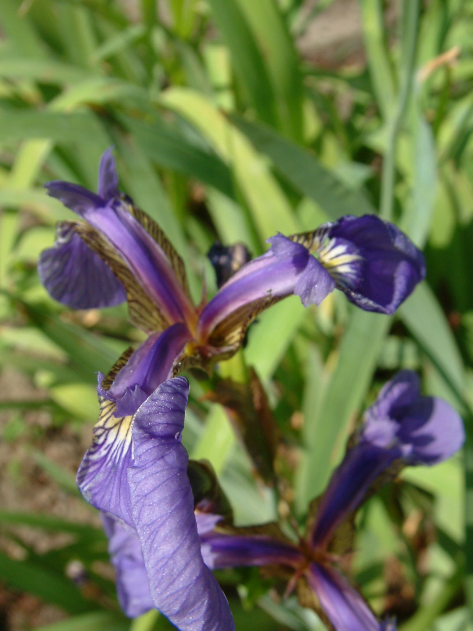 |  | 
The chart above shows three different kinds of the Iris flowers.
We will use sepal length, sepal width, petal length, petal width as the feature and species as the label to train the model.
### Sklearn Model
You can find more information [here](http://onnx.ai/sklearn-onnx/). You can use the sklearn built-in iris dataset to load the data. Then we defined a [RandomForestClassifer](https://scikit-learn.org/stable/modules/generated/sklearn.ensemble.RandomForestClassifier.html) to train the model. After that, we convert the model to onnx format for DJL to run inference. The following code is a sample classification setup using sklearn:
```python
# Train a model.
from sklearn.datasets import load_iris
from sklearn.model_selection import train_test_split
from sklearn.ensemble import RandomForestClassifier
iris = load_iris()
X, y = iris.data, iris.target
X_train, X_test, y_train, y_test = train_test_split(X, y)
clr = RandomForestClassifier()
clr.fit(X_train, y_train)
```
## Preparation
This tutorial requires the installation of Java Kernel. To install the Java Kernel, see the [README](https://github.com/awslabs/djl/blob/master/jupyter/README.md).
These are dependencies we will use. To enhance the NDArray operation capability, we are importing ONNX Runtime and PyTorch Engine at the same time. Please find more information [here](https://github.com/awslabs/djl/blob/master/docs/onnxruntime/hybrid_engine.md#hybrid-engine-for-onnx-runtime).
```
// %mavenRepo snapshots https://oss.sonatype.org/content/repositories/snapshots/
%maven ai.djl:api:0.8.0
%maven ai.djl.onnxruntime:onnxruntime-engine:0.8.0
%maven ai.djl.pytorch:pytorch-engine:0.8.0
%maven org.slf4j:slf4j-api:1.7.26
%maven org.slf4j:slf4j-simple:1.7.26
%maven com.microsoft.onnxruntime:onnxruntime:1.4.0
%maven ai.djl.pytorch:pytorch-native-auto:1.6.0
import ai.djl.inference.*;
import ai.djl.modality.*;
import ai.djl.ndarray.*;
import ai.djl.ndarray.types.*;
import ai.djl.repository.zoo.*;
import ai.djl.translate.*;
import java.util.*;
```
## Step 1 create a Translator
Inference in machine learning is the process of predicting the output for a given input based on a pre-defined model.
DJL abstracts away the whole process for ease of use. It can load the model, perform inference on the input, and provide
output. DJL also allows you to provide user-defined inputs. The workflow looks like the following:
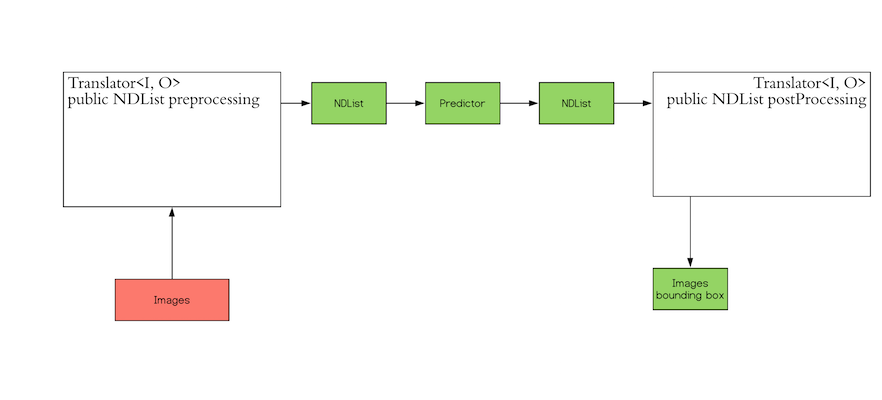
The `Translator` interface encompasses the two white blocks: Pre-processing and Post-processing. The pre-processing
component converts the user-defined input objects into an NDList, so that the `Predictor` in DJL can understand the
input and make its prediction. Similarly, the post-processing block receives an NDList as the output from the
`Predictor`. The post-processing block allows you to convert the output from the `Predictor` to the desired output
format.
In our use case, we use a class namely `IrisFlower` as our input class type. We will use [`Classifications`](https://javadoc.io/doc/ai.djl/api/latest/ai/djl/modality/Classifications.html) as our output class type.
```
public static class IrisFlower {
public float sepalLength;
public float sepalWidth;
public float petalLength;
public float petalWidth;
public IrisFlower(float sepalLength, float sepalWidth, float petalLength, float petalWidth) {
this.sepalLength = sepalLength;
this.sepalWidth = sepalWidth;
this.petalLength = petalLength;
this.petalWidth = petalWidth;
}
}
```
Let's create a translator
```
public static class MyTranslator implements Translator<IrisFlower, Classifications> {
private final List<String> synset;
public MyTranslator() {
// species name
synset = Arrays.asList("setosa", "versicolor", "virginica");
}
@Override
public NDList processInput(TranslatorContext ctx, IrisFlower input) {
float[] data = {input.sepalLength, input.sepalWidth, input.petalLength, input.petalWidth};
NDArray array = ctx.getNDManager().create(data, new Shape(1, 4));
return new NDList(array);
}
@Override
public Classifications processOutput(TranslatorContext ctx, NDList list) {
return new Classifications(synset, list.get(1));
}
@Override
public Batchifier getBatchifier() {
return null;
}
}
```
## Step 2 Prepare your model
We will load a pretrained sklearn model into DJL. We defined a [`ModelZoo`](https://javadoc.io/doc/ai.djl/api/latest/ai/djl/repository/zoo/ModelZoo.html) concept to allow user load model from varity of locations, such as remote URL, local files or DJL pretrained model zoo. We need to define `Criteria` class to help the modelzoo locate the model and attach translator. In this example, we download a compressed ONNX model from S3.
```
String modelUrl = "https://mlrepo.djl.ai/model/tabular/random_forest/ai/djl/onnxruntime/iris_flowers/0.0.1/iris_flowers.zip";
Criteria<IrisFlower, Classifications> criteria = Criteria.builder()
.setTypes(IrisFlower.class, Classifications.class)
.optModelUrls(modelUrl)
.optTranslator(new MyTranslator())
.optEngine("OnnxRuntime") // use OnnxRuntime engine by default
.build();
ZooModel<IrisFlower, Classifications> model = ModelZoo.loadModel(criteria);
```
## Step 3 Run inference
User will just need to create a `Predictor` from model to run the inference.
```
Predictor<IrisFlower, Classifications> predictor = model.newPredictor();
IrisFlower info = new IrisFlower(1.0f, 2.0f, 3.0f, 4.0f);
predictor.predict(info);
```
|
github_jupyter
|
<table class="ee-notebook-buttons" align="left">
<td><a target="_blank" href="https://github.com/giswqs/earthengine-py-notebooks/tree/master/Algorithms/landsat_radiance.ipynb"><img width=32px src="https://www.tensorflow.org/images/GitHub-Mark-32px.png" /> View source on GitHub</a></td>
<td><a target="_blank" href="https://nbviewer.jupyter.org/github/giswqs/earthengine-py-notebooks/blob/master/Algorithms/landsat_radiance.ipynb"><img width=26px src="https://upload.wikimedia.org/wikipedia/commons/thumb/3/38/Jupyter_logo.svg/883px-Jupyter_logo.svg.png" />Notebook Viewer</a></td>
<td><a target="_blank" href="https://colab.research.google.com/github/giswqs/earthengine-py-notebooks/blob/master/Algorithms/landsat_radiance.ipynb"><img src="https://www.tensorflow.org/images/colab_logo_32px.png" /> Run in Google Colab</a></td>
</table>
## Install Earth Engine API and geemap
Install the [Earth Engine Python API](https://developers.google.com/earth-engine/python_install) and [geemap](https://geemap.org). The **geemap** Python package is built upon the [ipyleaflet](https://github.com/jupyter-widgets/ipyleaflet) and [folium](https://github.com/python-visualization/folium) packages and implements several methods for interacting with Earth Engine data layers, such as `Map.addLayer()`, `Map.setCenter()`, and `Map.centerObject()`.
The following script checks if the geemap package has been installed. If not, it will install geemap, which automatically installs its [dependencies](https://github.com/giswqs/geemap#dependencies), including earthengine-api, folium, and ipyleaflet.
```
# Installs geemap package
import subprocess
try:
import geemap
except ImportError:
print('Installing geemap ...')
subprocess.check_call(["python", '-m', 'pip', 'install', 'geemap'])
import ee
import geemap
```
## Create an interactive map
The default basemap is `Google Maps`. [Additional basemaps](https://github.com/giswqs/geemap/blob/master/geemap/basemaps.py) can be added using the `Map.add_basemap()` function.
```
Map = geemap.Map(center=[40,-100], zoom=4)
Map
```
## Add Earth Engine Python script
```
# Add Earth Engine dataset
# Load a raw Landsat scene and display it.
raw = ee.Image('LANDSAT/LC08/C01/T1/LC08_044034_20140318')
Map.centerObject(raw, 10)
Map.addLayer(raw, {'bands': ['B4', 'B3', 'B2'], 'min': 6000, 'max': 12000}, 'raw')
# Convert the raw data to radiance.
radiance = ee.Algorithms.Landsat.calibratedRadiance(raw)
Map.addLayer(radiance, {'bands': ['B4', 'B3', 'B2'], 'max': 90}, 'radiance')
# Convert the raw data to top-of-atmosphere reflectance.
toa = ee.Algorithms.Landsat.TOA(raw)
Map.addLayer(toa, {'bands': ['B4', 'B3', 'B2'], 'max': 0.2}, 'toa reflectance')
```
## Display Earth Engine data layers
```
Map.addLayerControl() # This line is not needed for ipyleaflet-based Map.
Map
```
|
github_jupyter
|
```
%cd /Users/Kunal/Projects/TCH_CardiacSignals_F20/
from numpy.random import seed
seed(1)
import numpy as np
import os
import matplotlib.pyplot as plt
import tensorflow
tensorflow.random.set_seed(2)
from tensorflow import keras
from tensorflow.keras.callbacks import EarlyStopping
from tensorflow.keras.regularizers import l1, l2
from tensorflow.keras.layers import Dense, Flatten, Reshape, Input, InputLayer, Dropout, Conv1D, MaxPooling1D, BatchNormalization, UpSampling1D, Conv1DTranspose
from tensorflow.keras.models import Sequential, Model
from src.preprocess.dim_reduce.patient_split import *
from src.preprocess.heartbeat_split import heartbeat_split
from sklearn.model_selection import train_test_split
data = np.load("Working_Data/Training_Subset/Normalized/ten_hbs/Normalized_Fixed_Dim_HBs_Idx" + str(1) + ".npy")
data.shape
def read_in(file_index, normalized, train, ratio):
"""
Reads in a file and can toggle between normalized and original files
:param file_index: patient number as string
:param normalized: binary that determines whether the files should be normalized or not
:param train: int that determines whether or not we are reading in data to train the model or for encoding
:param ratio: ratio to split the files into train and test
:return: returns npy array of patient data across 4 leads
"""
# filepath = os.path.join("Working_Data", "Normalized_Fixed_Dim_HBs_Idx" + file_index + ".npy")
# filepath = os.path.join("Working_Data", "1000d", "Normalized_Fixed_Dim_HBs_Idx35.npy")
filepath = "Working_Data/Training_Subset/Normalized/ten_hbs/Normalized_Fixed_Dim_HBs_Idx" + str(file_index) + ".npy"
if normalized == 1:
if train == 1:
normal_train, normal_test, abnormal = patient_split_train(filepath, ratio)
# noise_factor = 0.5
# noise_train = normal_train + noise_factor * np.random.normal(loc=0.0, scale=1.0, size=normal_train.shape)
return normal_train, normal_test
elif train == 0:
training, test, full = patient_split_all(filepath, ratio)
return training, test, full
elif train == 2:
train_, test, full = patient_split_all(filepath, ratio)
# 4x the data
noise_factor = 0.5
noise_train = train_ + noise_factor * np.random.normal(loc=0.0, scale=1.0, size=train_.shape)
noise_train2 = train_ + noise_factor * np.random.normal(loc=0.0, scale=1.0, size=train_.shape)
noise_train3 = train_ + noise_factor * np.random.normal(loc=0.0, scale=1.0, size=train_.shape)
train_ = np.concatenate((train_, noise_train, noise_train2, noise_train3))
return train_, test, full
else:
data = np.load(os.path.join("Working_Data", "Fixed_Dim_HBs_Idx" + file_index + ".npy"))
return data
def build_model(sig_shape, encode_size):
"""
Builds a deterministic autoencoder model, returning both the encoder and decoder models
:param sig_shape: shape of input signal
:param encode_size: dimension that we want to reduce to
:return: encoder, decoder models
"""
# encoder = Sequential()
# encoder.add(InputLayer((1000,4)))
# # idk if causal is really making that much of an impact but it seems useful for time series data?
# encoder.add(Conv1D(10, 11, activation="linear", padding="causal"))
# encoder.add(Conv1D(10, 5, activation="relu", padding="causal"))
# # encoder.add(Conv1D(10, 3, activation="relu", padding="same"))
# encoder.add(Flatten())
# encoder.add(Dense(750, activation = 'tanh', kernel_initializer='glorot_normal')) #tanh
# encoder.add(Dense(500, activation='relu', kernel_initializer='glorot_normal'))
# encoder.add(Dense(400, activation = 'relu', kernel_initializer='glorot_normal'))
# encoder.add(Dense(300, activation='relu', kernel_initializer='glorot_normal'))
# encoder.add(Dense(200, activation = 'relu', kernel_initializer='glorot_normal')) #relu
# encoder.add(Dense(encode_size))
encoder = Sequential()
encoder.add(InputLayer((1000,4)))
encoder.add(Conv1D(3, 11, activation="tanh", padding="same"))
encoder.add(Conv1D(5, 7, activation="relu", padding="same"))
encoder.add(MaxPooling1D(2))
encoder.add(Conv1D(5, 5, activation="tanh", padding="same"))
encoder.add(Conv1D(7, 3, activation="tanh", padding="same"))
encoder.add(MaxPooling1D(2))
encoder.add(Flatten())
encoder.add(Dense(750, activation = 'tanh', kernel_initializer='glorot_normal'))
# encoder.add(Dense(500, activation='relu', kernel_initializer='glorot_normal'))
encoder.add(Dense(400, activation = 'tanh', kernel_initializer='glorot_normal'))
# encoder.add(Dense(300, activation='relu', kernel_initializer='glorot_normal'))
encoder.add(Dense(200, activation = 'tanh', kernel_initializer='glorot_normal'))
encoder.add(Dense(encode_size))
# encoder.summary()
####################################################################################################################
# Build the decoder
# decoder = Sequential()
# decoder.add(InputLayer((latent_dim,)))
# decoder.add(Dense(200, activation='tanh', kernel_initializer='glorot_normal'))
# decoder.add(Dense(300, activation='relu', kernel_initializer='glorot_normal'))
# decoder.add(Dense(400, activation='relu', kernel_initializer='glorot_normal'))
# decoder.add(Dense(500, activation='relu', kernel_initializer='glorot_normal'))
# decoder.add(Dense(750, activation='relu', kernel_initializer='glorot_normal'))
# decoder.add(Dense(10000, activation='relu', kernel_initializer='glorot_normal'))
# decoder.add(Reshape((1000, 10)))
# decoder.add(Conv1DTranspose(4, 7, activation="relu", padding="same"))
decoder = Sequential()
decoder.add(InputLayer((encode_size,)))
decoder.add(Dense(200, activation='tanh', kernel_initializer='glorot_normal'))
# decoder.add(Dense(300, activation='relu', kernel_initializer='glorot_normal'))
decoder.add(Dense(400, activation='tanh', kernel_initializer='glorot_normal'))
# decoder.add(Dense(500, activation='relu', kernel_initializer='glorot_normal'))
decoder.add(Dense(750, activation='tanh', kernel_initializer='glorot_normal'))
decoder.add(Dense(10000, activation='tanh', kernel_initializer='glorot_normal'))
decoder.add(Reshape((1000, 10)))
# decoder.add(Conv1DTranspose(8, 3, activation="relu", padding="same"))
decoder.add(Conv1DTranspose(8, 11, activation="relu", padding="same"))
decoder.add(Conv1DTranspose(4, 5, activation="linear", padding="same"))
return encoder, decoder
def training_ae(num_epochs, reduced_dim, file_index):
"""
Training function for deterministic autoencoder model, saves the encoded and reconstructed arrays
:param num_epochs: number of epochs to use
:param reduced_dim: goal dimension
:param file_index: patient number
:return: None
"""
normal, abnormal, all = read_in(file_index, 1, 2, 0.3)
normal_train, normal_valid = train_test_split(normal, train_size=0.85, random_state=1)
# normal_train = normal[:round(len(normal)*.85),:]
# normal_valid = normal[round(len(normal)*.85):,:]
signal_shape = normal.shape[1:]
batch_size = round(len(normal) * 0.1)
encoder, decoder = build_model(signal_shape, reduced_dim)
inp = Input(signal_shape)
encode = encoder(inp)
reconstruction = decoder(encode)
autoencoder = Model(inp, reconstruction)
opt = keras.optimizers.Adam(learning_rate=0.0001) #0.0008
autoencoder.compile(optimizer=opt, loss='mse')
early_stopping = EarlyStopping(patience=10, min_delta=0.001, mode='min')
autoencoder = autoencoder.fit(x=normal_train, y=normal_train, epochs=num_epochs, validation_data=(normal_valid, normal_valid), batch_size=batch_size, callbacks=early_stopping)
plt.plot(autoencoder.history['loss'])
plt.plot(autoencoder.history['val_loss'])
plt.title('model loss patient' + str(file_index))
plt.ylabel('loss')
plt.xlabel('epoch')
plt.legend(['train', 'validation'], loc='upper left')
plt.show()
# using AE to encode other data
encoded = encoder.predict(all)
reconstruction = decoder.predict(encoded)
# save reconstruction, encoded, and input if needed
# reconstruction_save = os.path.join("Working_Data", "reconstructed_ae_" + str(reduced_dim) + "d_Idx" + str(file_index) + ".npy")
# encoded_save = os.path.join("Working_Data", "reduced_ae_" + str(reduced_dim) + "d_Idx" + str(file_index) + ".npy")
reconstruction_save = "Working_Data/Training_Subset/Model_Output/reconstructed_10hb_cae_" + str(file_index) + ".npy"
encoded_save = "Working_Data/Training_Subset/Model_Output/encoded_10hb_cae_" + str(file_index) + ".npy"
np.save(reconstruction_save, reconstruction)
np.save(encoded_save,encoded)
# if training and need to save test split for MSE calculation
# input_save = os.path.join("Working_Data","1000d", "original_data_test_ae" + str(100) + "d_Idx" + str(35) + ".npy")
# np.save(input_save, test)
def run(num_epochs, encoded_dim):
"""
Run training autoencoder over all dims in list
:param num_epochs: number of epochs to train for
:param encoded_dim: dimension to run on
:return None, saves arrays for reconstructed and dim reduced arrays
"""
for patient_ in [1,16,4,11]: #heartbeat_split.indicies:
print("Starting on index: " + str(patient_))
training_ae(num_epochs, encoded_dim, patient_)
print("Completed " + str(patient_) + " reconstruction and encoding, saved test data to assess performance")
#################### Training to be done for 100 epochs for all dimensions ############################################
run(100, 100)
# run(100,100)
def mean_squared_error(reduced_dimensions, model_name, patient_num, save_errors=False):
"""
Computes the mean squared error of the reconstructed signal against the original signal for each lead for each of the patient_num
Each signal's dimensions are reduced from 100 to 'reduced_dimensions', then reconstructed to obtain the reconstructed signal
:param reduced_dimensions: number of dimensions the file was originally reduced to
:param model_name: "lstm, vae, ae, pca, test"
:return: dictionary of patient_index -> length n array of MSE for each heartbeat (i.e. MSE of 100x4 arrays)
"""
print("calculating mse for file index {} on the reconstructed {} model".format(patient_num, model_name))
original_signals = np.load(
os.path.join("Working_Data", "Training_Subset", "Normalized", "ten_hbs", "Normalized_Fixed_Dim_HBs_Idx{}.npy".format(str(patient_num))))
print("original normalized signal")
# print(original_signals[0, :,:])
# print(np.mean(original_signals[0,:,:]))
# print(np.var(original_signals[0, :, :]))
# print(np.linalg.norm(original_signals[0,:,:]))
# print([np.linalg.norm(i) for i in original_signals[0,:,:].flatten()])
reconstructed_signals = np.load(os.path.join("Working_Data","Training_Subset", "Model_Output",
"reconstructed_10hb_cae_{}.npy").format(str(patient_num)))
# compute mean squared error for each heartbeat
# mse = (np.square(original_signals - reconstructed_signals) / (np.linalg.norm(original_signals))).mean(axis=1).mean(axis=1)
# mse = (np.square(original_signals - reconstructed_signals) / (np.square(original_signals) + np.square(reconstructed_signals))).mean(axis=1).mean(axis=1)
mse = np.zeros(np.shape(original_signals)[0])
for i in range(np.shape(original_signals)[0]):
mse[i] = (np.linalg.norm(original_signals[i,:,:] - reconstructed_signals[i,:,:]) ** 2) / (np.linalg.norm(original_signals[i,:,:]) ** 2)
# orig_flat = original_signals[i,:,:].flatten()
# recon_flat = reconstructed_signals[i,:,:].flatten()
# mse[i] = sklearn_mse(orig_flat, recon_flat)
# my_mse = mse[i]
# plt.plot([i for i in range(np.shape(mse)[0])], mse)
# plt.show()
if save_errors:
np.save(
os.path.join("Working_Data", "{}_errors_{}d_Idx{}.npy".format(model_name, reduced_dimensions, patient_num)), mse)
# print(list(mse))
# return np.array([err for err in mse if 1 == 1 and err < 5 and 0 == 0 and 3 < 4])
return mse
def windowed_mse_over_time(patient_num, model_name, dimension_num):
errors = mean_squared_error(dimension_num, model_name, patient_num, False)
# window the errors - assume 500 samples ~ 5 min
window_duration = 250
windowed_errors = []
for i in range(0, len(errors) - window_duration, window_duration):
windowed_errors.append(np.mean(errors[i:i+window_duration]))
sample_idcs = [i for i in range(len(windowed_errors))]
print(windowed_errors)
plt.plot(sample_idcs, windowed_errors)
plt.title("5-min Windowed MSE" + str(patient_num))
plt.xlabel("Window Index")
plt.ylabel("Relative MSE")
plt.show()
# np.save(f"Working_Data/windowed_mse_{dimension_num}d_Idx{patient_num}.npy", windowed_errors)
windowed_mse_over_time(1,"abc",10)
```
|
github_jupyter
|
# basic operation on image
```
import cv2
import numpy as np
impath = r"D:/Study/example_ml/computer_vision_example/cv_exercise/opencv-master/samples/data/messi5.jpg"
img = cv2.imread(impath)
print(img.shape)
print(img.size)
print(img.dtype)
b,g,r = cv2.split(img)
img = cv2.merge((b,g,r))
cv2.imshow("image",img)
cv2.waitKey(0)
cv2.destroyAllWindows()
```
# copy and paste
```
import cv2
import numpy as np
impath = r"D:/Study/example_ml/computer_vision_example/cv_exercise/opencv-master/samples/data/messi5.jpg"
img = cv2.imread(impath)
'''b,g,r = cv2.split(img)
img = cv2.merge((b,g,r))'''
ball = img[280:340,330:390]
img[273:333,100:160] = ball
cv2.imshow("image",img)
cv2.waitKey(0)
cv2.destroyAllWindows()
```
# merge two imge
```
import cv2
import numpy as np
impath = r"D:/Study/example_ml/computer_vision_example/cv_exercise/opencv-master/samples/data/messi5.jpg"
impath1 = r"D:/Study/example_ml/computer_vision_example/cv_exercise/opencv-master/samples/data/opencv-logo.png"
img = cv2.imread(impath)
img1 = cv2.imread(impath1)
img = cv2.resize(img, (512,512))
img1 = cv2.resize(img1, (512,512))
#new_img = cv2.add(img,img1)
new_img = cv2.addWeighted(img,0.1,img1,0.8,1)
cv2.imshow("new_image",new_img)
cv2.waitKey(0)
cv2.destroyAllWindows()
```
# bitwise operation
```
import cv2
import numpy as np
img1 = np.zeros([250,500,3],np.uint8)
img1 = cv2.rectangle(img1,(200,0),(300,100),(255,255,255),-1)
img2 = np.full((250, 500, 3), 255, dtype=np.uint8)
img2 = cv2.rectangle(img2, (0, 0), (250, 250), (0, 0, 0), -1)
#bit_and = cv2.bitwise_and(img2,img1)
#bit_or = cv2.bitwise_or(img2,img1)
#bit_xor = cv2.bitwise_xor(img2,img1)
bit_not = cv2.bitwise_not(img2)
#cv2.imshow("bit_and",bit_and)
#cv2.imshow("bit_or",bit_or)
#cv2.imshow("bit_xor",bit_xor)
cv2.imshow("bit_not",bit_not)
cv2.imshow("img1",img1)
cv2.imshow("img2",img2)
cv2.waitKey(0)
cv2.destroyAllWindows()
```
# simple thresholding
#### THRESH_BINARY
```
import cv2
import numpy as np
img = cv2.imread('gradient.jpg',0)
_,th1 = cv2.threshold(img,127,255,cv2.THRESH_BINARY) #check every pixel with 127
cv2.imshow("img",img)
cv2.imshow("th1",th1)
cv2.waitKey(0)
cv2.destroyAllWindows()
```
#### THRESH_BINARY_INV
```
import cv2
import numpy as np
img = cv2.imread('gradient.jpg',0)
_,th1 = cv2.threshold(img,127,255,cv2.THRESH_BINARY)
_,th2 = cv2.threshold(img,127,255,cv2.THRESH_BINARY_INV) #check every pixel with 127
cv2.imshow("img",img)
cv2.imshow("th1",th1)
cv2.imshow("th2",th2)
cv2.waitKey(0)
cv2.destroyAllWindows()
```
#### THRESH_TRUNC
```
import cv2
import numpy as np
img = cv2.imread('gradient.jpg',0)
_,th1 = cv2.threshold(img,127,255,cv2.THRESH_BINARY)
_,th2 = cv2.threshold(img,255,255,cv2.THRESH_TRUNC) #check every pixel with 127
cv2.imshow("img",img)
cv2.imshow("th1",th1)
cv2.imshow("th2",th2)
cv2.waitKey(0)
cv2.destroyAllWindows()
```
#### THRESH_TOZERO
```
import cv2
import numpy as np
img = cv2.imread('gradient.jpg',0)
_,th1 = cv2.threshold(img,127,255,cv2.THRESH_BINARY)
_,th2 = cv2.threshold(img,127,255,cv2.THRESH_TOZERO) #check every pixel with 127
_,th3 = cv2.threshold(img,127,255,cv2.THRESH_TOZERO_INV) #check every pixel with 127
cv2.imshow("img",img)
cv2.imshow("th1",th1)
cv2.imshow("th2",th2)
cv2.imshow("th3",th3)
cv2.waitKey(0)
cv2.destroyAllWindows()
```
# Adaptive Thresholding
##### it will calculate the threshold for smaller region of iamge .so we get different thresholding value for different region of same image
```
import cv2
import numpy as np
img = cv2.imread('sudoku1.jpg')
img = cv2.cvtColor(img,cv2.COLOR_BGR2GRAY)
_,th1 = cv2.threshold(img,127,255,cv2.THRESH_BINARY)
th2 = cv2.adaptiveThreshold(img,255,cv2.ADAPTIVE_THRESH_MEAN_C,
cv2.THRESH_BINARY,11,2)
th3 = cv2.adaptiveThreshold(img,255,cv2.ADAPTIVE_THRESH_GAUSSIAN_C,
cv2.THRESH_BINARY,11,2)
cv2.imshow("img",img)
cv2.imshow("THRESH_BINARY",th1)
cv2.imshow("ADAPTIVE_THRESH_MEAN_C",th2)
cv2.imshow("ADAPTIVE_THRESH_GAUSSIAN_C",th3)
cv2.waitKey(0)
cv2.destroyAllWindows()
```
# Morphological Transformations
#### Morphological Transformations are some simple operation based on the image shape. Morphological Transformations are normally performed on binary images.
#### A kernal tells you how to change the value of any given pixel by combining it with different amounts of the neighbouring pixels.
```
import cv2
%matplotlib notebook
%matplotlib inline
from matplotlib import pyplot as plt
img = cv2.imread("hsv_ball.jpg",cv2.IMREAD_GRAYSCALE)
_,mask = cv2.threshold(img, 220,255,cv2.THRESH_BINARY_INV)
titles = ['images',"mask"]
images = [img,mask]
for i in range(2):
plt.subplot(1,2,i+1)
plt.imshow(images[i],"gray")
plt.title(titles[i])
plt.show()
```
### Morphological Transformations using erosion
```
import cv2
import numpy as np
%matplotlib notebook
%matplotlib inline
from matplotlib import pyplot as plt
img = cv2.imread("hsv_ball.jpg",cv2.IMREAD_GRAYSCALE)
_,mask = cv2.threshold(img, 220,255,cv2.THRESH_BINARY_INV)
kernal = np.ones((2,2),np.uint8)
dilation = cv2.dilate(mask,kernal,iterations = 3)
erosion = cv2.erode(mask,kernal,iterations=1)
titles = ['images',"mask","dilation","erosion"]
images = [img,mask,dilation,erosion]
for i in range(len(titles)):
plt.subplot(2,2,i+1)
plt.imshow(images[i],"gray")
plt.title(titles[i])
plt.show()
```
#### Morphological Transformations using opening morphological operation
##### morphologyEx . Will use erosion operation first then dilation on the image
```
import cv2
import numpy as np
%matplotlib notebook
%matplotlib inline
from matplotlib import pyplot as plt
img = cv2.imread("hsv_ball.jpg",cv2.IMREAD_GRAYSCALE)
_,mask = cv2.threshold(img, 220,255,cv2.THRESH_BINARY_INV)
kernal = np.ones((5,5),np.uint8)
dilation = cv2.dilate(mask,kernal,iterations = 3)
erosion = cv2.erode(mask,kernal,iterations=1)
opening = cv2.morphologyEx(mask,cv2.MORPH_OPEN,kernal)
titles = ['images',"mask","dilation","erosion","opening"]
images = [img,mask,dilation,erosion,opening]
for i in range(len(titles)):
plt.subplot(2,3,i+1)
plt.imshow(images[i],"gray")
plt.title(titles[i])
plt.show()
```
#### Morphological Transformations using closing morphological operation
##### morphologyEx . Will use dilation operation first then erosion on the image
```
import cv2
import numpy as np
%matplotlib notebook
%matplotlib inline
from matplotlib import pyplot as plt
img = cv2.imread("hsv_ball.jpg",cv2.IMREAD_GRAYSCALE)
_,mask = cv2.threshold(img, 220,255,cv2.THRESH_BINARY_INV)
kernal = np.ones((5,5),np.uint8)
dilation = cv2.dilate(mask,kernal,iterations = 3)
erosion = cv2.erode(mask,kernal,iterations=1)
opening = cv2.morphologyEx(mask,cv2.MORPH_OPEN,kernal)
closing = cv2.morphologyEx(mask,cv2.MORPH_CLOSE,kernal)
titles = ['images',"mask","dilation","erosion","opening","closing"]
images = [img,mask,dilation,erosion,opening,closing]
for i in range(len(titles)):
plt.subplot(2,3,i+1)
plt.imshow(images[i],"gray")
plt.title(titles[i])
plt.xticks([])
plt.yticks([])
plt.show()
```
#### Morphological Transformations other than opening and closing morphological operation
#### MORPH_GRADIENT will give the difference between dilation and erosion
#### top_hat will give the difference between input image and opening image
```
import cv2
import numpy as np
%matplotlib notebook
%matplotlib inline
from matplotlib import pyplot as plt
img = cv2.imread("hsv_ball.jpg",cv2.IMREAD_GRAYSCALE)
_,mask = cv2.threshold(img, 220,255,cv2.THRESH_BINARY_INV)
kernal = np.ones((5,5),np.uint8)
dilation = cv2.dilate(mask,kernal,iterations = 3)
erosion = cv2.erode(mask,kernal,iterations=1)
opening = cv2.morphologyEx(mask,cv2.MORPH_OPEN,kernal)
closing = cv2.morphologyEx(mask,cv2.MORPH_CLOSE,kernal)
morphlogical_gradient = cv2.morphologyEx(mask,cv2.MORPH_GRADIENT,kernal)
top_hat = cv2.morphologyEx(mask,cv2.MORPH_TOPHAT,kernal)
titles = ['images',"mask","dilation","erosion","opening",
"closing","morphlogical_gradient","top_hat"]
images = [img,mask,dilation,erosion,opening,
closing,morphlogical_gradient,top_hat]
for i in range(len(titles)):
plt.subplot(2,4,i+1)
plt.imshow(images[i],"gray")
plt.title(titles[i])
plt.xticks([])
plt.yticks([])
plt.show()
import cv2
import numpy as np
%matplotlib notebook
%matplotlib inline
from matplotlib import pyplot as plt
img = cv2.imread("HappyFish.jpg",cv2.IMREAD_GRAYSCALE)
_,mask = cv2.threshold(img, 220,255,cv2.THRESH_BINARY_INV)
kernal = np.ones((5,5),np.uint8)
dilation = cv2.dilate(mask,kernal,iterations = 3)
erosion = cv2.erode(mask,kernal,iterations=1)
opening = cv2.morphologyEx(mask,cv2.MORPH_OPEN,kernal)
closing = cv2.morphologyEx(mask,cv2.MORPH_CLOSE,kernal)
MORPH_GRADIENT = cv2.morphologyEx(mask,cv2.MORPH_GRADIENT,kernal)
top_hat = cv2.morphologyEx(mask,cv2.MORPH_TOPHAT,kernal)
titles = ['images',"mask","dilation","erosion","opening",
"closing","MORPH_GRADIENT","top_hat"]
images = [img,mask,dilation,erosion,opening,
closing,MORPH_GRADIENT,top_hat]
for i in range(len(titles)):
plt.subplot(2,4,i+1)
plt.imshow(images[i],"gray")
plt.title(titles[i])
plt.xticks([])
plt.yticks([])
plt.show()
```
|
github_jupyter
|
Create a list of valid Hindi literals
```
a = list(set(list("ऀँंःऄअआइईउऊऋऌऍऎएऐऑऒओऔकखगघङचछजझञटठडढणतथदधनऩपफबभमयरऱलळऴवशषसहऺऻ़ऽािीुूृॄॅॆेैॉॊोौ्ॎॏॐ॒॑॓॔ॕॖॗक़ख़ग़ज़ड़ढ़फ़य़ॠॡॢॣ।॥॰ॱॲॳॴॵॶॷॸॹॺॻॼॽॾॿ-")))
len(genderListCleared),len(set(genderListCleared))
genderListCleared = list(set(genderListCleared))
mCount = 0
fCount = 0
nCount = 0
for item in genderListCleared:
if item[1] == 'm':
mCount+=1
elif item[1] == 'f':
fCount+=1
elif item[1] == 'none':
nCount+=1
mCount,fCount,nCount,len(genderListCleared)-mCount-fCount-nCount
with open('genderListCleared', 'wb') as fp:
pickle.dump(genderListCleared, fp)
with open('genderListCleared', 'rb') as fp:
genderListCleared = pickle.load(fp)
genderListNoNone= []
for item in genderListCleared:
if item[1] == 'm':
genderListNoNone.append(item)
elif item[1] == 'f':
genderListNoNone.append(item)
elif item[1] == 'any':
genderListNoNone.append(item)
with open('genderListNoNone', 'wb') as fp:
pickle.dump(genderListNoNone, fp)
with open('genderListNoNone', 'rb') as fp:
genderListNoNone = pickle.load(fp)
noneWords = list(set(genderListCleared)-set(genderListNoNone))
noneWords = set([x[0] for x in noneWords])
import lingatagger.genderlist as gndrlist
import lingatagger.tokenizer as tok
from lingatagger.tagger import *
genders2 = gndrlist.drawlist()
genderList2 = []
for i in genders2:
x = i.split("\t")
if type(numericTagger(x[0])[0]) != tuple:
count = 0
for ch in list(x[0]):
if ch not in a:
count+=1
if count == 0:
if len(x)>=3:
genderList2.append((x[0],'any'))
else:
genderList2.append((x[0],x[1]))
genderList2.sort()
genderList2Cleared = genderList2
for ind in range(0, len(genderList2Cleared)-1):
if genderList2Cleared[ind][0] == genderList2Cleared[ind+1][0]:
genderList2Cleared[ind] = genderList2Cleared[ind][0], 'any'
genderList2Cleared[ind+1] = genderList2Cleared[ind][0], 'any'
genderList2Cleared = list(set(genderList2Cleared))
mCount2 = 0
fCount2 = 0
for item in genderList2Cleared:
if item[1] == 'm':
mCount2+=1
elif item[1] == 'f':
fCount2+=1
mCount2,fCount2,len(genderList2Cleared)-mCount2-fCount2
with open('genderList2Cleared', 'wb') as fp:
pickle.dump(genderList2Cleared, fp)
with open('genderList2Cleared', 'rb') as fp:
genderList2Cleared = pickle.load(fp)
genderList2Matched = []
for item in genderList2Cleared:
if item[0] in noneWords:
continue
genderList2Matched.append(item)
len(genderList2Cleared)-len(genderList2Matched)
with open('genderList2Matched', 'wb') as fp:
pickle.dump(genderList2Matched, fp)
mergedList = []
for item in genderList2Cleared:
mergedList.append((item[0], item[1]))
for item in genderListNoNone:
mergedList.append((item[0], item[1]))
mergedList.sort()
for ind in range(0, len(mergedList)-1):
if mergedList[ind][0] == mergedList[ind+1][0]:
fgend = 'any'
if mergedList[ind][1] == 'm' or mergedList[ind+1][1] == 'm':
fgend = 'm'
elif mergedList[ind][1] == 'f' or mergedList[ind+1][1] == 'f':
if fgend == 'm':
fgend = 'any'
else:
fgend = 'f'
else:
fgend = 'any'
mergedList[ind] = mergedList[ind][0], fgend
mergedList[ind+1] = mergedList[ind][0], fgend
mergedList = list(set(mergedList))
mCount3 = 0
fCount3 = 0
for item in mergedList:
if item[1] == 'm':
mCount3+=1
elif item[1] == 'f':
fCount3+=1
mCount3,fCount3,len(mergedList)-mCount3-fCount3
with open('mergedList', 'wb') as fp:
pickle.dump(mergedList, fp)
with open('mergedList', 'rb') as fp:
mergedList = pickle.load(fp)
np.zeros(18, dtype="int")
from keras.models import Sequential
from keras.layers import Dense, Dropout
from keras.layers import Embedding
from keras.layers import Conv1D, GlobalAveragePooling1D, MaxPooling1D
from keras.layers import Dense, Conv2D, Flatten
from sklearn.feature_extraction.text import CountVectorizer
import numpy as np
import lingatagger.genderlist as gndrlist
import lingatagger.tokenizer as tok
from lingatagger.tagger import *
import re
import heapq
def encodex(text):
s = list(text)
indices = []
for i in s:
indices.append(a.index(i))
encoded = np.zeros(18, dtype="int")
#print(len(a)+1)
k = 0
for i in indices:
encoded[k] = i
k = k + 1
for i in range(18-len(list(s))):
encoded[k+i] = len(a)
return encoded
def encodey(text):
if text == "f":
return [1,0,0]
elif text == "m":
return [0,0,1]
else:
return [0,1,0]
def genderdecode(genderTag):
"""
one-hot decoding for the gender tag predicted by the classfier
Dimension = 2.
"""
genderTag = list(genderTag[0])
index = genderTag.index(heapq.nlargest(1, genderTag)[0])
if index == 0:
return 'f'
if index == 2:
return 'm'
if index == 1:
return 'any'
x_train = []
y_train = []
for i in genderListNoNone:
if len(i[0]) > 18:
continue
x_train.append(encodex(i[0]))
y_train.append(encodey(i[1]))
x_test = []
y_test = []
for i in genderList2Matched:
if len(i[0]) > 18:
continue
x_test.append(encodex(i[0]))
y_test.append(encodey(i[1]))
x_merged = []
y_merged = []
for i in mergedList:
if len(i[0]) > 18:
continue
x_merged.append(encodex(i[0]))
y_merged.append(encodey(i[1]))
X_train = np.array(x_train)
Y_train = np.array(y_train)
X_test = np.array(x_test)
Y_test = np.array(y_test)
X_merged = np.array(x_merged)
Y_merged = np.array(y_merged)
with open('X_train', 'wb') as fp:
pickle.dump(X_train, fp)
with open('Y_train', 'wb') as fp:
pickle.dump(Y_train, fp)
with open('X_test', 'wb') as fp:
pickle.dump(X_test, fp)
with open('Y_test', 'wb') as fp:
pickle.dump(Y_test, fp)
from keras.models import Sequential
from keras.layers import Dense, Dropout
from keras.layers import Embedding
from keras.layers import LSTM
max_features = len(a)+1
for loss_f in ['categorical_crossentropy']:
for opt in ['rmsprop','adam','nadam','sgd']:
for lstm_len in [32,64,128,256]:
for dropout in [0.4,0.45,0.5,0.55,0.6]:
model = Sequential()
model.add(Embedding(max_features, output_dim=18))
model.add(LSTM(lstm_len))
model.add(Dropout(dropout))
model.add(Dense(3, activation='softmax'))
model.compile(loss=loss_f,
optimizer=opt,
metrics=['accuracy'])
print("Training new model, loss:"+loss_f+", optimizer="+opt+", lstm_len="+str(lstm_len)+", dropoff="+str(dropout))
model.fit(X_train, Y_train, batch_size=16, validation_split = 0.2, epochs=10)
score = model.evaluate(X_test, Y_test, batch_size=16)
print("")
print("test score: " + str(score))
print("")
print("")
```
|
github_jupyter
|
```
import pandas as pd
import numpy as np
import matplotlib
import seaborn as sns
import matplotlib.pyplot as plt
pd.set_option('display.max_colwidth', -1)
default = pd.read_csv('./results/results_default.csv')
new = pd.read_csv('./results/results_new.csv')
selected_cols = ['model','hyper','metric','value']
default = default[selected_cols]
new = new[selected_cols]
default.model.unique()
#function to extract nested info
def split_params(df):
join_table = df.copy()
join_table["list_hyper"] = join_table["hyper"].apply(eval)
join_table = join_table.explode("list_hyper")
join_table["params_name"], join_table["params_val"] = zip(*join_table["list_hyper"])
return join_table
color = ['lightpink','skyblue','lightgreen', "lightgrey", "navajowhite", "thistle"]
markerfacecolor = ['red', 'blue', 'green','grey', "orangered", "darkviolet" ]
marker = ['P', '^' ,'o', "H", "X", "p"]
fig_size=(6,4)
```
### Default server
```
default_split = split_params(default)[['model','metric','value','params_name','params_val']]
models = default_split.model.unique().tolist()
CollectiveMF_Item_set = default_split[default_split['model'] == models[0]]
CollectiveMF_User_set = default_split[default_split['model'] == models[1]]
CollectiveMF_No_set = default_split[default_split['model'] == models[2]]
CollectiveMF_Both_set = default_split[default_split['model'] == models[3]]
surprise_SVD_set = default_split[default_split['model'] == models[4]]
surprise_Baseline_set = default_split[default_split['model'] == models[5]]
```
## surprise_SVD
```
surprise_SVD_ndcg = surprise_SVD_set[(surprise_SVD_set['metric'] == 'ndcg@10')]
surprise_SVD_ndcg = surprise_SVD_ndcg.pivot(index= 'value',
columns='params_name',
values='params_val').reset_index(inplace = False)
surprise_SVD_ndcg = surprise_SVD_ndcg[surprise_SVD_ndcg.n_factors > 4]
n_factors = [10,50,100,150]
reg_all = [0.01,0.05,0.1,0.5]
lr_all = [0.002,0.005,0.01]
surprise_SVD_ndcg = surprise_SVD_ndcg.sort_values('reg_all')
fig, ax = plt.subplots(1,1, figsize = fig_size)
for i in range(4):
labelstring = 'n_factors = '+ str(n_factors[i])
ax.semilogx('reg_all', 'value',
data = surprise_SVD_ndcg.loc[(surprise_SVD_ndcg['lr_all'] == 0.002)&(surprise_SVD_ndcg['n_factors']== n_factors[i])],
marker= marker[i], markerfacecolor=markerfacecolor[i], markersize=9,
color= color[i], linewidth=3, label = labelstring)
ax.legend()
ax.set_ylabel('ndcg@10',fontsize = 18)
ax.set_xlabel('regParam',fontsize = 18)
ax.set_title('surprise_SVD \n ndcg@10 vs regParam with lr = 0.002',fontsize = 18)
ax.set_xticks(reg_all)
ax.xaxis.set_tick_params(labelsize=14)
ax.yaxis.set_tick_params(labelsize=13)
pic = fig
plt.tight_layout()
pic.savefig('figs/hyper/SVD_ndcg_vs_reg_factor.eps', format='eps')
surprise_SVD_ndcg = surprise_SVD_ndcg.sort_values('n_factors')
fig, ax = plt.subplots(1,1, figsize = fig_size)
for i in range(4):
labelstring = 'regParam = '+ str(reg_all[i])
ax.plot('n_factors', 'value',
data = surprise_SVD_ndcg.loc[(surprise_SVD_ndcg['lr_all'] == 0.002)&(surprise_SVD_ndcg['reg_all']== reg_all[i])],
marker= marker[i], markerfacecolor=markerfacecolor[i], markersize=9,
color= color[i], linewidth=3, label = labelstring)
ax.legend()
ax.set_ylabel('ndcg@10',fontsize = 18)
ax.set_xlabel('n_factors',fontsize = 18)
ax.set_title('surprise_SVD \n ndcg@10 vs n_factors with lr = 0.002',fontsize = 18)
ax.set_xticks(n_factors)
ax.xaxis.set_tick_params(labelsize=14)
ax.yaxis.set_tick_params(labelsize=13)
pic = fig
plt.tight_layout()
pic.savefig('figs/hyper/SVD_ndcg_vs_factor_reg.eps', format='eps')
```
## CollectiveMF_Both
```
reg_param = [0.0001, 0.001, 0.01]
w_main = [0.5, 0.6, 0.7, 0.8, 0.9, 1.0]
k = [4.,8.,16.]
CollectiveMF_Both_ndcg = CollectiveMF_Both_set[CollectiveMF_Both_set['metric'] == 'ndcg@10']
CollectiveMF_Both_ndcg = CollectiveMF_Both_ndcg.pivot(index= 'value',
columns='params_name',
values='params_val').reset_index(inplace = False)
### Visualization of hyperparameters tuning
fig, ax = plt.subplots(1,1, figsize = fig_size)
CollectiveMF_Both_ndcg.sort_values("reg_param", inplace=True)
for i in range(len(w_main)):
labelstring = 'w_main = '+ str(w_main[i])
ax.semilogx('reg_param', 'value',
data = CollectiveMF_Both_ndcg.loc[(CollectiveMF_Both_ndcg['k'] == 4.0)&(CollectiveMF_Both_ndcg['w_main']== w_main[i])],
marker= marker[i], markerfacecolor= markerfacecolor[i], markersize=9,
color= color[i], linewidth=3, label = labelstring)
ax.legend()
ax.set_ylabel('ndcg@10',fontsize = 18)
ax.set_xlabel('regParam',fontsize = 18)
ax.set_title('CollectiveMF_Both \n ndcg@10 vs regParam with k = 4.0',fontsize = 18)
ax.set_xticks(reg_param)
ax.xaxis.set_tick_params(labelsize=10)
ax.yaxis.set_tick_params(labelsize=13)
pic = fig
plt.tight_layout()
pic.savefig('figs/hyper/CMF_ndcg_vs_reg_w_main.eps', format='eps')
fig, ax = plt.subplots(1,1, figsize = fig_size)
CollectiveMF_Both_ndcg = CollectiveMF_Both_ndcg.sort_values('w_main')
for i in range(len(reg_param)):
labelstring = 'regParam = '+ str(reg_param[i])
ax.plot('w_main', 'value',
data = CollectiveMF_Both_ndcg.loc[(CollectiveMF_Both_ndcg['k'] == 4.0)&(CollectiveMF_Both_ndcg['reg_param']== reg_param[i])],
marker= marker[i], markerfacecolor= markerfacecolor[i], markersize=9,
color= color[i], linewidth=3, label = labelstring)
ax.legend()
ax.set_ylabel('ndcg@10',fontsize = 18)
ax.set_xlabel('w_main',fontsize = 18)
ax.set_title('CollectiveMF_Both \n ndcg@10 vs w_main with k = 4.0',fontsize = 18)
ax.set_xticks(w_main)
ax.xaxis.set_tick_params(labelsize=14)
ax.yaxis.set_tick_params(labelsize=13)
pic = fig
plt.tight_layout()
pic.savefig('figs/hyper/CMF_ndcg_vs_w_main_reg.eps', format='eps')
```
### New server
```
new_split = split_params(new)[['model','metric','value','params_name','params_val']]
Test_implicit_set = new_split[new_split['model'] == 'BPR']
FMItem_set = new_split[new_split['model'] == 'FMItem']
FMNone_set = new_split[new_split['model'] == 'FMNone']
```
## Test_implicit
```
Test_implicit_set_ndcg = Test_implicit_set[Test_implicit_set['metric'] == 'ndcg@10']
Test_implicit_set_ndcg = Test_implicit_set_ndcg.pivot(index="value",
columns='params_name',
values='params_val').reset_index(inplace = False)
Test_implicit_set_ndcg = Test_implicit_set_ndcg[Test_implicit_set_ndcg.iteration > 20].copy()
regularization = [0.001,0.005, 0.01 ]
learning_rate = [0.0001, 0.001, 0.005]
factors = [4,8,16]
Test_implicit_set_ndcg.sort_values('regularization', inplace=True)
fig, ax = plt.subplots(1,1, figsize = fig_size)
for i in range(len(factors)):
labelstring = 'n_factors = '+ str(factors[i])
ax.plot('regularization', 'value',
data = Test_implicit_set_ndcg.loc[(Test_implicit_set_ndcg['learning_rate'] == 0.005)&(Test_implicit_set_ndcg['factors']== factors[i])],
marker= marker[i], markerfacecolor=markerfacecolor[i], markersize=9,
color= color[i], linewidth=3, label = labelstring)
ax.legend()
ax.set_ylabel('ndcg@10',fontsize = 18)
ax.set_xlabel('regParam',fontsize = 18)
ax.set_title('BPR \n ndcg@10 vs regParam with lr = 0.005',fontsize = 18)
ax.set_xticks([1e-3, 5e-3, 1e-2])
ax.xaxis.set_tick_params(labelsize=14)
ax.yaxis.set_tick_params(labelsize=13)
pic = fig
plt.tight_layout()
pic.savefig('figs/hyper/BPR_ndcg_vs_reg_factors.eps', format='eps')
Test_implicit_set_ndcg.sort_values('factors', inplace=True)
fig, ax = plt.subplots(1,1, figsize = fig_size)
for i in range(len(regularization)):
labelstring = 'regParam = '+ str(regularization[i])
ax.plot('factors', 'value',
data = Test_implicit_set_ndcg.loc[(Test_implicit_set_ndcg['learning_rate'] == 0.005)&
(Test_implicit_set_ndcg.regularization== regularization[i])],
marker= marker[i], markerfacecolor=markerfacecolor[i], markersize=9,
color= color[i], linewidth=3, label = labelstring)
ax.legend()
ax.set_ylabel('ndcg@10',fontsize = 18)
ax.set_xlabel('n_factors',fontsize = 18)
ax.set_title('BPR \n ndcg@10 vs n_factors with lr = 0.005',fontsize = 18)
ax.set_xticks(factors)
ax.xaxis.set_tick_params(labelsize=14)
ax.yaxis.set_tick_params(labelsize=13)
pic = fig
plt.tight_layout()
pic.savefig('figs/hyper/BPR_ndcg_vs_factors_reg.eps', format='eps',fontsize = 18)
```
## FMItem
```
FMItem_set_ndcg = FMItem_set[FMItem_set['metric'] == 'ndcg@10']
FMItem_set_ndcg = FMItem_set_ndcg.pivot(index="value",
columns='params_name',
values='params_val').reset_index(inplace = False)
FMItem_set_ndcg = FMItem_set_ndcg[(FMItem_set_ndcg.n_iter == 100) & (FMItem_set_ndcg["rank"] <= 4)].copy()
FMItem_set_ndcg
color = ['lightpink','skyblue','lightgreen', "lightgrey", "navajowhite", "thistle"]
markerfacecolor = ['red', 'blue', 'green','grey', "orangered", "darkviolet" ]
marker = ['P', '^' ,'o', "H", "X", "p"]
reg = [0.2, 0.3, 0.5, 0.8, 0.9, 1]
fct = [2,4]
FMItem_set_ndcg.sort_values('l2_reg_V', inplace=True)
fig, ax = plt.subplots(1,1, figsize = fig_size)
for i in range(len(reg)):
labelstring = 'regParam = '+ str(reg[i])
ax.plot('rank', 'value',
data = FMItem_set_ndcg.loc[(FMItem_set_ndcg.l2_reg_V == reg[i])&
(FMItem_set_ndcg.l2_reg_w == reg[i])],
marker= marker[i], markerfacecolor=markerfacecolor[i], markersize=9,
color= color[i], linewidth=3, label = labelstring)
ax.legend()
ax.set_ylabel('ndcg@10',fontsize = 18)
ax.set_xlabel('n_factors',fontsize = 18)
ax.set_title('FM_Item \n ndcg@10 vs n_factors with lr = 0.005',fontsize = 18)
ax.set_xticks(fct)
ax.xaxis.set_tick_params(labelsize=14)
ax.yaxis.set_tick_params(labelsize=13)
pic = fig
plt.tight_layout()
pic.savefig('figs/hyper/FM_ndcg_vs_factors_reg.eps', format='eps',fontsize = 18)
FMItem_set_ndcg.sort_values('rank', inplace=True)
fig, ax = plt.subplots(1,1, figsize = fig_size)
for i in range(len(fct)):
labelstring = 'n_factors = '+ str(fct[i])
ax.plot('l2_reg_V', 'value',
data = FMItem_set_ndcg.loc[(FMItem_set_ndcg["rank"] == fct[i])],
marker= marker[i], markerfacecolor=markerfacecolor[i], markersize=9,
color= color[i], linewidth=3, label = labelstring)
ax.legend()
ax.set_ylabel('ndcg@10',fontsize = 18)
ax.set_xlabel('regParam',fontsize = 18)
ax.set_title('FM_Item \n ndcg@10 vs n_factors with lr = 0.005',fontsize = 18)
ax.set_xticks(np.arange(0.1, 1.1, 0.1))
ax.xaxis.set_tick_params(labelsize=14)
ax.yaxis.set_tick_params(labelsize=13)
pic = fig
plt.tight_layout()
pic.savefig('figs/hyper/FM_ndcg_vs_reg_factors.eps', format='eps')
```
|
github_jupyter
|
```
from xml.dom import expatbuilder
import numpy as np
import matplotlib.pyplot as plt
import struct
import os
# should be in the same directory as corresponding xml and csv
eis_filename = '/example/path/to/eis_image_file.dat'
image_fn, image_ext = os.path.splitext(eis_filename)
eis_xml_filename = image_fn + ".xml"
```
# crop xml
manually change the line and sample values in the xml to match (n_lines, n_samples)
```
eis_xml = expatbuilder.parse(eis_xml_filename, False)
eis_dom = eis_xml.getElementsByTagName("File_Area_Observational").item(0)
dom_lines = eis_dom.getElementsByTagName("Axis_Array").item(0)
dom_samples = eis_dom.getElementsByTagName("Axis_Array").item(1)
dom_lines = dom_lines.getElementsByTagName("elements")[0]
dom_samples = dom_samples.getElementsByTagName("elements")[0]
total_lines = int( dom_lines.childNodes[0].data )
total_samples = int( dom_samples.childNodes[0].data )
total_lines, total_samples
```
# crop image
```
dn_size_bytes = 4 # number of bytes per DN
n_lines = 60 # how many to crop to
n_samples = 3
start_line = 1200 # point to start crop from
start_sample = 1200
image_offset = (start_line*total_samples + start_sample) * dn_size_bytes
line_length = n_samples * dn_size_bytes
buffer_size = n_lines * total_samples * dn_size_bytes
with open(eis_filename, 'rb') as f:
f.seek(image_offset)
b_image_data = f.read()
b_image_data = np.frombuffer(b_image_data[:buffer_size], dtype=np.uint8)
b_image_data.shape
b_image_data = np.reshape(b_image_data, (n_lines, total_samples, dn_size_bytes) )
b_image_data.shape
b_image_data = b_image_data[:,:n_samples,:]
b_image_data.shape
image_data = []
for i in range(n_lines):
image_sample = []
for j in range(n_samples):
dn_bytes = bytearray(b_image_data[i,j,:])
dn = struct.unpack( "<f", dn_bytes )
image_sample.append(dn)
image_data.append(image_sample)
image_data = np.array(image_data)
image_data.shape
plt.figure(figsize=(10,10))
plt.imshow(image_data, vmin=0, vmax=1)
crop = "_cropped"
image_fn, image_ext = os.path.splitext(eis_filename)
mini_image_fn = image_fn + crop + image_ext
mini_image_bn = os.path.basename(mini_image_fn)
if os.path.exists(mini_image_fn):
os.remove(mini_image_fn)
with open(mini_image_fn, 'ab+') as f:
b_reduced_image_data = image_data.tobytes()
f.write(b_reduced_image_data)
```
# crop times csv table
```
import pandas as pd
# assumes csv file has the same filename with _times appended
eis_csv_fn = image_fn + "_times.csv"
df1 = pd.read_csv(eis_csv_fn)
df1
x = np.array(df1)
y = x[:n_lines, :]
df = pd.DataFrame(y)
df
crop = "_cropped"
csv_fn, csv_ext = os.path.splitext(eis_csv_fn)
crop_csv_fn = csv_fn + crop + csv_ext
crop_csv_bn = os.path.basename(crop_csv_fn)
crop_csv_bn
# write to file
if os.path.exists(crop_csv_fn):
os.remove(crop_csv_fn)
df.to_csv( crop_csv_fn, header=False, index=False )
```
|
github_jupyter
|
Our best model - Catboost with learning rate of 0.7 and 180 iterations. Was trained on 10 files of the data with similar distribution of the feature user_target_recs (among the number of rows of each feature value). We received an auc of 0.845 on the kaggle leaderboard
#Mount Drive
```
from google.colab import drive
drive.mount("/content/drive")
```
#Installations and Imports
```
# !pip install scikit-surprise
!pip install catboost
# !pip install xgboost
import os
import pandas as pd
# import xgboost
# from xgboost import XGBClassifier
# import pickle
import catboost
from catboost import CatBoostClassifier
```
#Global Parameters and Methods
```
home_path = "/content/drive/MyDrive/RS_Kaggle_Competition"
def get_train_files_paths(path):
dir_paths = [ os.path.join(path, dir_name) for dir_name in os.listdir(path) if dir_name.startswith("train")]
file_paths = []
for dir_path in dir_paths:
curr_dir_file_paths = [ os.path.join(dir_path, file_name) for file_name in os.listdir(dir_path) ]
file_paths.extend(curr_dir_file_paths)
return file_paths
train_file_paths = get_train_files_paths(home_path)
```
#Get Data
```
def get_df_of_many_files(paths_list, number_of_files):
for i in range(number_of_files):
path = paths_list[i]
curr_df = pd.read_csv(path)
if i == 0:
df = curr_df
else:
df = pd.concat([df, curr_df])
return df
sample_train_data = get_df_of_many_files(train_file_paths[-21:], 10)
# sample_train_data = pd.read_csv(home_path + "/10_files_train_data")
sample_val_data = get_df_of_many_files(train_file_paths[-10:], 3)
# sample_val_data = pd.read_csv(home_path+"/3_files_val_data")
# sample_val_data.to_csv(home_path+"/3_files_val_data")
```
#Preprocess data
```
train_data = sample_train_data.fillna("Unknown")
val_data = sample_val_data.fillna("Unknown")
train_data
import gc
del sample_val_data
del sample_train_data
gc.collect()
```
## Scale columns
```
# scale columns
from sklearn.preprocessing import StandardScaler
from sklearn.preprocessing import MinMaxScaler
scaling_cols= ["empiric_calibrated_recs", "empiric_clicks", "empiric_calibrated_recs", "user_recs", "user_clicks", "user_target_recs"]
scaler = StandardScaler()
train_data[scaling_cols] = scaler.fit_transform(train_data[scaling_cols])
val_data[scaling_cols] = scaler.transform(val_data[scaling_cols])
train_data
val_data = val_data.drop(columns=["Unnamed: 0.1"])
val_data
```
#Explore Data
```
sample_train_data
test_data
from collections import Counter
user_recs_dist = test_data["user_recs"].value_counts(normalize=True)
top_user_recs_count = user_recs_dist.nlargest(200)
print(top_user_recs_count)
percent = sum(top_user_recs_count.values)
percent
print(sample_train_data["user_recs"].value_counts(normalize=False))
print(test_data["user_recs"].value_counts())
positions = top_user_recs_count
def sample(obj, replace=False, total=1500000):
return obj.sample(n=int(positions[obj.name] * total), replace=replace)
sample_train_data_filtered = sample_train_data[sample_train_data["user_recs"].isin(positions.keys())]
result = sample_train_data_filtered.groupby("user_recs").apply(sample).reset_index(drop=True)
result["user_recs"].value_counts(normalize=True)
top_user_recs_train_data = result
top_user_recs_train_data
not_top_user_recs_train_data = sample_train_data[~sample_train_data["user_recs"].isin(top_user_recs_train_data["user_recs"].unique())]
not_top_user_recs_train_data["user_recs"].value_counts()
train_data = pd.concat([top_user_recs_train_data, not_top_user_recs_train_data])
train_data["user_recs"].value_counts(normalize=False)
train_data = train_data.drop(columns = ["user_id_hash"])
train_data = train_data.fillna("Unknown")
train_data
```
#Train the model
```
from sklearn.linear_model import LogisticRegression
from sklearn.model_selection import train_test_split
from sklearn.metrics import accuracy_score
from sklearn import metrics
X_train = train_data.drop(columns=["is_click"], inplace=False)
y_train = train_data["is_click"]
X_val = val_data.drop(columns=["is_click"], inplace=False)
y_val = val_data["is_click"]
from catboost import CatBoostClassifier
# cat_features_inds = [1,2,3,4,7,8,12,13,14,15,17,18]
encode_cols = [ "user_id_hash", "target_id_hash", "syndicator_id_hash", "campaign_id_hash", "target_item_taxonomy", "placement_id_hash", "publisher_id_hash", "source_id_hash", "source_item_type", "browser_platform", "country_code", "region", "gmt_offset"]
# model = CatBoostClassifier(iterations = 50, learning_rate=0.5, task_type='CPU', loss_function='Logloss', cat_features = encode_cols)
model = CatBoostClassifier(iterations = 180, learning_rate=0.7, task_type='CPU', loss_function='Logloss', cat_features = encode_cols,
eval_metric='AUC')#, depth=6, l2_leaf_reg= 10)
"""
All of our tries with catboost (only the best of them were uploaded to kaggle):
results:
all features, all rows of train fillna = Unknown
logloss 100 iterations learning rate 0.5 10 files: 0.857136889762303 | bestTest = 0.4671640673 0.857136889762303
logloss 100 iterations learning rate 0.4 10 files: bestTest = 0.4676805926 0.856750110976787
logloss 100 iterations learning rate 0.55 10 files: bestTest = 0.4669830858 0.8572464626142212
logloss 120 iterations learning rate 0.6 10 files: bestTest = 0.4662084678 0.8577564702279399
logloss 150 iterations learning rate 0.7 10 files: bestTest = 0.4655981391 0.8581645278496352
logloss 180 iterations learning rate 0.7 10 files: bestTest = 0.4653168207 0.8583423138228865 !!!!!!!!!!
logloss 180 iterations learning rate 0.7 10 files day extracted from date (not as categorical): 0.8583034988
logloss 180 iterations learning rate 0.7 10 files day extracted from date (as categorical): 0.8583014151
logloss 180 iterations learning rate 0.75 10 files day extracted from date (as categorical): 0.8582889749
logloss 180 iterations learning rate 0.65 10 files day extracted from date (as categorical): 0.8582334254
logloss 180 iterations learning rate 0.65 10 files day extracted from date (as categorical) StandardScaler: 0.8582101013
logloss 180 iterations learning rate 0.7 10 files day extracted from date (as categorical) MinMaxScaler dropna: ~0.8582
logloss 180 iterations learning rate 0.7 distributed data train and val, day extracted as categorical MinMaxScaler: 0.8561707
logloss 180 iterations learning rate 0.7 distributed data train and val, day extracted as not categorical no scale: 0.8561707195
logloss 180 iterations learning rate 0.7 distributed data train and val, no scale no date: 0.8559952294
logloss 180 iterations learning rate 0.7 distributed data train and val, day extracted as not categorical no scale with date: 0.8560461554
logloss 180 iterations learning rate 0.7, 9 times distributed data train and val, no user no date: 0.8545560094
logloss 180 iterations learning rate 0.7, 9 times distributed data train and val, with user and numeric day: 0.8561601034
logloss 180 iterations learning rate 0.7, 9 times distributed data train and val, with user with numeric date: 0.8568834122
logloss 180 iterations learning rate 0.7, 10 different files, scaled, all features: 0.8584829166 !!!!!!!
logloss 180 iterations learning rate 0.7, new data, scaled, all features: 0.8915972905 test: 0.84108
logloss 180 iterations learning rate 0.9 10 files: bestTest = 0.4656462845
logloss 100 iterations learning rate 0.5 8 files: 0.8568031111965864
logloss 300 iterations learning rate 0.5:
crossentropy 50 iterations learning rate 0.5: 0.8556282878645277
"""
model.fit(X_train, y_train, eval_set=(X_val, y_val), verbose=10)
```
# Submission File
```
test_data = pd.read_csv("/content/drive/MyDrive/RS_Kaggle_Competition/test/test_file.csv")
test_data = test_data.iloc[:,:-1]
test_data[scaling_cols] = scaler.transform(test_data[scaling_cols])
X_test = test_data.fillna("Unknown")
X_test
pred_proba = model.predict_proba(X_test)
submission_dir_path = "/content/drive/MyDrive/RS_Kaggle_Competition/submissions"
pred = pred_proba[:,1]
pred_df = pd.DataFrame(pred)
pred_df.reset_index(inplace=True)
pred_df.columns = ['Id', 'Predicted']
pred_df.to_csv(submission_dir_path + '/catboost_submission_datafrom1704_data_lr_0.7_with_scale_with_num_startdate_with_user_iters_159.csv', index=False)
```
|
github_jupyter
|
```
#r "nuget:Microsoft.ML,1.4.0"
#r "nuget:Microsoft.ML.AutoML,0.16.0"
#r "nuget:Microsoft.Data.Analysis,0.1.0"
using Microsoft.Data.Analysis;
using XPlot.Plotly;
using Microsoft.AspNetCore.Html;
Formatter<DataFrame>.Register((df, writer) =>
{
var headers = new List<IHtmlContent>();
headers.Add(th(i("index")));
headers.AddRange(df.Columns.Select(c => (IHtmlContent) th(c.Name)));
var rows = new List<List<IHtmlContent>>();
var take = 20;
for (var i = 0; i < Math.Min(take, df.RowCount); i++)
{
var cells = new List<IHtmlContent>();
cells.Add(td(i));
foreach (var obj in df[i])
{
cells.Add(td(obj));
}
rows.Add(cells);
}
var t = table(
thead(
headers),
tbody(
rows.Select(
r => tr(r))));
writer.Write(t);
}, "text/html");
using System.IO;
using System.Net.Http;
string housingPath = "housing.csv";
if (!File.Exists(housingPath))
{
var contents = new HttpClient()
.GetStringAsync("https://raw.githubusercontent.com/ageron/handson-ml2/master/datasets/housing/housing.csv").Result;
File.WriteAllText("housing.csv", contents);
}
var housingData = DataFrame.LoadCsv(housingPath);
housingData
housingData.Description()
Chart.Plot(
new Graph.Histogram()
{
x = housingData["median_house_value"],
nbinsx = 20
}
)
var chart = Chart.Plot(
new Graph.Scattergl()
{
x = housingData["longitude"],
y = housingData["latitude"],
mode = "markers",
marker = new Graph.Marker()
{
color = housingData["median_house_value"],
colorscale = "Jet"
}
}
);
chart.Width = 600;
chart.Height = 600;
display(chart);
static T[] Shuffle<T>(T[] array)
{
Random rand = new Random();
for (int i = 0; i < array.Length; i++)
{
int r = i + rand.Next(array.Length - i);
T temp = array[r];
array[r] = array[i];
array[i] = temp;
}
return array;
}
int[] randomIndices = Shuffle(Enumerable.Range(0, (int)housingData.RowCount).ToArray());
int testSize = (int)(housingData.RowCount * .1);
int[] trainRows = randomIndices[testSize..];
int[] testRows = randomIndices[..testSize];
DataFrame housing_train = housingData[trainRows];
DataFrame housing_test = housingData[testRows];
display(housing_train.RowCount);
display(housing_test.RowCount);
using Microsoft.ML;
using Microsoft.ML.Data;
using Microsoft.ML.AutoML;
%%time
var mlContext = new MLContext();
var experiment = mlContext.Auto().CreateRegressionExperiment(maxExperimentTimeInSeconds: 15);
var result = experiment.Execute(housing_train, labelColumnName:"median_house_value");
var scatters = result.RunDetails.Where(d => d.ValidationMetrics != null).GroupBy(
r => r.TrainerName,
(name, details) => new Graph.Scattergl()
{
name = name,
x = details.Select(r => r.RuntimeInSeconds),
y = details.Select(r => r.ValidationMetrics.MeanAbsoluteError),
mode = "markers",
marker = new Graph.Marker() { size = 12 }
});
var chart = Chart.Plot(scatters);
chart.WithXTitle("Training Time");
chart.WithYTitle("Error");
display(chart);
Console.WriteLine($"Best Trainer:{result.BestRun.TrainerName}");
var testResults = result.BestRun.Model.Transform(housing_test);
var trueValues = testResults.GetColumn<float>("median_house_value");
var predictedValues = testResults.GetColumn<float>("Score");
var predictedVsTrue = new Graph.Scattergl()
{
x = trueValues,
y = predictedValues,
mode = "markers",
};
var maximumValue = Math.Max(trueValues.Max(), predictedValues.Max());
var perfectLine = new Graph.Scattergl()
{
x = new[] {0, maximumValue},
y = new[] {0, maximumValue},
mode = "lines",
};
var chart = Chart.Plot(new[] {predictedVsTrue, perfectLine });
chart.WithXTitle("True Values");
chart.WithYTitle("Predicted Values");
chart.WithLegend(false);
chart.Width = 600;
chart.Height = 600;
display(chart);
```
|
github_jupyter
|
# Chapter 8 - Applying Machine Learning To Sentiment Analysis
### Overview
- [Obtaining the IMDb movie review dataset](#Obtaining-the-IMDb-movie-review-dataset)
- [Introducing the bag-of-words model](#Introducing-the-bag-of-words-model)
- [Transforming words into feature vectors](#Transforming-words-into-feature-vectors)
- [Assessing word relevancy via term frequency-inverse document frequency](#Assessing-word-relevancy-via-term-frequency-inverse-document-frequency)
- [Cleaning text data](#Cleaning-text-data)
- [Processing documents into tokens](#Processing-documents-into-tokens)
- [Training a logistic regression model for document classification](#Training-a-logistic-regression-model-for-document-classification)
- [Working with bigger data – online algorithms and out-of-core learning](#Working-with-bigger-data-–-online-algorithms-and-out-of-core-learning)
- [Summary](#Summary)
NLP: Natural Language Processing
#### Sentiment Analysis (Opinion Mining)
Analyzes the polarity of documents
- Expressed opinions or emotions of the authors with regard to a particular topic
# Obtaining the IMDb movie review dataset
- IMDb: the Internet Movie Database
- IMDb dataset
- A. L. Maas, R. E. Daly, P. T. Pham, D. Huang, A. Y. Ng, and C. Potts. Learning Word Vectors for Sentiment Analysis. In the proceedings of the 49th Annual Meeting of the Association for Computational Linguistics: Human Language Technologies, pages 142–150, Portland, Oregon, USA, June 2011. Association for Computational Linguistics
- 50,000 movie reviews labeled either *positive* or *negative*
The IMDB movie review set can be downloaded from [http://ai.stanford.edu/~amaas/data/sentiment/](http://ai.stanford.edu/~amaas/data/sentiment/).
After downloading the dataset, decompress the files.
`aclImdb_v1.tar.gz`
```
import pyprind
import pandas as pd
import os
# change the `basepath` to the directory of the
# unzipped movie dataset
basepath = '/Users/sklee/datasets/aclImdb/'
labels = {'pos': 1, 'neg': 0}
pbar = pyprind.ProgBar(50000)
df = pd.DataFrame()
for s in ('test', 'train'):
for l in ('pos', 'neg'):
path = os.path.join(basepath, s, l)
for file in os.listdir(path):
with open(os.path.join(path, file), 'r', encoding='utf-8') as infile:
txt = infile.read()
df = df.append([[txt, labels[l]]], ignore_index=True)
pbar.update()
df.columns = ['review', 'sentiment']
df.head(5)
```
Shuffling the DataFrame:
```
import numpy as np
np.random.seed(0)
df = df.reindex(np.random.permutation(df.index))
df.head(5)
df.to_csv('./movie_data.csv', index=False)
```
<br>
<br>
# Introducing the bag-of-words model
- **Vocabulary** : the collection of unique tokens (e.g. words) from the entire set of documents
- Construct a feature vector from each document
- Vector length = length of the vocabulary
- Contains the counts of how often each token occurs in the particular document
- Sparse vectors
## Transforming documents into feature vectors
By calling the fit_transform method on CountVectorizer, we just constructed the vocabulary of the bag-of-words model and transformed the following three sentences into sparse feature vectors:
1. The sun is shining
2. The weather is sweet
3. The sun is shining, the weather is sweet, and one and one is two
```
import numpy as np
from sklearn.feature_extraction.text import CountVectorizer
count = CountVectorizer()
docs = np.array([
'The sun is shining',
'The weather is sweet',
'The sun is shining, the weather is sweet, and one and one is two'])
bag = count.fit_transform(docs)
```
Now let us print the contents of the vocabulary to get a better understanding of the underlying concepts:
```
print(count.vocabulary_)
```
As we can see from executing the preceding command, the vocabulary is stored in a Python dictionary, which maps the unique words that are mapped to integer indices. Next let us print the feature vectors that we just created:
Each index position in the feature vectors shown here corresponds to the integer values that are stored as dictionary items in the CountVectorizer vocabulary. For example, the rst feature at index position 0 resembles the count of the word and, which only occurs in the last document, and the word is at index position 1 (the 2nd feature in the document vectors) occurs in all three sentences. Those values in the feature vectors are also called the raw term frequencies: *tf (t,d)*—the number of times a term t occurs in a document *d*.
```
print(bag.toarray())
```
Those count values are called the **raw term frequency td(t,d)**
- t: term
- d: document
The **n-gram** Models
- 1-gram: "the", "sun", "is", "shining"
- 2-gram: "the sun", "sun is", "is shining"
- CountVectorizer(ngram_range=(2,2))
<br>
## Assessing word relevancy via term frequency-inverse document frequency
```
np.set_printoptions(precision=2)
```
- Frequently occurring words across multiple documents from both classes typically don't contain useful or discriminatory information.
- ** Term frequency-inverse document frequency (tf-idf)** can be used to downweight those frequently occurring words in the feature vectors.
$$\text{tf-idf}(t,d)=\text{tf (t,d)}\times \text{idf}(t,d)$$
- **tf(t, d) the term frequency**
- **idf(t, d) the inverse document frequency**:
$$\text{idf}(t,d) = \text{log}\frac{n_d}{1+\text{df}(d, t)},$$
- $n_d$ is the total number of documents
- **df(d, t) document frequency**: the number of documents *d* that contain the term *t*.
- Note that adding the constant 1 to the denominator is optional and serves the purpose of assigning a non-zero value to terms that occur in all training samples; the log is used to ensure that low document frequencies are not given too much weight.
Scikit-learn implements yet another transformer, the `TfidfTransformer`, that takes the raw term frequencies from `CountVectorizer` as input and transforms them into tf-idfs:
```
from sklearn.feature_extraction.text import TfidfTransformer
tfidf = TfidfTransformer(use_idf=True, norm='l2', smooth_idf=True)
print(tfidf.fit_transform(count.fit_transform(docs)).toarray())
```
As we saw in the previous subsection, the word is had the largest term frequency in the 3rd document, being the most frequently occurring word. However, after transforming the same feature vector into tf-idfs, we see that the word is is
now associated with a relatively small tf-idf (0.45) in document 3 since it is
also contained in documents 1 and 2 and thus is unlikely to contain any useful, discriminatory information.
However, if we'd manually calculated the tf-idfs of the individual terms in our feature vectors, we'd have noticed that the `TfidfTransformer` calculates the tf-idfs slightly differently compared to the standard textbook equations that we de ned earlier. The equations for the idf and tf-idf that were implemented in scikit-learn are:
$$\text{idf} (t,d) = log\frac{1 + n_d}{1 + \text{df}(d, t)}$$
The tf-idf equation that was implemented in scikit-learn is as follows:
$$\text{tf-idf}(t,d) = \text{tf}(t,d) \times (\text{idf}(t,d)+1)$$
While it is also more typical to normalize the raw term frequencies before calculating the tf-idfs, the `TfidfTransformer` normalizes the tf-idfs directly.
By default (`norm='l2'`), scikit-learn's TfidfTransformer applies the L2-normalization, which returns a vector of length 1 by dividing an un-normalized feature vector *v* by its L2-norm:
$$v_{\text{norm}} = \frac{v}{||v||_2} = \frac{v}{\sqrt{v_{1}^{2} + v_{2}^{2} + \dots + v_{n}^{2}}} = \frac{v}{\big (\sum_{i=1}^{n} v_{i}^{2}\big)^\frac{1}{2}}$$
To make sure that we understand how TfidfTransformer works, let us walk
through an example and calculate the tf-idf of the word is in the 3rd document.
The word is has a term frequency of 3 (tf = 3) in document 3, and the document frequency of this term is 3 since the term is occurs in all three documents (df = 3). Thus, we can calculate the idf as follows:
$$\text{idf}("is", d3) = log \frac{1+3}{1+3} = 0$$
Now in order to calculate the tf-idf, we simply need to add 1 to the inverse document frequency and multiply it by the term frequency:
$$\text{tf-idf}("is",d3)= 3 \times (0+1) = 3$$
```
tf_is = 3
n_docs = 3
idf_is = np.log((n_docs+1) / (3+1))
tfidf_is = tf_is * (idf_is + 1)
print('tf-idf of term "is" = %.2f' % tfidf_is)
```
If we repeated these calculations for all terms in the 3rd document, we'd obtain the following tf-idf vectors: [3.39, 3.0, 3.39, 1.29, 1.29, 1.29, 2.0 , 1.69, 1.29]. However, we notice that the values in this feature vector are different from the values that we obtained from the TfidfTransformer that we used previously. The nal step that we are missing in this tf-idf calculation is the L2-normalization, which can be applied as follows:
$$\text{tfi-df}_{norm} = \frac{[3.39, 3.0, 3.39, 1.29, 1.29, 1.29, 2.0 , 1.69, 1.29]}{\sqrt{[3.39^2, 3.0^2, 3.39^2, 1.29^2, 1.29^2, 1.29^2, 2.0^2 , 1.69^2, 1.29^2]}}$$
$$=[0.5, 0.45, 0.5, 0.19, 0.19, 0.19, 0.3, 0.25, 0.19]$$
$$\Rightarrow \text{tf-idf}_{norm}("is", d3) = 0.45$$
As we can see, the results match the results returned by scikit-learn's `TfidfTransformer` (below). Since we now understand how tf-idfs are calculated, let us proceed to the next sections and apply those concepts to the movie review dataset.
```
tfidf = TfidfTransformer(use_idf=True, norm=None, smooth_idf=True)
raw_tfidf = tfidf.fit_transform(count.fit_transform(docs)).toarray()[-1]
raw_tfidf
l2_tfidf = raw_tfidf / np.sqrt(np.sum(raw_tfidf**2))
l2_tfidf
```
<br>
## Cleaning text data
**Before** we build the bag-of-words model.
```
df.loc[112, 'review'][-1000:]
```
#### Python regular expression library
```
import re
def preprocessor(text):
text = re.sub('<[^>]*>', '', text)
emoticons = re.findall('(?::|;|=)(?:-)?(?:\)|\(|D|P)', text)
text = re.sub('[\W]+', ' ', text.lower()) +\
' '.join(emoticons).replace('-', '')
return text
preprocessor(df.loc[112, 'review'][-1000:])
preprocessor("</a>This :) is :( a test :-)!")
df['review'] = df['review'].apply(preprocessor)
```
<br>
## Processing documents into tokens
#### Word Stemming
Transforming a word into its root form
- Original stemming algorithm: Martin F. Porter. An algorithm for suf x stripping. Program: electronic library and information systems, 14(3):130–137, 1980)
- Snowball stemmer (Porter2 or "English" stemmer)
- Lancaster stemmer (Paice-Husk stemmer)
Python NLP toolkit: NLTK (the Natural Language ToolKit)
- Free online book http://www.nltk.org/book/
```
from nltk.stem.porter import PorterStemmer
porter = PorterStemmer()
def tokenizer(text):
return text.split()
def tokenizer_porter(text):
return [porter.stem(word) for word in text.split()]
tokenizer('runners like running and thus they run')
tokenizer_porter('runners like running and thus they run')
```
#### Lemmatization
- thus -> thu
- Tries to find canonical forms of words
- Computationally expensive, little impact on text classification performance
#### Stop-words Removal
- Stop-words: extremely common words, e.g., is, and, has, like...
- Removal is useful when we use raw or normalized tf, rather than tf-idf
```
import nltk
nltk.download('stopwords')
from nltk.corpus import stopwords
stop = stopwords.words('english')
[w for w in tokenizer_porter('a runner likes running and runs a lot')[-10:]
if w not in stop]
stop[-10:]
```
<br>
<br>
# Training a logistic regression model for document classification
```
X_train = df.loc[:25000, 'review'].values
y_train = df.loc[:25000, 'sentiment'].values
X_test = df.loc[25000:, 'review'].values
y_test = df.loc[25000:, 'sentiment'].values
from sklearn.pipeline import Pipeline
from sklearn.linear_model import LogisticRegression
from sklearn.feature_extraction.text import TfidfVectorizer
from sklearn.model_selection import GridSearchCV
tfidf = TfidfVectorizer(strip_accents=None,
lowercase=False,
preprocessor=None)
param_grid = [{'vect__ngram_range': [(1, 1)],
'vect__stop_words': [stop, None],
'vect__tokenizer': [tokenizer, tokenizer_porter],
'clf__penalty': ['l1', 'l2'],
'clf__C': [1.0, 10.0, 100.0]},
{'vect__ngram_range': [(1, 1)],
'vect__stop_words': [stop, None],
'vect__tokenizer': [tokenizer, tokenizer_porter],
'vect__use_idf':[False],
'vect__norm':[None],
'clf__penalty': ['l1', 'l2'],
'clf__C': [1.0, 10.0, 100.0]},
]
lr_tfidf = Pipeline([('vect', tfidf),
('clf', LogisticRegression(random_state=0))])
gs_lr_tfidf = GridSearchCV(lr_tfidf, param_grid,
scoring='accuracy',
cv=5,
verbose=1,
n_jobs=-1)
gs_lr_tfidf.fit(X_train, y_train)
print('Best parameter set: %s ' % gs_lr_tfidf.best_params_)
print('CV Accuracy: %.3f' % gs_lr_tfidf.best_score_)
# Best parameter set: {'vect__tokenizer': <function tokenizer at 0x11851c6a8>, 'clf__C': 10.0, 'vect__stop_words': None, 'clf__penalty': 'l2', 'vect__ngram_range': (1, 1)}
# CV Accuracy: 0.897
clf = gs_lr_tfidf.best_estimator_
print('Test Accuracy: %.3f' % clf.score(X_test, y_test))
# Test Accuracy: 0.899
```
<br>
<br>
# Working with bigger data - online algorithms and out-of-core learning
```
import numpy as np
import re
from nltk.corpus import stopwords
def tokenizer(text):
text = re.sub('<[^>]*>', '', text)
emoticons = re.findall('(?::|;|=)(?:-)?(?:\)|\(|D|P)', text.lower())
text = re.sub('[\W]+', ' ', text.lower()) +\
' '.join(emoticons).replace('-', '')
tokenized = [w for w in text.split() if w not in stop]
return tokenized
# reads in and returns one document at a time
def stream_docs(path):
with open(path, 'r', encoding='utf-8') as csv:
next(csv) # skip header
for line in csv:
text, label = line[:-3], int(line[-2])
yield text, label
doc_stream = stream_docs(path='./movie_data.csv')
next(doc_stream)
```
#### Minibatch
```
def get_minibatch(doc_stream, size):
docs, y = [], []
try:
for _ in range(size):
text, label = next(doc_stream)
docs.append(text)
y.append(label)
except StopIteration:
return None, None
return docs, y
```
- We cannot use `CountVectorizer` since it requires holding the complete vocabulary. Likewise, `TfidfVectorizer` needs to keep all feature vectors in memory.
- We can use `HashingVectorizer` instead for online training (32-bit MurmurHash3 algorithm by Austin Appleby (https://sites.google.com/site/murmurhash/)
```
from sklearn.feature_extraction.text import HashingVectorizer
from sklearn.linear_model import SGDClassifier
vect = HashingVectorizer(decode_error='ignore',
n_features=2**21,
preprocessor=None,
tokenizer=tokenizer)
clf = SGDClassifier(loss='log', random_state=1, max_iter=1)
doc_stream = stream_docs(path='./movie_data.csv')
import pyprind
pbar = pyprind.ProgBar(45)
classes = np.array([0, 1])
for _ in range(45):
X_train, y_train = get_minibatch(doc_stream, size=1000)
if not X_train:
break
X_train = vect.transform(X_train)
clf.partial_fit(X_train, y_train, classes=classes)
pbar.update()
X_test, y_test = get_minibatch(doc_stream, size=5000)
X_test = vect.transform(X_test)
print('Accuracy: %.3f' % clf.score(X_test, y_test))
clf = clf.partial_fit(X_test, y_test)
```
<br>
<br>
# Summary
- **Latent Dirichlet allocation**, a topic model that considers the latent semantics of words (D. M. Blei, A. Y. Ng, and M. I. Jordan. Latent Dirichlet allocation. The Journal of machine Learning research, 3:993–1022, 2003)
- **word2vec**, an algorithm that Google released in 2013 (T. Mikolov, K. Chen, G. Corrado, and J. Dean. Ef cient Estimation of Word Representations in Vector Space. arXiv preprint arXiv:1301.3781, 2013)
- https://code.google.com/p/word2vec/.
|
github_jupyter
|
<a href="https://colab.research.google.com/github/satyajitghana/TSAI-DeepNLP-END2.0/blob/main/09_NLP_Evaluation/ClassificationEvaluation.ipynb" target="_parent"><img src="https://colab.research.google.com/assets/colab-badge.svg" alt="Open In Colab"/></a>
```
! pip3 install git+https://github.com/extensive-nlp/ttc_nlp --quiet
! pip3 install torchmetrics --quiet
from ttctext.datamodules.sst import SSTDataModule
from ttctext.datasets.sst import StanfordSentimentTreeBank
sst_dataset = SSTDataModule(batch_size=128)
sst_dataset.setup()
import pytorch_lightning as pl
import torch
import torch.nn as nn
import torch.nn.functional as F
from torchmetrics.functional import accuracy, precision, recall, confusion_matrix
from sklearn.metrics import classification_report
import matplotlib.pyplot as plt
import seaborn as sns
import pandas as pd
sns.set()
class SSTModel(pl.LightningModule):
def __init__(self, hparams, *args, **kwargs):
super().__init__()
self.save_hyperparameters(hparams)
self.num_classes = self.hparams.output_dim
self.embedding = nn.Embedding(self.hparams.input_dim, self.hparams.embedding_dim)
self.lstm = nn.LSTM(
self.hparams.embedding_dim,
self.hparams.hidden_dim,
num_layers=self.hparams.num_layers,
dropout=self.hparams.dropout,
batch_first=True
)
self.proj_layer = nn.Sequential(
nn.Linear(self.hparams.hidden_dim, self.hparams.hidden_dim),
nn.BatchNorm1d(self.hparams.hidden_dim),
nn.ReLU(),
nn.Dropout(self.hparams.dropout),
)
self.fc = nn.Linear(self.hparams.hidden_dim, self.num_classes)
self.loss = nn.CrossEntropyLoss()
def init_state(self, sequence_length):
return (torch.zeros(self.hparams.num_layers, sequence_length, self.hparams.hidden_dim).to(self.device),
torch.zeros(self.hparams.num_layers, sequence_length, self.hparams.hidden_dim).to(self.device))
def forward(self, text, text_length, prev_state=None):
# [batch size, sentence length] => [batch size, sentence len, embedding size]
embedded = self.embedding(text)
# packs the input for faster forward pass in RNN
packed = torch.nn.utils.rnn.pack_padded_sequence(
embedded, text_length.to('cpu'),
enforce_sorted=False,
batch_first=True
)
# [batch size sentence len, embedding size] =>
# output: [batch size, sentence len, hidden size]
# hidden: [batch size, 1, hidden size]
packed_output, curr_state = self.lstm(packed, prev_state)
hidden_state, cell_state = curr_state
# print('hidden state shape: ', hidden_state.shape)
# print('cell')
# unpack packed sequence
# unpacked, unpacked_len = torch.nn.utils.rnn.pad_packed_sequence(packed_output, batch_first=True)
# print('unpacked: ', unpacked.shape)
# [batch size, sentence len, hidden size] => [batch size, num classes]
# output = self.proj_layer(unpacked[:, -1])
output = self.proj_layer(hidden_state[-1])
# print('output shape: ', output.shape)
output = self.fc(output)
return output, curr_state
def shared_step(self, batch, batch_idx):
label, text, text_length = batch
logits, in_state = self(text, text_length)
loss = self.loss(logits, label)
pred = torch.argmax(F.log_softmax(logits, dim=1), dim=1)
acc = accuracy(pred, label)
metric = {'loss': loss, 'acc': acc, 'pred': pred, 'label': label}
return metric
def training_step(self, batch, batch_idx):
metrics = self.shared_step(batch, batch_idx)
log_metrics = {'train_loss': metrics['loss'], 'train_acc': metrics['acc']}
self.log_dict(log_metrics, prog_bar=True)
return metrics
def validation_step(self, batch, batch_idx):
metrics = self.shared_step(batch, batch_idx)
return metrics
def validation_epoch_end(self, outputs):
acc = torch.stack([x['acc'] for x in outputs]).mean()
loss = torch.stack([x['loss'] for x in outputs]).mean()
log_metrics = {'val_loss': loss, 'val_acc': acc}
self.log_dict(log_metrics, prog_bar=True)
if self.trainer.sanity_checking:
return log_metrics
preds = torch.cat([x['pred'] for x in outputs]).view(-1)
labels = torch.cat([x['label'] for x in outputs]).view(-1)
accuracy_ = accuracy(preds, labels)
precision_ = precision(preds, labels, average='macro', num_classes=self.num_classes)
recall_ = recall(preds, labels, average='macro', num_classes=self.num_classes)
classification_report_ = classification_report(labels.cpu().numpy(), preds.cpu().numpy(), target_names=self.hparams.class_labels)
confusion_matrix_ = confusion_matrix(preds, labels, num_classes=self.num_classes)
cm_df = pd.DataFrame(confusion_matrix_.cpu().numpy(), index=self.hparams.class_labels, columns=self.hparams.class_labels)
print(f'Test Epoch {self.current_epoch}/{self.hparams.epochs-1}: F1 Score: {accuracy_:.5f}, Precision: {precision_:.5f}, Recall: {recall_:.5f}\n')
print(f'Classification Report\n{classification_report_}')
fig, ax = plt.subplots(figsize=(10, 8))
heatmap = sns.heatmap(cm_df, annot=True, ax=ax, fmt='d') # font size
locs, labels = plt.xticks()
plt.setp(labels, rotation=45)
locs, labels = plt.yticks()
plt.setp(labels, rotation=45)
plt.show()
print("\n")
return log_metrics
def test_step(self, batch, batch_idx):
return self.validation_step(batch, batch_idx)
def test_epoch_end(self, outputs):
accuracy = torch.stack([x['acc'] for x in outputs]).mean()
self.log('hp_metric', accuracy)
self.log_dict({'test_acc': accuracy}, prog_bar=True)
def configure_optimizers(self):
optimizer = torch.optim.Adam(self.parameters(), lr=self.hparams.lr)
lr_scheduler = {
'scheduler': torch.optim.lr_scheduler.ReduceLROnPlateau(optimizer, patience=10, verbose=True),
'monitor': 'train_loss',
'name': 'scheduler'
}
return [optimizer], [lr_scheduler]
from omegaconf import OmegaConf
hparams = OmegaConf.create({
'input_dim': len(sst_dataset.get_vocab()),
'embedding_dim': 128,
'num_layers': 2,
'hidden_dim': 64,
'dropout': 0.5,
'output_dim': len(StanfordSentimentTreeBank.get_labels()),
'class_labels': sst_dataset.raw_dataset_train.get_labels(),
'lr': 5e-4,
'epochs': 10,
'use_lr_finder': False
})
sst_model = SSTModel(hparams)
trainer = pl.Trainer(gpus=1, max_epochs=hparams.epochs, progress_bar_refresh_rate=1, reload_dataloaders_every_epoch=True)
trainer.fit(sst_model, sst_dataset)
```
|
github_jupyter
|
# MultiGroupDirectLiNGAM
## Import and settings
In this example, we need to import `numpy`, `pandas`, and `graphviz` in addition to `lingam`.
```
import numpy as np
import pandas as pd
import graphviz
import lingam
from lingam.utils import print_causal_directions, print_dagc, make_dot
print([np.__version__, pd.__version__, graphviz.__version__, lingam.__version__])
np.set_printoptions(precision=3, suppress=True)
np.random.seed(0)
```
## Test data
We generate two datasets consisting of 6 variables.
```
x3 = np.random.uniform(size=1000)
x0 = 3.0*x3 + np.random.uniform(size=1000)
x2 = 6.0*x3 + np.random.uniform(size=1000)
x1 = 3.0*x0 + 2.0*x2 + np.random.uniform(size=1000)
x5 = 4.0*x0 + np.random.uniform(size=1000)
x4 = 8.0*x0 - 1.0*x2 + np.random.uniform(size=1000)
X1 = pd.DataFrame(np.array([x0, x1, x2, x3, x4, x5]).T ,columns=['x0', 'x1', 'x2', 'x3', 'x4', 'x5'])
X1.head()
m = np.array([[0.0, 0.0, 0.0, 3.0, 0.0, 0.0],
[3.0, 0.0, 2.0, 0.0, 0.0, 0.0],
[0.0, 0.0, 0.0, 6.0, 0.0, 0.0],
[0.0, 0.0, 0.0, 0.0, 0.0, 0.0],
[8.0, 0.0,-1.0, 0.0, 0.0, 0.0],
[4.0, 0.0, 0.0, 0.0, 0.0, 0.0]])
make_dot(m)
x3 = np.random.uniform(size=1000)
x0 = 3.5*x3 + np.random.uniform(size=1000)
x2 = 6.5*x3 + np.random.uniform(size=1000)
x1 = 3.5*x0 + 2.5*x2 + np.random.uniform(size=1000)
x5 = 4.5*x0 + np.random.uniform(size=1000)
x4 = 8.5*x0 - 1.5*x2 + np.random.uniform(size=1000)
X2 = pd.DataFrame(np.array([x0, x1, x2, x3, x4, x5]).T ,columns=['x0', 'x1', 'x2', 'x3', 'x4', 'x5'])
X2.head()
m = np.array([[0.0, 0.0, 0.0, 3.5, 0.0, 0.0],
[3.5, 0.0, 2.5, 0.0, 0.0, 0.0],
[0.0, 0.0, 0.0, 6.5, 0.0, 0.0],
[0.0, 0.0, 0.0, 0.0, 0.0, 0.0],
[8.5, 0.0,-1.5, 0.0, 0.0, 0.0],
[4.5, 0.0, 0.0, 0.0, 0.0, 0.0]])
make_dot(m)
```
We create a list variable that contains two datasets.
```
X_list = [X1, X2]
```
## Causal Discovery
To run causal discovery for multiple datasets, we create a `MultiGroupDirectLiNGAM` object and call the `fit` method.
```
model = lingam.MultiGroupDirectLiNGAM()
model.fit(X_list)
```
Using the `causal_order_` properties, we can see the causal ordering as a result of the causal discovery.
```
model.causal_order_
```
Also, using the `adjacency_matrix_` properties, we can see the adjacency matrix as a result of the causal discovery. As you can see from the following, DAG in each dataset is correctly estimated.
```
print(model.adjacency_matrices_[0])
make_dot(model.adjacency_matrices_[0])
print(model.adjacency_matrices_[1])
make_dot(model.adjacency_matrices_[1])
```
To compare, we run DirectLiNGAM with single dataset concatenating two datasets.
```
X_all = pd.concat([X1, X2])
print(X_all.shape)
model_all = lingam.DirectLiNGAM()
model_all.fit(X_all)
model_all.causal_order_
```
You can see that the causal structure cannot be estimated correctly for a single dataset.
```
make_dot(model_all.adjacency_matrix_)
```
## Independence between error variables
To check if the LiNGAM assumption is broken, we can get p-values of independence between error variables. The value in the i-th row and j-th column of the obtained matrix shows the p-value of the independence of the error variables $e_i$ and $e_j$.
```
p_values = model.get_error_independence_p_values(X_list)
print(p_values[0])
print(p_values[1])
```
## Bootstrapping
In `MultiGroupDirectLiNGAM`, bootstrap can be executed in the same way as normal `DirectLiNGAM`.
```
results = model.bootstrap(X_list, n_sampling=100)
```
## Causal Directions
The `bootstrap` method returns a list of multiple `BootstrapResult`, so we can get the result of bootstrapping from the list. We can get the same number of results as the number of datasets, so we specify an index when we access the results. We can get the ranking of the causal directions extracted by `get_causal_direction_counts()`.
```
cdc = results[0].get_causal_direction_counts(n_directions=8, min_causal_effect=0.01)
print_causal_directions(cdc, 100)
cdc = results[1].get_causal_direction_counts(n_directions=8, min_causal_effect=0.01)
print_causal_directions(cdc, 100)
```
## Directed Acyclic Graphs
Also, using the `get_directed_acyclic_graph_counts()` method, we can get the ranking of the DAGs extracted. In the following sample code, `n_dags` option is limited to the dags of the top 3 rankings, and `min_causal_effect` option is limited to causal directions with a coefficient of 0.01 or more.
```
dagc = results[0].get_directed_acyclic_graph_counts(n_dags=3, min_causal_effect=0.01)
print_dagc(dagc, 100)
dagc = results[1].get_directed_acyclic_graph_counts(n_dags=3, min_causal_effect=0.01)
print_dagc(dagc, 100)
```
## Probability
Using the get_probabilities() method, we can get the probability of bootstrapping.
```
prob = results[0].get_probabilities(min_causal_effect=0.01)
print(prob)
```
## Total Causal Effects
Using the `get_total_causal_effects()` method, we can get the list of total causal effect. The total causal effects we can get are dictionary type variable.
We can display the list nicely by assigning it to pandas.DataFrame. Also, we have replaced the variable index with a label below.
```
causal_effects = results[0].get_total_causal_effects(min_causal_effect=0.01)
df = pd.DataFrame(causal_effects)
labels = [f'x{i}' for i in range(X1.shape[1])]
df['from'] = df['from'].apply(lambda x : labels[x])
df['to'] = df['to'].apply(lambda x : labels[x])
df
```
We can easily perform sorting operations with pandas.DataFrame.
```
df.sort_values('effect', ascending=False).head()
```
And with pandas.DataFrame, we can easily filter by keywords. The following code extracts the causal direction towards x1.
```
df[df['to']=='x1'].head()
```
Because it holds the raw data of the total causal effect (the original data for calculating the median), it is possible to draw a histogram of the values of the causal effect, as shown below.
```
import matplotlib.pyplot as plt
import seaborn as sns
sns.set()
%matplotlib inline
from_index = 3
to_index = 0
plt.hist(results[0].total_effects_[:, to_index, from_index])
```
## Bootstrap Probability of Path
Using the `get_paths()` method, we can explore all paths from any variable to any variable and calculate the bootstrap probability for each path. The path will be output as an array of variable indices. For example, the array `[3, 0, 1]` shows the path from variable X3 through variable X0 to variable X1.
```
from_index = 3 # index of x3
to_index = 1 # index of x0
pd.DataFrame(results[0].get_paths(from_index, to_index))
```
|
github_jupyter
|
## Accessing TerraClimate data with the Planetary Computer STAC API
[TerraClimate](http://www.climatologylab.org/terraclimate.html) is a dataset of monthly climate and climatic water balance for global terrestrial surfaces from 1958-2019. These data provide important inputs for ecological and hydrological studies at global scales that require high spatial resolution and time-varying data. All data have monthly temporal resolution and a ~4-km (1/24th degree) spatial resolution. The data cover the period from 1958-2019.
This example will show you how temperature has increased over the past 60 years across the globe.
### Environment setup
```
import warnings
warnings.filterwarnings("ignore", "invalid value", RuntimeWarning)
```
### Data access
https://planetarycomputer.microsoft.com/api/stac/v1/collections/terraclimate is a STAC Collection with links to all the metadata about this dataset. We'll load it with [PySTAC](https://pystac.readthedocs.io/en/latest/).
```
import pystac
url = "https://planetarycomputer.microsoft.com/api/stac/v1/collections/terraclimate"
collection = pystac.read_file(url)
collection
```
The collection contains assets, which are links to the root of a Zarr store, which can be opened with xarray.
```
asset = collection.assets["zarr-https"]
asset
import fsspec
import xarray as xr
store = fsspec.get_mapper(asset.href)
ds = xr.open_zarr(store, **asset.extra_fields["xarray:open_kwargs"])
ds
```
We'll process the data in parallel using [Dask](https://dask.org).
```
from dask_gateway import GatewayCluster
cluster = GatewayCluster()
cluster.scale(16)
client = cluster.get_client()
print(cluster.dashboard_link)
```
The link printed out above can be opened in a new tab or the [Dask labextension](https://github.com/dask/dask-labextension). See [Scale with Dask](https://planetarycomputer.microsoft.com/docs/quickstarts/scale-with-dask/) for more on using Dask, and how to access the Dashboard.
### Analyze and plot global temperature
We can quickly plot a map of one of the variables. In this case, we are downsampling (coarsening) the dataset for easier plotting.
```
import cartopy.crs as ccrs
import matplotlib.pyplot as plt
average_max_temp = ds.isel(time=-1)["tmax"].coarsen(lat=8, lon=8).mean().load()
fig, ax = plt.subplots(figsize=(20, 10), subplot_kw=dict(projection=ccrs.Robinson()))
average_max_temp.plot(ax=ax, transform=ccrs.PlateCarree())
ax.coastlines();
```
Let's see how temperature has changed over the observational record, when averaged across the entire domain. Since we'll do some other calculations below we'll also add `.load()` to execute the command instead of specifying it lazily. Note that there are some data quality issues before 1965 so we'll start our analysis there.
```
temperature = (
ds["tmax"].sel(time=slice("1965", None)).mean(dim=["lat", "lon"]).persist()
)
temperature.plot(figsize=(12, 6));
```
With all the seasonal fluctuations (from summer and winter) though, it can be hard to see any obvious trends. So let's try grouping by year and plotting that timeseries.
```
temperature.groupby("time.year").mean().plot(figsize=(12, 6));
```
Now the increase in temperature is obvious, even when averaged across the entire domain.
Now, let's see how those changes are different in different parts of the world. And let's focus just on summer months in the northern hemisphere, when it's hottest. Let's take a climatological slice at the beginning of the period and the same at the end of the period, calculate the difference, and map it to see how different parts of the world have changed differently.
First we'll just grab the summer months.
```
%%time
import dask
summer_months = [6, 7, 8]
summer = ds.tmax.where(ds.time.dt.month.isin(summer_months), drop=True)
early_period = slice("1958-01-01", "1988-12-31")
late_period = slice("1988-01-01", "2018-12-31")
early, late = dask.compute(
summer.sel(time=early_period).mean(dim="time"),
summer.sel(time=late_period).mean(dim="time"),
)
increase = (late - early).coarsen(lat=8, lon=8).mean()
fig, ax = plt.subplots(figsize=(20, 10), subplot_kw=dict(projection=ccrs.Robinson()))
increase.plot(ax=ax, transform=ccrs.PlateCarree(), robust=True)
ax.coastlines();
```
This shows us that changes in summer temperature haven't been felt equally around the globe. Note the enhanced warming in the polar regions, a phenomenon known as "Arctic amplification".
|
github_jupyter
|
Copyright (c) Microsoft Corporation. All rights reserved.
Licensed under the MIT License.
# Automated Machine Learning
_**ディープラーンニングを利用したテキスト分類**_
## Contents
1. [事前準備](#1.-事前準備)
1. [自動機械学習 Automated Machine Learning](2.-自動機械学習-Automated-Machine-Learning)
1. [結果の確認](#3.-結果の確認)
## 1. 事前準備
本デモンストレーションでは、AutoML の深層学習の機能を用いてテキストデータの分類モデルを構築します。
AutoML には Deep Neural Network が含まれており、テキストデータから **Embedding** を作成することができます。GPU サーバを利用することで **BERT** が利用されます。
深層学習の機能を利用するためには Azure Machine Learning の Enterprise Edition が必要になります。詳細は[こちら](https://docs.microsoft.com/en-us/azure/machine-learning/concept-editions#automated-training-capabilities-automl)をご確認ください。
## 1.1 Python SDK のインポート
Azure Machine Learning の Python SDK などをインポートします。
```
import logging
import os
import shutil
import pandas as pd
import azureml.core
from azureml.core.experiment import Experiment
from azureml.core.workspace import Workspace
from azureml.core.dataset import Dataset
from azureml.core.compute import AmlCompute
from azureml.core.compute import ComputeTarget
from azureml.core.run import Run
from azureml.widgets import RunDetails
from azureml.core.model import Model
from azureml.train.automl import AutoMLConfig
from sklearn.datasets import fetch_20newsgroups
from azureml.automl.core.featurization import FeaturizationConfig
```
Azure ML Python SDK のバージョンが 1.8.0 以上になっていることを確認します。
```
print("You are currently using version", azureml.core.VERSION, "of the Azure ML SDK")
```
## 1.2 Azure ML Workspace との接続
```
ws = Workspace.from_config()
# 実験名の指定
experiment_name = 'livedoor-news-classification-BERT'
experiment = Experiment(ws, experiment_name)
output = {}
#output['Subscription ID'] = ws.subscription_id
output['Workspace Name'] = ws.name
output['Resource Group'] = ws.resource_group
output['Location'] = ws.location
output['Experiment Name'] = experiment.name
pd.set_option('display.max_colwidth', -1)
outputDf = pd.DataFrame(data = output, index = [''])
outputDf.T
```
## 1.3 計算環境の準備
BERT を利用するための GPU の `Compute Cluster` を準備します。
```
from azureml.core.compute import ComputeTarget, AmlCompute
from azureml.core.compute_target import ComputeTargetException
# Compute Cluster の名称
amlcompute_cluster_name = "gpucluster"
# クラスターの存在確認
try:
compute_target = ComputeTarget(workspace=ws, name=amlcompute_cluster_name)
except ComputeTargetException:
print('指定された名称のクラスターが見つからないので新規に作成します.')
compute_config = AmlCompute.provisioning_configuration(vm_size = "STANDARD_NC6_V3",
max_nodes = 4)
compute_target = ComputeTarget.create(ws, amlcompute_cluster_name, compute_config)
compute_target.wait_for_completion(show_output=True)
```
## 1.4 学習データの準備
今回は [livedoor New](https://www.rondhuit.com/download/ldcc-20140209.tar.gz) を学習データとして利用します。ニュースのカテゴリー分類のモデルを構築します。
```
target_column_name = 'label' # カテゴリーの列
feature_column_name = 'text' # ニュース記事の列
train_dataset = Dataset.get_by_name(ws, "livedoor").keep_columns(["text","label"])
train_dataset.take(5).to_pandas_dataframe()
```
# 2. 自動機械学習 Automated Machine Learning
## 2.1 設定と制約条件
自動機械学習 Automated Machine Learning の設定と学習を行っていきます。
```
from azureml.automl.core.featurization import FeaturizationConfig
featurization_config = FeaturizationConfig()
# テキストデータの言語を指定します。日本語の場合は "jpn" と指定します。
featurization_config = FeaturizationConfig(dataset_language="jpn") # 英語の場合は下記をコメントアウトしてください。
# 明示的に `text` の列がテキストデータであると指定します。
featurization_config.add_column_purpose('text', 'Text')
#featurization_config.blocked_transformers = ['TfIdf','CountVectorizer'] # BERT のみを利用したい場合はコメントアウトを外します
# 自動機械学習の設定
automl_settings = {
"experiment_timeout_hours" : 2, # 学習時間 (hour)
"primary_metric": 'accuracy', # 評価指標
"max_concurrent_iterations": 4, # 計算環境の最大並列数
"max_cores_per_iteration": -1,
"enable_dnn": True, # 深層学習を有効
"enable_early_stopping": False,
"validation_size": 0.2,
"verbosity": logging.INFO,
"force_text_dnn": True,
#"n_cross_validations": 5,
}
automl_config = AutoMLConfig(task = 'classification',
debug_log = 'automl_errors.log',
compute_target=compute_target,
training_data=train_dataset,
label_column_name=target_column_name,
featurization=featurization_config,
**automl_settings
)
```
## 2.2 モデル学習
自動機械学習 Automated Machine Learning によるモデル学習を開始します。
```
automl_run = experiment.submit(automl_config, show_output=False)
# run_id を出力
automl_run.id
# Azure Machine Learning studio の URL を出力
automl_run
# # 途中でセッションが切れた場合の対処
# from azureml.train.automl.run import AutoMLRun
# ws = Workspace.from_config()
# experiment = ws.experiments['livedoor-news-classification-BERT']
# run_id = "AutoML_e69a63ae-ef52-4783-9a9f-527d69d7cc9d"
# automl_run = AutoMLRun(experiment, run_id = run_id)
# automl_run
```
## 2.3 モデルの登録
```
# 一番精度が高いモデルを抽出
best_run, fitted_model = automl_run.get_output()
# モデルファイル(.pkl) のダウンロード
model_dir = '../model'
best_run.download_file('outputs/model.pkl', model_dir + '/model.pkl')
# Azure ML へモデル登録
model_name = 'livedoor-model'
model = Model.register(model_path = model_dir + '/model.pkl',
model_name = model_name,
tags=None,
workspace=ws)
```
# 3. テストデータに対する予測値の出力
```
from sklearn.externals import joblib
trained_model = joblib.load(model_dir + '/model.pkl')
trained_model
test_dataset = Dataset.get_by_name(ws, "livedoor").keep_columns(["text"])
predicted = trained_model.predict_proba(test_dataset.to_pandas_dataframe())
```
# 4. モデルの解釈
一番精度が良かったチャンピョンモデルを選択し、モデルの解釈をしていきます。
モデルに含まれるライブラリを予め Python 環境にインストールする必要があります。[automl_env.yml](https://github.com/Azure/MachineLearningNotebooks/blob/master/how-to-use-azureml/automated-machine-learning/automl_env.yml)を用いて、conda の仮想環境に必要なパッケージをインストールしてください。
```
# 特徴量エンジニアリング後の変数名の確認
fitted_model.named_steps['datatransformer'].get_json_strs_for_engineered_feature_names()
#fitted_model.named_steps['datatransformer']. get_engineered_feature_names ()
# 特徴エンジニアリングのプロセスの可視化
text_transformations_used = []
for column_group in fitted_model.named_steps['datatransformer'].get_featurization_summary():
text_transformations_used.extend(column_group['Transformations'])
text_transformations_used
```
|
github_jupyter
|
# Spark SQL
Spark SQL is arguably one of the most important and powerful features in Spark. In a nutshell, with Spark SQL you can run SQL queries against views or tables organized into databases. You also can use system functions or define user functions and analyze query plans in order to optimize their workloads. This integrates directly into the DataFrame API, and as we saw in previous classes, you can choose to express some of your data manipulations in SQL and others in DataFrames and they will compile to the same underlying code.
## Big Data and SQL: Apache Hive
Before Spark’s rise, Hive was the de facto big data SQL access layer. Originally developed at Facebook, Hive became an incredibly popular tool across industry for performing SQL operations on big data. In many ways it helped propel Hadoop into different industries because analysts could run SQL queries. Although Spark began as a general processing engine with Resilient Distributed Datasets (RDDs), a large cohort of users now use Spark SQL.
## Big Data and SQL: Spark SQL
With the release of Spark 2.0, its authors created a superset of Hive’s support, writing a native SQL parser that supports both ANSI-SQL as well as HiveQL queries. This, along with its unique interoperability with DataFrames, makes it a powerful tool for all sorts of companies. For example, in late 2016, Facebook announced that it had begun running Spark workloads and seeing large benefits in doing so. In the words of the blog post’s authors:
>We challenged Spark to replace a pipeline that decomposed to hundreds of Hive jobs into a single Spark job. Through a series of performance and reliability improvements, we were able to scale Spark to handle one of our entity ranking data processing use cases in production…. The Spark-based pipeline produced significant performance improvements (4.5–6x CPU, 3–4x resource reservation, and ~5x latency) compared with the old Hive-based pipeline, and it has been running in production for several months.
The power of Spark SQL derives from several key facts: SQL analysts can now take advantage of Spark’s computation abilities by plugging into the Thrift Server or Spark’s SQL interface, whereas data engineers and scientists can use Spark SQL where appropriate in any data flow. This unifying API allows for data to be extracted with SQL, manipulated as a DataFrame, passed into one of Spark MLlibs’ large-scale machine learning algorithms, written out to another data source, and everything in between.
**NOTE:** Spark SQL is intended to operate as an online analytic processing (OLAP) database, not an online transaction processing (OLTP) database. This means that it is not intended to perform extremely low-latency queries. Even though support for in-place modifications is sure to be something that comes up in the future, it’s not something that is currently available.
```
spark.sql("SELECT 1 + 1").show()
```
As we have seen before, you can completely interoperate between SQL and DataFrames, as you see fit. For instance, you can create a DataFrame, manipulate it with SQL, and then manipulate it again as a DataFrame. It’s a powerful abstraction that you will likely find yourself using quite a bit:
```
bucket = spark._jsc.hadoopConfiguration().get("fs.gs.system.bucket")
data = "gs://" + bucket + "/notebooks/data/"
spark.read.json(data + "flight-data/json/2015-summary.json")\
.createOrReplaceTempView("flights_view") # DF => SQL
spark.sql("""
SELECT DEST_COUNTRY_NAME, sum(count)
FROM flights_view GROUP BY DEST_COUNTRY_NAME
""")\
.where("DEST_COUNTRY_NAME like 'S%'").where("`sum(count)` > 10")\
.count() # SQL => DF
```
## Creating Tables
You can create tables from a variety of sources. For instance below we are creating a table from a SELECT statement:
```
spark.sql('''
CREATE TABLE IF NOT EXISTS flights_from_select USING parquet AS SELECT * FROM flights_view
''')
spark.sql('SELECT * FROM flights_from_select').show(5)
spark.sql('''
DESCRIBE TABLE flights_from_select
''').show()
```
## Catalog
The highest level abstraction in Spark SQL is the Catalog. The Catalog is an abstraction for the storage of metadata about the data stored in your tables as well as other helpful things like databases, tables, functions, and views. The catalog is available in the `spark.catalog` package and contains a number of helpful functions for doing things like listing tables, databases, and functions.
```
Cat = spark.catalog
Cat.listTables()
spark.sql('SHOW TABLES').show(5, False)
Cat.listDatabases()
spark.sql('SHOW DATABASES').show()
Cat.listColumns('flights_from_select')
Cat.listTables()
```
### Caching Tables
```
spark.sql('''
CACHE TABLE flights_view
''')
spark.sql('''
UNCACHE TABLE flights_view
''')
```
## Explain
```
spark.sql('''
EXPLAIN SELECT * FROM just_usa_view
''').show(1, False)
```
### VIEWS - create/drop
```
spark.sql('''
CREATE VIEW just_usa_view AS
SELECT * FROM flights_from_select WHERE dest_country_name = 'United States'
''')
spark.sql('''
DROP VIEW IF EXISTS just_usa_view
''')
```
### Drop tables
```
spark.sql('DROP TABLE flights_from_select')
spark.sql('DROP TABLE IF EXISTS flights_from_select')
```
## `spark-sql`
Go to the command line tool and check for the list of databases and tables. For instance:
`SHOW TABLES`
|
github_jupyter
|
## Как выложить бота на HEROKU
*Подготовил Ян Пиле*
Сразу оговоримся, что мы на heroku выкладываем
**echo-Бота в телеграме, написанного с помощью библиотеки [pyTelegramBotAPI](https://github.com/eternnoir/pyTelegramBotAPI)**.
А взаимодействие его с сервером мы сделаем с использованием [flask](http://flask.pocoo.org/)
То есть вы боту пишете что-то, а он вам отвечает то же самое.
## Регистрация
Идем к **@BotFather** в Telegram и по его инструкции создаем нового бота командой **/newbot**.
Это должно закончиться выдачей вам токена вашего бота. Например последовательность команд, введенных мной:
* **/newbot**
* **my_echo_bot** (имя бота)
* **ian_echo_bot** (ник бота в телеграме)
Завершилась выдачей мне токена **1403467808:AAEaaLPkIqrhrQ62p7ToJclLtNNINdOopYk**
И ссылки t.me/ian_echo_bot
<img src="botfather.png">
## Регистрация на HEROKU
Идем сюда: https://signup.heroku.com/login
Создаем пользователя (это бесплатно)
Попадаем на https://dashboard.heroku.com/apps и там создаем новое приложение:
<img src="newapp1.png">
Вводим название и регион (Я выбрал Европу), создаем.
<img src="newapp2.png">
После того, как приложение создано, нажмите, "Open App" и скопируйте адрес оттуда.
<img src="newapp3.png">
У меня это https://ian-echo-bot.herokuapp.com
## Установить интерфейсы heroku и git для командной строки
Теперь надо установить Интерфейсы командной строки heroku и git по ссылкам:
* https://devcenter.heroku.com/articles/heroku-cli
* https://git-scm.com/book/en/v2/Getting-Started-Installing-Git
## Установить библиотеки
Теперь в вашем редакторе (например PyCharm) надо установить библиотеку для Телеграма и flask:
* pip install pyTelegramBotAPI
* pip install flask
## Код нашего echo-бота
Вот этот код я уложил в файл main.py
```
import os
import telebot
from flask import Flask, request
TOKEN = '1403467808:AAEaaLPkIqrhrQ62p7ToJclLtNNINdOopYk' # это мой токен
bot = telebot.TeleBot(token=TOKEN)
server = Flask(__name__)
# Если строка на входе непустая, то бот повторит ее
@bot.message_handler(func=lambda msg: msg.text is not None)
def reply_to_message(message):
bot.send_message(message.chat.id, message.text)
@server.route('/' + TOKEN, methods=['POST'])
def getMessage():
bot.process_new_updates([telebot.types.Update.de_json(request.stream.read().decode("utf-8"))])
return "!", 200
@server.route("/")
def webhook():
bot.remove_webhook()
bot.set_webhook(url='https://ian-echo-bot.herokuapp.com/' + TOKEN) #
return "!", 200
if __name__ == "__main__":
server.run(host="0.0.0.0", port=int(os.environ.get('PORT', 5000)))
```
## Теперь создаем еще два файла для запуска
**Procfile**(файл без расширения). Его надо открыть текстовым редактором и вписать туда строку:
web: python main.py
**requirements.txt** - файл со списком версий необходимых библиотек.
Зайдите в PyCharm, где вы делаете проект и введите в терминале команду:
pip list format freeze > requirements.txt
В файле записи должны иметь вид:
Название библиотеки Версия библиотеки
Если вдруг вы выдите что-то такое:
<img src="versions.png">
Удалите этот кусок текста, чтоб остался только номер версии и сохраните файл.
Теперь надо все эти файлы уложить на гит, привязанный к Heroku и запустить приложение.
## Последний шаг
Надо залогиниться в heroku через командную строку.
Введите:
heroku login
Вас перебросит в браузер на вот такую страницу:
<img src="login.png">
После того, как вы залогинились, удостоверьтесь, что вы находитесь в папке, где лежат фаши файлы:
main.py
Procfile
requirements.txt
**Вводите команды:**
git init
git add .
git commit -m "first commit"
heroku git:remote -a ian-echo-bot
git push heroku master
По ходу выкатки вы увидите что-то такое:
<img src="process.png">
Готово, вы выложили вашего бота.
Материалы, которыми можно воспользоваться по ходу выкладки бота на сервер:
https://towardsdatascience.com/how-to-deploy-a-telegram-bot-using-heroku-for-free-9436f89575d2
https://mattrighetti.medium.com/build-your-first-telegram-bot-using-python-and-heroku-79d48950d4b0
|
github_jupyter
|
```
import numpy as np
import matplotlib.pyplot as plt
import numba
from tqdm import tqdm
import eitest
```
# Data generators
```
@numba.njit
def event_series_bernoulli(series_length, event_count):
'''Generate an iid Bernoulli distributed event series.
series_length: length of the event series
event_count: number of events'''
event_series = np.zeros(series_length)
event_series[np.random.choice(np.arange(0, series_length), event_count, replace=False)] = 1
return event_series
@numba.njit
def time_series_mean_impact(event_series, order, signal_to_noise):
'''Generate a time series with impacts in mean as described in the paper.
The impact weights are sampled iid from N(0, signal_to_noise),
and additional noise is sampled iid from N(0,1). The detection problem will
be harder than in time_series_meanconst_impact for small orders, as for small
orders we have a low probability to sample at least one impact weight with a
high magnitude. On the other hand, since the impact is different at every lag,
we can detect the impacts even if the order is larger than the max_lag value
used in the test.
event_series: input of shape (T,) with event occurrences
order: order of the event impacts
signal_to_noise: signal to noise ratio of the event impacts'''
series_length = len(event_series)
weights = np.random.randn(order)*np.sqrt(signal_to_noise)
time_series = np.random.randn(series_length)
for t in range(series_length):
if event_series[t] == 1:
time_series[t+1:t+order+1] += weights[:order-max(0, (t+order+1)-series_length)]
return time_series
@numba.njit
def time_series_meanconst_impact(event_series, order, const):
'''Generate a time series with impacts in mean by adding a constant.
Better for comparing performance across different impact orders, since the
magnitude of the impact will always be the same.
event_series: input of shape (T,) with event occurrences
order: order of the event impacts
const: constant for mean shift'''
series_length = len(event_series)
time_series = np.random.randn(series_length)
for t in range(series_length):
if event_series[t] == 1:
time_series[t+1:t+order+1] += const
return time_series
@numba.njit
def time_series_var_impact(event_series, order, variance):
'''Generate a time series with impacts in variance as described in the paper.
event_series: input of shape (T,) with event occurrences
order: order of the event impacts
variance: variance under event impacts'''
series_length = len(event_series)
time_series = np.random.randn(series_length)
for t in range(series_length):
if event_series[t] == 1:
for tt in range(t+1, min(series_length, t+order+1)):
time_series[tt] = np.random.randn()*np.sqrt(variance)
return time_series
@numba.njit
def time_series_tail_impact(event_series, order, dof):
'''Generate a time series with impacts in tails as described in the paper.
event_series: input of shape (T,) with event occurrences
order: delay of the event impacts
dof: degrees of freedom of the t distribution'''
series_length = len(event_series)
time_series = np.random.randn(series_length)*np.sqrt(dof/(dof-2))
for t in range(series_length):
if event_series[t] == 1:
for tt in range(t+1, min(series_length, t+order+1)):
time_series[tt] = np.random.standard_t(dof)
return time_series
```
# Visualization of the impact models
```
default_T = 8192
default_N = 64
default_q = 4
es = event_series_bernoulli(default_T, default_N)
for ts in [
time_series_mean_impact(es, order=default_q, signal_to_noise=10.),
time_series_meanconst_impact(es, order=default_q, const=5.),
time_series_var_impact(es, order=default_q, variance=4.),
time_series_tail_impact(es, order=default_q, dof=3.),
]:
fig, (ax1, ax2) = plt.subplots(1, 2, gridspec_kw={'width_ratios': [2, 1]}, figsize=(15, 2))
ax1.plot(ts)
ax1.plot(es*np.max(ts), alpha=0.5)
ax1.set_xlim(0, len(es))
samples = eitest.obtain_samples(es, ts, method='eager', lag_cutoff=15, instantaneous=True)
eitest.plot_samples(samples, ax2)
plt.show()
```
# Simulations
```
def test_simul_pairs(impact_model, param_T, param_N, param_q, param_r,
n_pairs, lag_cutoff, instantaneous, sample_method,
twosamp_test, multi_test, alpha):
true_positive = 0.
false_positive = 0.
for _ in tqdm(range(n_pairs)):
es = event_series_bernoulli(param_T, param_N)
if impact_model == 'mean':
ts = time_series_mean_impact(es, param_q, param_r)
elif impact_model == 'meanconst':
ts = time_series_meanconst_impact(es, param_q, param_r)
elif impact_model == 'var':
ts = time_series_var_impact(es, param_q, param_r)
elif impact_model == 'tail':
ts = time_series_tail_impact(es, param_q, param_r)
else:
raise ValueError('impact_model must be "mean", "meanconst", "var" or "tail"')
# coupled pair
samples = eitest.obtain_samples(es, ts, lag_cutoff=lag_cutoff,
method=sample_method,
instantaneous=instantaneous,
sort=(twosamp_test == 'ks')) # samples need to be sorted for K-S test
tstats, pvals = eitest.pairwise_twosample_tests(samples, twosamp_test, min_pts=2)
pvals_adj = eitest.multitest(np.sort(pvals[~np.isnan(pvals)]), multi_test)
true_positive += (pvals_adj.min() < alpha)
# uncoupled pair
samples = eitest.obtain_samples(np.random.permutation(es), ts, lag_cutoff=lag_cutoff,
method=sample_method,
instantaneous=instantaneous,
sort=(twosamp_test == 'ks'))
tstats, pvals = eitest.pairwise_twosample_tests(samples, twosamp_test, min_pts=2)
pvals_adj = eitest.multitest(np.sort(pvals[~np.isnan(pvals)]), multi_test)
false_positive += (pvals_adj.min() < alpha)
return true_positive/n_pairs, false_positive/n_pairs
# global parameters
default_T = 8192
n_pairs = 100
alpha = 0.05
twosamp_test = 'ks'
multi_test = 'simes'
sample_method = 'lazy'
lag_cutoff = 32
instantaneous = True
```
## Mean impact model
```
default_N = 64
default_r = 1.
default_q = 4
```
### ... by number of events
```
vals = [4, 8, 16, 32, 64, 128, 256]
tprs = np.empty(len(vals))
fprs = np.empty(len(vals))
for i, val in enumerate(vals):
tprs[i], fprs[i] = test_simul_pairs(impact_model='mean', param_T=default_T,
param_N=val, param_q=default_q, param_r=default_r,
n_pairs=n_pairs, sample_method=sample_method,
lag_cutoff=lag_cutoff, instantaneous=instantaneous,
twosamp_test=twosamp_test, multi_test=multi_test, alpha=alpha)
plt.figure(figsize=(3,3))
plt.axvline(default_N, ls='-', c='gray', lw=1, label='def')
plt.axhline(alpha, ls='--', c='black', lw=1, label='alpha')
plt.plot(vals, tprs, label='TPR', marker='x')
plt.plot(vals, fprs, label='FPR', marker='x')
plt.gca().set_xscale('log', base=2)
plt.legend()
plt.show()
print(f'# mean impact model (T={default_T}, q={default_q}, r={default_r}, n_pairs={n_pairs}, cutoff={lag_cutoff}, instantaneous={instantaneous}, alpha={alpha}, {sample_method}-{twosamp_test}-{multi_test})')
print(f'# N\ttpr\tfpr')
for i, (tpr, fpr) in enumerate(zip(tprs, fprs)):
print(f'{vals[i]}\t{tpr}\t{fpr}')
print()
```
### ... by impact order
```
vals = [1, 2, 4, 8, 16, 32]
tprs = np.empty(len(vals))
fprs = np.empty(len(vals))
for i, val in enumerate(vals):
tprs[i], fprs[i] = test_simul_pairs(impact_model='mean', param_T=default_T,
param_N=default_N, param_q=val, param_r=default_r,
n_pairs=n_pairs, sample_method=sample_method,
lag_cutoff=lag_cutoff, instantaneous=instantaneous,
twosamp_test=twosamp_test, multi_test=multi_test, alpha=alpha)
plt.figure(figsize=(3,3))
plt.axvline(default_q, ls='-', c='gray', lw=1, label='def')
plt.axhline(alpha, ls='--', c='black', lw=1, label='alpha')
plt.plot(vals, tprs, label='TPR', marker='x')
plt.plot(vals, fprs, label='FPR', marker='x')
plt.gca().set_xscale('log', base=2)
plt.legend()
plt.show()
print(f'# mean impact model (T={default_T}, N={default_N}, r={default_r}, n_pairs={n_pairs}, cutoff={lag_cutoff}, instantaneous={instantaneous}, alpha={alpha}, {sample_method}-{twosamp_test}-{multi_test})')
print(f'# q\ttpr\tfpr')
for i, (tpr, fpr) in enumerate(zip(tprs, fprs)):
print(f'{vals[i]}\t{tpr}\t{fpr}')
print()
```
### ... by signal-to-noise ratio
```
vals = [1./32, 1./16, 1./8, 1./4, 1./2, 1., 2., 4.]
tprs = np.empty(len(vals))
fprs = np.empty(len(vals))
for i, val in enumerate(vals):
tprs[i], fprs[i] = test_simul_pairs(impact_model='mean', param_T=default_T,
param_N=default_N, param_q=default_q, param_r=val,
n_pairs=n_pairs, sample_method=sample_method,
lag_cutoff=lag_cutoff, instantaneous=instantaneous,
twosamp_test=twosamp_test, multi_test=multi_test, alpha=alpha)
plt.figure(figsize=(3,3))
plt.axvline(default_r, ls='-', c='gray', lw=1, label='def')
plt.axhline(alpha, ls='--', c='black', lw=1, label='alpha')
plt.plot(vals, tprs, label='TPR', marker='x')
plt.plot(vals, fprs, label='FPR', marker='x')
plt.gca().set_xscale('log', base=2)
plt.legend()
plt.show()
print(f'# mean impact model (T={default_T}, N={default_N}, q={default_q}, n_pairs={n_pairs}, cutoff={lag_cutoff}, instantaneous={instantaneous}, alpha={alpha}, {sample_method}-{twosamp_test}-{multi_test})')
print(f'# r\ttpr\tfpr')
for i, (tpr, fpr) in enumerate(zip(tprs, fprs)):
print(f'{vals[i]}\t{tpr}\t{fpr}')
```
## Meanconst impact model
```
default_N = 64
default_r = 0.5
default_q = 4
```
### ... by number of events
```
vals = [4, 8, 16, 32, 64, 128, 256]
tprs = np.empty(len(vals))
fprs = np.empty(len(vals))
for i, val in enumerate(vals):
tprs[i], fprs[i] = test_simul_pairs(impact_model='meanconst', param_T=default_T,
param_N=val, param_q=default_q, param_r=default_r,
n_pairs=n_pairs, sample_method=sample_method,
lag_cutoff=lag_cutoff, instantaneous=instantaneous,
twosamp_test=twosamp_test, multi_test=multi_test, alpha=alpha)
plt.figure(figsize=(3,3))
plt.axvline(default_N, ls='-', c='gray', lw=1, label='def')
plt.axhline(alpha, ls='--', c='black', lw=1, label='alpha')
plt.plot(vals, tprs, label='TPR', marker='x')
plt.plot(vals, fprs, label='FPR', marker='x')
plt.gca().set_xscale('log', base=2)
plt.legend()
plt.show()
print(f'# meanconst impact model (T={default_T}, q={default_q}, r={default_r}, n_pairs={n_pairs}, cutoff={lag_cutoff}, instantaneous={instantaneous}, alpha={alpha}, {sample_method}-{twosamp_test}-{multi_test})')
print(f'# N\ttpr\tfpr')
for i, (tpr, fpr) in enumerate(zip(tprs, fprs)):
print(f'{vals[i]}\t{tpr}\t{fpr}')
print()
```
### ... by impact order
```
vals = [1, 2, 4, 8, 16, 32]
tprs = np.empty(len(vals))
fprs = np.empty(len(vals))
for i, val in enumerate(vals):
tprs[i], fprs[i] = test_simul_pairs(impact_model='meanconst', param_T=default_T,
param_N=default_N, param_q=val, param_r=default_r,
n_pairs=n_pairs, sample_method=sample_method,
lag_cutoff=lag_cutoff, instantaneous=instantaneous,
twosamp_test=twosamp_test, multi_test=multi_test, alpha=alpha)
plt.figure(figsize=(3,3))
plt.axvline(default_q, ls='-', c='gray', lw=1, label='def')
plt.axhline(alpha, ls='--', c='black', lw=1, label='alpha')
plt.plot(vals, tprs, label='TPR', marker='x')
plt.plot(vals, fprs, label='FPR', marker='x')
plt.gca().set_xscale('log', base=2)
plt.legend()
plt.show()
print(f'# meanconst impact model (T={default_T}, N={default_N}, r={default_r}, n_pairs={n_pairs}, cutoff={lag_cutoff}, instantaneous={instantaneous}, alpha={alpha}, {sample_method}-{twosamp_test}-{multi_test})')
print(f'# q\ttpr\tfpr')
for i, (tpr, fpr) in enumerate(zip(tprs, fprs)):
print(f'{vals[i]}\t{tpr}\t{fpr}')
print()
```
### ... by mean value
```
vals = [0.125, 0.25, 0.5, 1, 2]
tprs = np.empty(len(vals))
fprs = np.empty(len(vals))
for i, val in enumerate(vals):
tprs[i], fprs[i] = test_simul_pairs(impact_model='meanconst', param_T=default_T,
param_N=default_N, param_q=default_q, param_r=val,
n_pairs=n_pairs, sample_method=sample_method,
lag_cutoff=lag_cutoff, instantaneous=instantaneous,
twosamp_test=twosamp_test, multi_test=multi_test, alpha=alpha)
plt.figure(figsize=(3,3))
plt.axvline(default_r, ls='-', c='gray', lw=1, label='def')
plt.axhline(alpha, ls='--', c='black', lw=1, label='alpha')
plt.plot(vals, tprs, label='TPR', marker='x')
plt.plot(vals, fprs, label='FPR', marker='x')
plt.gca().set_xscale('log', base=2)
plt.legend()
plt.show()
print(f'# meanconst impact model (T={default_T}, N={default_N}, q={default_q}, n_pairs={n_pairs}, cutoff={lag_cutoff}, instantaneous={instantaneous}, alpha={alpha}, {sample_method}-{twosamp_test}-{multi_test})')
print(f'# r\ttpr\tfpr')
for i, (tpr, fpr) in enumerate(zip(tprs, fprs)):
print(f'{vals[i]}\t{tpr}\t{fpr}')
print()
```
## Variance impact model
In the paper, we show results with the variance impact model parametrized by the **variance increase**. Here we directly modulate the variance.
```
default_N = 64
default_r = 8.
default_q = 4
```
### ... by number of events
```
vals = [4, 8, 16, 32, 64, 128, 256]
tprs = np.empty(len(vals))
fprs = np.empty(len(vals))
for i, val in enumerate(vals):
tprs[i], fprs[i] = test_simul_pairs(impact_model='var', param_T=default_T,
param_N=val, param_q=default_q, param_r=default_r,
n_pairs=n_pairs, sample_method=sample_method,
lag_cutoff=lag_cutoff, instantaneous=instantaneous,
twosamp_test=twosamp_test, multi_test=multi_test, alpha=alpha)
plt.figure(figsize=(3,3))
plt.axvline(default_N, ls='-', c='gray', lw=1, label='def')
plt.axhline(alpha, ls='--', c='black', lw=1, label='alpha')
plt.plot(vals, tprs, label='TPR', marker='x')
plt.plot(vals, fprs, label='FPR', marker='x')
plt.gca().set_xscale('log', base=2)
plt.legend()
plt.show()
print(f'# var impact model (T={default_T}, q={default_q}, r={default_r}, n_pairs={n_pairs}, cutoff={lag_cutoff}, instantaneous={instantaneous}, alpha={alpha}, {sample_method}-{twosamp_test}-{multi_test})')
print(f'# N\ttpr\tfpr')
for i, (tpr, fpr) in enumerate(zip(tprs, fprs)):
print(f'{vals[i]}\t{tpr}\t{fpr}')
print()
```
### ... by impact order
```
vals = [1, 2, 4, 8, 16, 32]
tprs = np.empty(len(vals))
fprs = np.empty(len(vals))
for i, val in enumerate(vals):
tprs[i], fprs[i] = test_simul_pairs(impact_model='var', param_T=default_T,
param_N=default_N, param_q=val, param_r=default_r,
n_pairs=n_pairs, sample_method=sample_method,
lag_cutoff=lag_cutoff, instantaneous=instantaneous,
twosamp_test=twosamp_test, multi_test=multi_test, alpha=alpha)
plt.figure(figsize=(3,3))
plt.axvline(default_q, ls='-', c='gray', lw=1, label='def')
plt.axhline(alpha, ls='--', c='black', lw=1, label='alpha')
plt.plot(vals, tprs, label='TPR', marker='x')
plt.plot(vals, fprs, label='FPR', marker='x')
plt.gca().set_xscale('log', base=2)
plt.legend()
plt.show()
print(f'# var impact model (T={default_T}, N={default_N}, r={default_r}, n_pairs={n_pairs}, cutoff={lag_cutoff}, instantaneous={instantaneous}, alpha={alpha}, {sample_method}-{twosamp_test}-{multi_test})')
print(f'# q\ttpr\tfpr')
for i, (tpr, fpr) in enumerate(zip(tprs, fprs)):
print(f'{vals[i]}\t{tpr}\t{fpr}')
print()
```
### ... by variance
```
vals = [2., 4., 8., 16., 32.]
tprs = np.empty(len(vals))
fprs = np.empty(len(vals))
for i, val in enumerate(vals):
tprs[i], fprs[i] = test_simul_pairs(impact_model='var', param_T=default_T,
param_N=default_N, param_q=default_q, param_r=val,
n_pairs=n_pairs, sample_method=sample_method,
lag_cutoff=lag_cutoff, instantaneous=instantaneous,
twosamp_test=twosamp_test, multi_test=multi_test, alpha=alpha)
plt.figure(figsize=(3,3))
plt.axvline(default_r, ls='-', c='gray', lw=1, label='def')
plt.axhline(alpha, ls='--', c='black', lw=1, label='alpha')
plt.plot(vals, tprs, label='TPR', marker='x')
plt.plot(vals, fprs, label='FPR', marker='x')
plt.gca().set_xscale('log', base=2)
plt.legend()
plt.show()
print(f'# var impact model (T={default_T}, N={default_N}, q={default_q}, n_pairs={n_pairs}, cutoff={lag_cutoff}, instantaneous={instantaneous}, alpha={alpha}, {sample_method}-{twosamp_test}-{multi_test})')
print(f'# r\ttpr\tfpr')
for i, (tpr, fpr) in enumerate(zip(tprs, fprs)):
print(f'{vals[i]}\t{tpr}\t{fpr}')
print()
```
## Tail impact model
```
default_N = 512
default_r = 3.
default_q = 4
```
### ... by number of events
```
vals = [64, 128, 256, 512, 1024]
tprs = np.empty(len(vals))
fprs = np.empty(len(vals))
for i, val in enumerate(vals):
tprs[i], fprs[i] = test_simul_pairs(impact_model='tail', param_T=default_T,
param_N=val, param_q=default_q, param_r=default_r,
n_pairs=n_pairs, sample_method=sample_method,
lag_cutoff=lag_cutoff, instantaneous=instantaneous,
twosamp_test=twosamp_test, multi_test=multi_test, alpha=alpha)
plt.figure(figsize=(3,3))
plt.axvline(default_N, ls='-', c='gray', lw=1, label='def')
plt.axhline(alpha, ls='--', c='black', lw=1, label='alpha')
plt.plot(vals, tprs, label='TPR', marker='x')
plt.plot(vals, fprs, label='FPR', marker='x')
plt.gca().set_xscale('log', base=2)
plt.legend()
plt.show()
print(f'# tail impact model (T={default_T}, q={default_q}, r={default_r}, n_pairs={n_pairs}, cutoff={lag_cutoff}, instantaneous={instantaneous}, alpha={alpha}, {sample_method}-{twosamp_test}-{multi_test})')
print(f'# N\ttpr\tfpr')
for i, (tpr, fpr) in enumerate(zip(tprs, fprs)):
print(f'{vals[i]}\t{tpr}\t{fpr}')
print()
```
### ... by impact order
```
vals = [1, 2, 4, 8, 16, 32]
tprs = np.empty(len(vals))
fprs = np.empty(len(vals))
for i, val in enumerate(vals):
tprs[i], fprs[i] = test_simul_pairs(impact_model='tail', param_T=default_T,
param_N=default_N, param_q=val, param_r=default_r,
n_pairs=n_pairs, sample_method=sample_method,
lag_cutoff=lag_cutoff, instantaneous=instantaneous,
twosamp_test=twosamp_test, multi_test=multi_test, alpha=alpha)
plt.figure(figsize=(3,3))
plt.axvline(default_q, ls='-', c='gray', lw=1, label='def')
plt.axhline(alpha, ls='--', c='black', lw=1, label='alpha')
plt.plot(vals, tprs, label='TPR', marker='x')
plt.plot(vals, fprs, label='FPR', marker='x')
plt.gca().set_xscale('log', base=2)
plt.legend()
plt.show()
print(f'# tail impact model (T={default_T}, N={default_N}, r={default_r}, n_pairs={n_pairs}, cutoff={lag_cutoff}, instantaneous={instantaneous}, alpha={alpha}, {sample_method}-{twosamp_test}-{multi_test})')
print(f'# q\ttpr\tfpr')
for i, (tpr, fpr) in enumerate(zip(tprs, fprs)):
print(f'{vals[i]}\t{tpr}\t{fpr}')
print()
```
### ... by degrees of freedom
```
vals = [2.5, 3., 3.5, 4., 4.5, 5., 5.5, 6.]
tprs = np.empty(len(vals))
fprs = np.empty(len(vals))
for i, val in enumerate(vals):
tprs[i], fprs[i] = test_simul_pairs(impact_model='tail', param_T=default_T,
param_N=default_N, param_q=default_q, param_r=val,
n_pairs=n_pairs, sample_method=sample_method,
lag_cutoff=lag_cutoff, instantaneous=instantaneous,
twosamp_test=twosamp_test, multi_test=multi_test, alpha=alpha)
plt.figure(figsize=(3,3))
plt.axvline(default_r, ls='-', c='gray', lw=1, label='def')
plt.axhline(alpha, ls='--', c='black', lw=1, label='alpha')
plt.plot(vals, tprs, label='TPR', marker='x')
plt.plot(vals, fprs, label='FPR', marker='x')
plt.legend()
plt.show()
print(f'# tail impact model (T={default_T}, N={default_N}, q={default_q}, n_pairs={n_pairs}, cutoff={lag_cutoff}, instantaneous={instantaneous}, alpha={alpha}, {sample_method}-{twosamp_test}-{multi_test})')
print(f'# r\ttpr\tfpr')
for i, (tpr, fpr) in enumerate(zip(tprs, fprs)):
print(f'{vals[i]}\t{tpr}\t{fpr}')
print()
```
|
github_jupyter
|
# Lalonde Pandas API Example
by Adam Kelleher
We'll run through a quick example using the high-level Python API for the DoSampler. The DoSampler is different from most classic causal effect estimators. Instead of estimating statistics under interventions, it aims to provide the generality of Pearlian causal inference. In that context, the joint distribution of the variables under an intervention is the quantity of interest. It's hard to represent a joint distribution nonparametrically, so instead we provide a sample from that distribution, which we call a "do" sample.
Here, when you specify an outcome, that is the variable you're sampling under an intervention. We still have to do the usual process of making sure the quantity (the conditional interventional distribution of the outcome) is identifiable. We leverage the familiar components of the rest of the package to do that "under the hood". You'll notice some similarity in the kwargs for the DoSampler.
## Getting the Data
First, download the data from the LaLonde example.
```
import os, sys
sys.path.append(os.path.abspath("../../../"))
from rpy2.robjects import r as R
%load_ext rpy2.ipython
#%R install.packages("Matching")
%R library(Matching)
%R data(lalonde)
%R -o lalonde
lalonde.to_csv("lalonde.csv",index=False)
# the data already loaded in the previous cell. we include the import
# here you so you don't have to keep re-downloading it.
import pandas as pd
lalonde=pd.read_csv("lalonde.csv")
```
## The `causal` Namespace
We've created a "namespace" for `pandas.DataFrame`s containing causal inference methods. You can access it here with `lalonde.causal`, where `lalonde` is our `pandas.DataFrame`, and `causal` contains all our new methods! These methods are magically loaded into your existing (and future) dataframes when you `import dowhy.api`.
```
import dowhy.api
```
Now that we have the `causal` namespace, lets give it a try!
## The `do` Operation
The key feature here is the `do` method, which produces a new dataframe replacing the treatment variable with values specified, and the outcome with a sample from the interventional distribution of the outcome. If you don't specify a value for the treatment, it leaves the treatment untouched:
```
do_df = lalonde.causal.do(x='treat',
outcome='re78',
common_causes=['nodegr', 'black', 'hisp', 'age', 'educ', 'married'],
variable_types={'age': 'c', 'educ':'c', 'black': 'd', 'hisp': 'd',
'married': 'd', 'nodegr': 'd','re78': 'c', 'treat': 'b'},
proceed_when_unidentifiable=True)
```
Notice you get the usual output and prompts about identifiability. This is all `dowhy` under the hood!
We now have an interventional sample in `do_df`. It looks very similar to the original dataframe. Compare them:
```
lalonde.head()
do_df.head()
```
## Treatment Effect Estimation
We could get a naive estimate before for a treatment effect by doing
```
(lalonde[lalonde['treat'] == 1].mean() - lalonde[lalonde['treat'] == 0].mean())['re78']
```
We can do the same with our new sample from the interventional distribution to get a causal effect estimate
```
(do_df[do_df['treat'] == 1].mean() - do_df[do_df['treat'] == 0].mean())['re78']
```
We could get some rough error bars on the outcome using the normal approximation for a 95% confidence interval, like
```
import numpy as np
1.96*np.sqrt((do_df[do_df['treat'] == 1].var()/len(do_df[do_df['treat'] == 1])) +
(do_df[do_df['treat'] == 0].var()/len(do_df[do_df['treat'] == 0])))['re78']
```
but note that these DO NOT contain propensity score estimation error. For that, a bootstrapping procedure might be more appropriate.
This is just one statistic we can compute from the interventional distribution of `'re78'`. We can get all of the interventional moments as well, including functions of `'re78'`. We can leverage the full power of pandas, like
```
do_df['re78'].describe()
lalonde['re78'].describe()
```
and even plot aggregations, like
```
%matplotlib inline
import seaborn as sns
sns.barplot(data=lalonde, x='treat', y='re78')
sns.barplot(data=do_df, x='treat', y='re78')
```
## Specifying Interventions
You can find the distribution of the outcome under an intervention to set the value of the treatment.
```
do_df = lalonde.causal.do(x={'treat': 1},
outcome='re78',
common_causes=['nodegr', 'black', 'hisp', 'age', 'educ', 'married'],
variable_types={'age': 'c', 'educ':'c', 'black': 'd', 'hisp': 'd',
'married': 'd', 'nodegr': 'd','re78': 'c', 'treat': 'b'},
proceed_when_unidentifiable=True)
do_df.head()
```
This new dataframe gives the distribution of `'re78'` when `'treat'` is set to `1`.
For much more detail on how the `do` method works, check the docstring:
```
help(lalonde.causal.do)
```
|
github_jupyter
|
# Welcome to the Datenguide Python Package
Within this notebook the functionality of the package will be explained and demonstrated with examples.
### Topics
- Import
- get region IDs
- get statstic IDs
- get the data
- for single regions
- for multiple regions
## 1. Import
**Import the helper functions 'get_all_regions' and 'get_statistics'**
**Import the module Query for the main functionality**
```
# ONLY FOR TESTING LOCAL PACKAGE
# %cd ..
from datenguidepy.query_helper import get_all_regions, get_statistics
from datenguidepy import Query
```
**Import pandas and matplotlib for the usual display of data as tables and graphs**
```
import pandas as pd
import matplotlib
%matplotlib inline
pd.set_option('display.max_colwidth', 150)
```
## 2. Get Region IDs
### How to get the ID of the region I want to query
Regionalstatistik - the database behind Datenguide - has data for differently granular levels of Germany.
nuts:
1 – Bundesländer
2 – Regierungsbezirke / statistische Regionen
3 – Kreise / kreisfreie Städte.
lau:
1 - Verwaltungsgemeinschaften
2 - Gemeinden.
the function `get_all_regions()` returns all IDs from all levels.
```
# get_all_regions returns all ids
get_all_regions()
```
To get a specific ID, use the common pandas function `query()`
```
# e.g. get all "Bundesländer
get_all_regions().query("level == 'nuts1'")
# e.g. get the ID of Havelland
get_all_regions().query("name =='Havelland'")
```
## 3. Get statistic IDs
### How to find statistics
```
# get all statistics
get_statistics()
```
If you already know the statsitic ID you are looking for - perfect.
Otherwise you can use the pandas `query()` function so search e.g. for specific terms.
```
# find out the name of the desired statistic about birth
get_statistics().query('long_description.str.contains("Statistik der Geburten")', engine='python')
```
## 4. get the data
The top level element is the Query. For each query fields can be added (usually statistics / measures) that you want to get information on.
A Query can either be done on a single region, or on multiple regions (e.g. all Bundesländer).
### Single Region
If I want information - e.g. all births for the past years in Berlin:
```
# create a query for the region 11
query = Query.region('11')
# add a field (the statstic) to the query
field_births = query.add_field('BEV001')
# get the data of this query
query.results().head()
```
To get the short description in the result data frame instead of the cryptic ID (e.g. "Lebend Geborene" instead of BEV001) set the argument "verbose_statsitics"=True in the resutls:
```
query.results(verbose_statistics =True).head()
```
Now we only get the information about the count of births per year and the source of the data (year, value and source are default fields).
But there is more information in the statistic that we can get information on.
Let's look at the meta data of the statstic:
```
# get information on the field
field_births.get_info()
```
The arguments tell us what we can use for filtering (e.g. only data on baby girls (female)).
The fields tell us what more information can be displayed in our results.
```
# add filter
field_births.add_args({'GES': 'GESW'})
# now only about half the amount of births are returned as only the results for female babies are queried
query.results().head()
# add the field NAT (nationality) to the results
field_births.add_field('NAT')
```
**CAREFUL**: The information for the fields (e.g. nationality) is by default returned as a total amount. Therefore - if no argument "NAT" is specified in addition to the field, then only "None" will be displayed.
In order to get information on all possible values, the argument "ALL" needs to be added:
(the rows with value "None" are the aggregated values of all options)
```
field_births.add_args({'NAT': 'ALL'})
query.results().head()
```
To display the short description of the enum values instead of the cryptic IDs (e.g. Ausländer(innen) instead of NATA), set the argument "verbose_enums = True" on the results:
```
query.results(verbose_enums=True).head()
```
## Multiple Regions
To display data for multiple single regions, a list with region IDs can be used:
```
query_multiple = Query.region(['01', '02'])
query_multiple.add_field('BEV001')
query_multiple.results().sort_values('year').head()
```
To display data for e.g. all 'Bundesländer' or for all regions within a Bundesland, you can use the function `all_regions()`:
- specify nuts level
- specify lau level
- specify parent ID (Careful: not only the regions for the next lower level will be returned, but all levels - e.g. if you specify a parent on nuts level 1 then the "children" on nuts 2 but also the "grandchildren" on nuts 3, lau 1 and lau 2 will be returned)
```
# get data for all Bundesländer
query_all = Query.all_regions(nuts=1)
query_all.add_field('BEV001')
query_all.results().sort_values('year').head(12)
# get data for all regions within Brandenburg
query_all = Query.all_regions(parent='12')
query_all.add_field('BEV001')
query_all.results().head()
# get data for all nuts 3 regions within Brandenburg
query_all = Query.all_regions(parent='12', nuts=3)
query_all.add_field('BEV001')
query_all.results().sort_values('year').head()
```
|
github_jupyter
|
End of preview. Expand
in Data Studio
README.md exists but content is empty.
- Downloads last month
- 268