Transformers documentation
Semantic segmentation
Semantic segmentation
Semantic segmentation assigns a label or class to each individual pixel of an image. There are several types of segmentation, and in the case of semantic segmentation, no distinction is made between unique instances of the same object. Both objects are given the same label (for example, “car” instead of “car-1” and “car-2”). Common real-world applications of semantic segmentation include training self-driving cars to identify pedestrians and important traffic information, identifying cells and abnormalities in medical imagery, and monitoring environmental changes from satellite imagery.
This guide will show you how to finetune SegFormer on the SceneParse150 dataset.
See the image segmentation task page for more information about its associated models, datasets, and metrics.
Before you begin, make sure you have all the necessary libraries installed:
pip install -q datasets transformers evaluate
Load SceneParse150 dataset
Load the first 50 examples of the SceneParse150 dataset from the 🤗 Datasets library so you can quickly train and test a model:
>>> from datasets import load_dataset

>>> ds = load_dataset("scene_parse_150", split="train[:50]")
Split this dataset into a train and test set:
>>> ds = ds.train_test_split(test_size=0.2)
>>> train_ds = ds["train"]
>>> test_ds = ds["test"]
Then take a look at an example:
>>> train_ds[0]
{'image': <PIL.JpegImagePlugin.JpegImageFile image mode=RGB size=512x683 at 0x7F9B0C201F90>,
 'annotation': <PIL.PngImagePlugin.PngImageFile image mode=L size=512x683 at 0x7F9B0C201DD0>,
 'scene_category': 368}
There is an image, an annotation (this is the segmentation map or label), and a scene_category field that describes the image scene, like “kitchen” or “office”. In this guide, you’ll only need image and annotation, both of which are PIL images.
You’ll also want to create a dictionary that maps a label id to a label class which will be useful when you set up the model later. Download the mappings from the Hub and create the id2label and label2id dictionaries:
>>> import json
>>> from huggingface_hub import cached_download, hf_hub_url

>>> repo_id = "datasets/huggingface/label-files"
>>> filename = "ade20k-hf-doc-builder.json"
>>> id2label = json.load(open(cached_download(hf_hub_url(repo_id, filename)), "r"))
>>> id2label = {int(k): v for k, v in id2label.items()}
>>> label2id = {v: k for k, v in id2label.items()}
>>> num_labels = len(id2label)
Preprocess
Next, load a SegFormer feature extractor to prepare the images and annotations for the model. Some datasets, like this one, use the zero-index as the background class. However, the background class isn’t included in the 150 classes, so you’ll need to set reduce_labels=True to subtract one from all the labels. The zero-index is replaced by 255 so it’s ignored by SegFormer’s loss function:
>>> from transformers import AutoFeatureExtractor

>>> feature_extractor = AutoFeatureExtractor.from_pretrained("nvidia/mit-b0", reduce_labels=True)
It is common to apply some data augmentations to an image dataset to make a model more robust against overfitting. In this guide, you’ll use the ColorJitter function from torchvision to randomly change the color properties of an image:
>>> from torchvision.transforms import ColorJitter

>>> jitter = ColorJitter(brightness=0.25, contrast=0.25, saturation=0.25, hue=0.1)
Now create two preprocessing functions to prepare the images and annotations for the model. These functions convert the images into pixel_values and annotations to labels. For the training set, jitter is applied before providing the images to the feature extractor. For the test set, the feature extractor crops and normalizes the images, and only crops the labels because no data augmentation is applied during testing.
>>> def train_transforms(example_batch):
...     images = [jitter(x) for x in example_batch["image"]]
...     labels = [x for x in example_batch["annotation"]]
...     inputs = feature_extractor(images, labels)
...     return inputs


>>> def val_transforms(example_batch):
...     images = [x for x in example_batch["image"]]
...     labels = [x for x in example_batch["annotation"]]
...     inputs = feature_extractor(images, labels)
...     return inputs
To apply the jitter over the entire dataset, use the 🤗 Datasets set_transform function. The transform is applied on the fly which is faster and consumes less disk space:
>>> train_ds.set_transform(train_transforms)
>>> test_ds.set_transform(val_transforms)
Train
Load SegFormer with AutoModelForSemanticSegmentation, and pass the model the mapping between label ids and label classes:
>>> from transformers import AutoModelForSemanticSegmentation

>>> pretrained_model_name = "nvidia/mit-b0"
>>> model = AutoModelForSemanticSegmentation.from_pretrained(
...     pretrained_model_name, id2label=id2label, label2id=label2id
... )
If you aren’t familiar with finetuning a model with the Trainer, take a look at the basic tutorial here!
Define your training hyperparameters in TrainingArguments. It is important not to remove unused columns because this will drop the image column. Without the image column, you can’t create pixel_values. Set remove_unused_columns=False to prevent this behavior!
To save and push a model under your namespace to the Hub, set push_to_hub=True:
>>> from transformers import TrainingArguments

>>> training_args = TrainingArguments(
...     output_dir="segformer-b0-scene-parse-150",
...     learning_rate=6e-5,
...     num_train_epochs=50,
...     per_device_train_batch_size=2,
...     per_device_eval_batch_size=2,
...     save_total_limit=3,
...     evaluation_strategy="steps",
...     save_strategy="steps",
...     save_steps=20,
...     eval_steps=20,
...     logging_steps=1,
...     eval_accumulation_steps=5,
...     remove_unused_columns=False,
...     push_to_hub=True,
... )
To evaluate model performance during training, you’ll need to create a function to compute and report metrics. For semantic segmentation, you’ll typically compute the mean Intersection over Union (IoU). The mean IoU measures the overlapping area between the predicted and ground truth segmentation maps.
Load the mean IoU from the 🤗 Evaluate library:
>>> import evaluate

>>> metric = evaluate.load("mean_iou")
Then create a function to compute the metrics. Your predictions need to be converted to logits first, and then reshaped to match the size of the labels before you can call compute:
>>> def compute_metrics(eval_pred):
...     with torch.no_grad():
...         logits, labels = eval_pred
...         logits_tensor = torch.from_numpy(logits)
...         logits_tensor = nn.functional.interpolate(
...             logits_tensor,
...             size=labels.shape[-2:],
...             mode="bilinear",
...             align_corners=False,
...         ).argmax(dim=1)

...         pred_labels = logits_tensor.detach().cpu().numpy()
...         metrics = metric.compute(
...             predictions=pred_labels,
...             references=labels,
...             num_labels=num_labels,
...             ignore_index=255,
...             reduce_labels=False,
...         )
...         for key, value in metrics.items():
...             if type(value) is np.ndarray:
...                 metrics[key] = value.tolist()
...         return metrics
Pass your model, training arguments, datasets, and metrics function to the Trainer:
>>> from transformers import Trainer

>>> trainer = Trainer(
...     model=model,
...     args=training_args,
...     train_dataset=train_ds,
...     eval_dataset=test_ds,
...     compute_metrics=compute_metrics,
... )
Lastly, call train() to finetune your model:
>>> trainer.train()Inference
Great, now that you’ve finetuned a model, you can use it for inference!
Load an image for inference:
>>> image = ds[0]["image"]
>>> image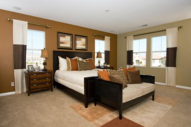
Process the image with a feature extractor and place the pixel_values on a GPU:
>>> device = torch.device("cuda" if torch.cuda.is_available() else "cpu")  # use GPU if available, otherwise use a CPU
>>> encoding = feature_extractor(image, return_tensors="pt")
>>> pixel_values = encoding.pixel_values.to(device)
Pass your input to the model and return the logits:
>>> outputs = model(pixel_values=pixel_values)
>>> logits = outputs.logits.cpu()
Next, rescale the logits to the original image size:
>>> upsampled_logits = nn.functional.interpolate(
... logits,
... size=image.size[::-1],
... mode="bilinear",
... align_corners=False,
... )
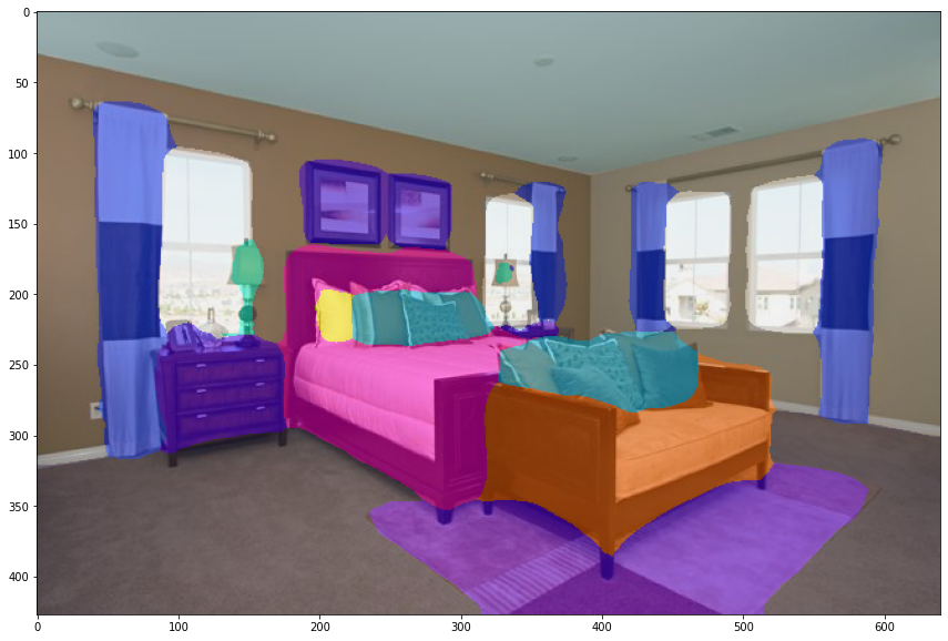
>>> pred_seg = upsampled_logits.argmax(dim=1)[0]To visualize the results, load the dataset color palette that maps each class to their RGB values. Then you can combine and plot your image and the predicted segmentation map:
>>> import matplotlib.pyplot as plt

>>> color_seg = np.zeros((pred_seg.shape[0], pred_seg.shape[1], 3), dtype=np.uint8)
>>> palette = np.array(ade_palette())
>>> for label, color in enumerate(palette):
...     color_seg[pred_seg == label, :] = color
>>> color_seg = color_seg[..., ::-1]  # convert to BGR

>>> img = np.array(image) * 0.5 + color_seg * 0.5  # plot the image with the segmentation map
>>> img = img.astype(np.uint8)

>>> plt.figure(figsize=(15, 10))
>>> plt.imshow(img)
>>> plt.show()