Two types of value-based methods

In value-based methods, we learn a value function that maps a state to the expected value of being at that state.

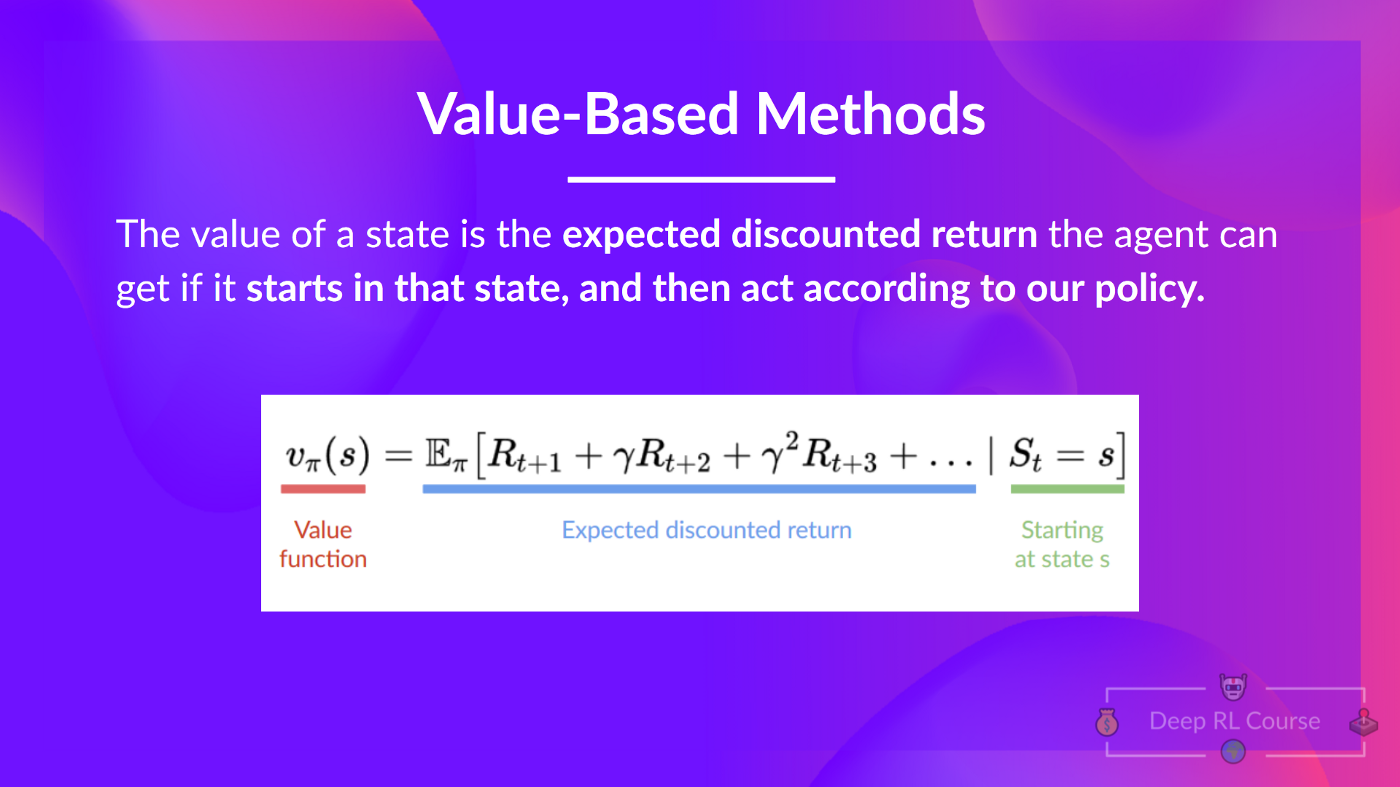
The value of a state is the expected discounted return the agent can get if it starts at that state and then acts according to our policy.

Remember that the goal of an RL agent is to have an optimal policy π*.

To find the optimal policy, we learned about two different methods:

• Policy-based methods: Directly train the policy to select what action to take given a state (or a probability distribution over actions at that state). In this case, we don’t have a value function.

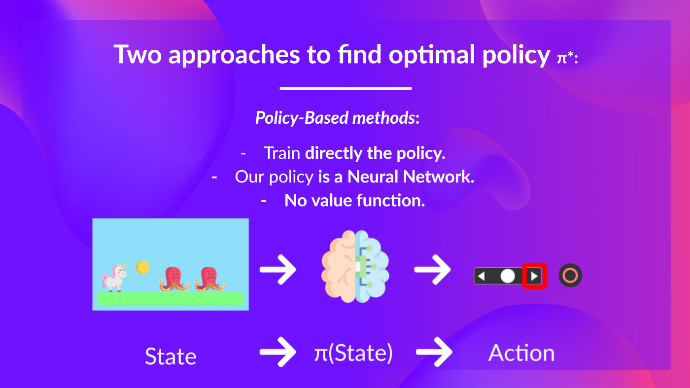
The policy takes a state as input and outputs what action to take at that state (deterministic policy: a policy that output one action given a state, contrary to stochastic policy that output a probability distribution over actions).

And consequently, we don’t define by hand the behavior of our policy; it’s the training that will define it.

• Value-based methods: Indirectly, by training a value function that outputs the value of a state or a state-action pair. Given this value function, our policy will take an action.

Since the policy is not trained/learned, we need to specify its behavior. For instance, if we want a policy that, given the value function, will take actions that always lead to the biggest reward, we’ll create a Greedy Policy.

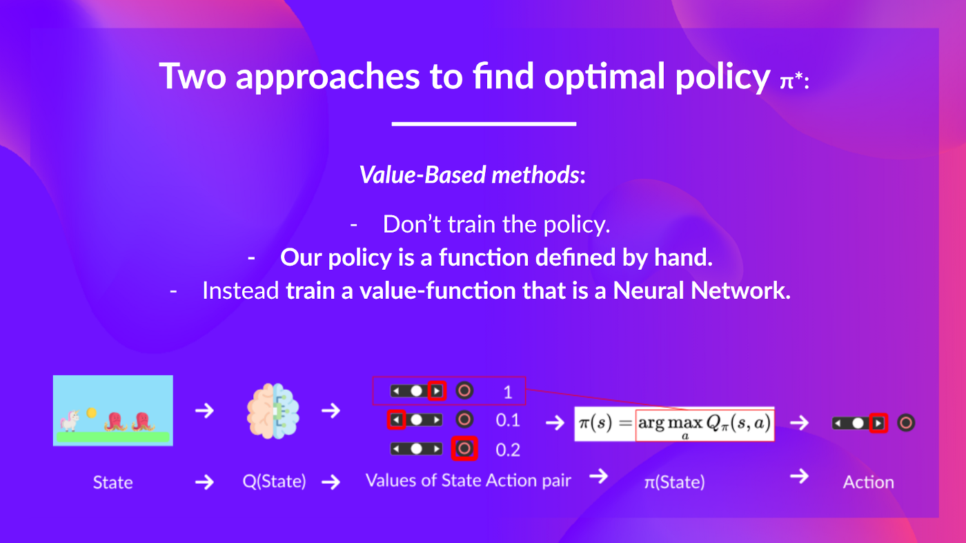
Consequently, whatever method you use to solve your problem, you will have a policy. In the case of value-based methods, you don’t train the policy: your policy is just a simple pre-specified function (for instance, the Greedy Policy) that uses the values given by the value-function to select its actions.

So the difference is:

• In policy-based training, the optimal policy (denoted π*) is found by training the policy directly.
• In value-based training, finding an optimal value function (denoted Q* or V*, we’ll study the difference below) leads to having an optimal policy.

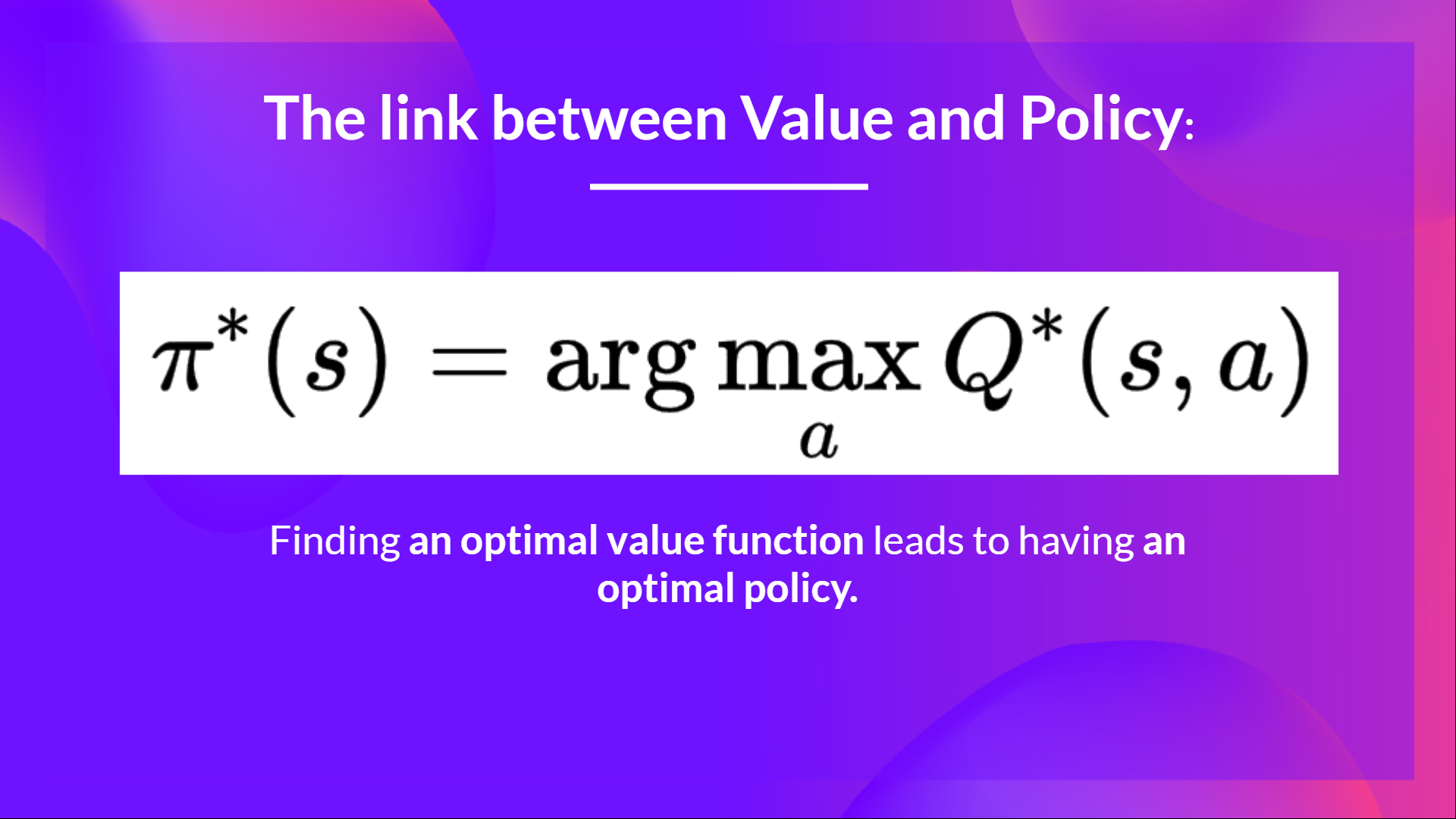
In fact, most of the time, in value-based methods, you’ll use an Epsilon-Greedy Policy that handles the exploration/exploitation trade-off; we’ll talk about this when we talk about Q-Learning in the second part of this unit.

As we mentioned above, we have two types of value-based functions:

The state-value function

We write the state value function under a policy π like this:

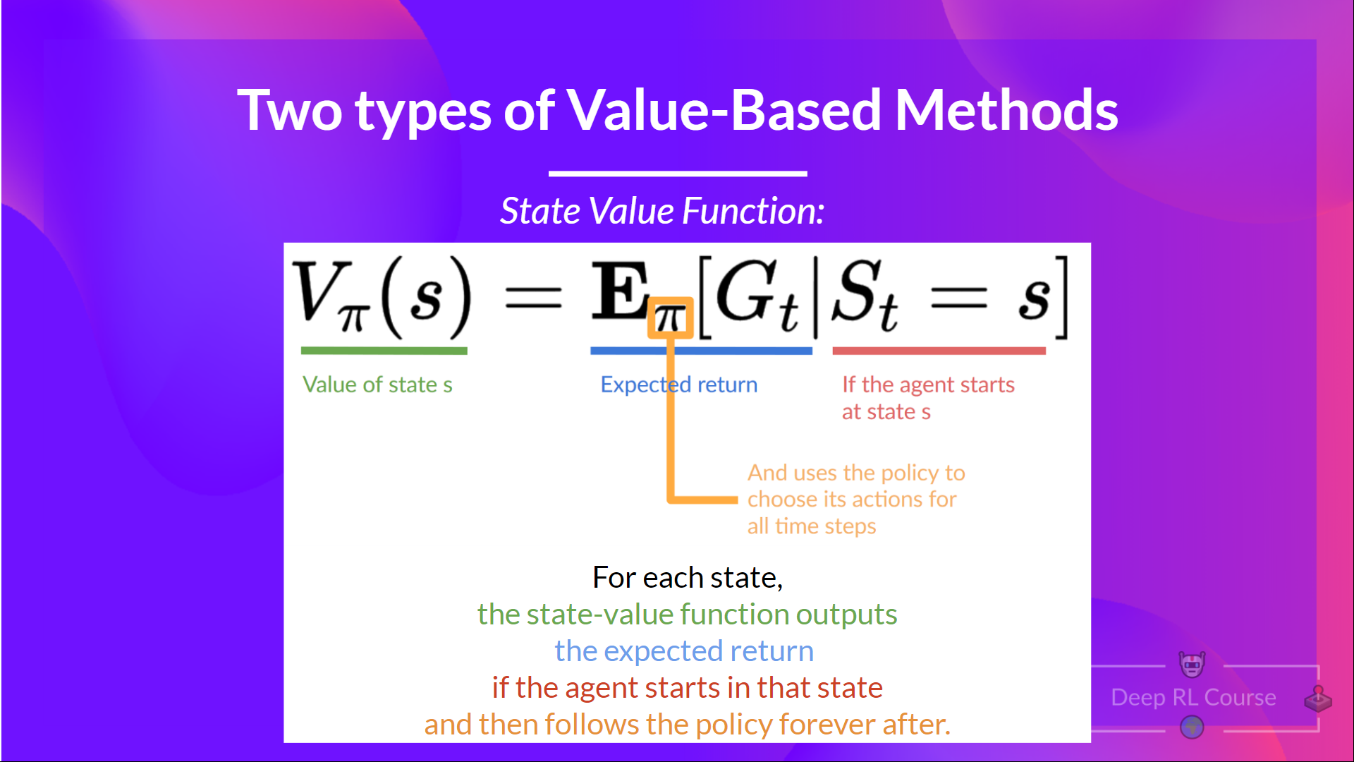
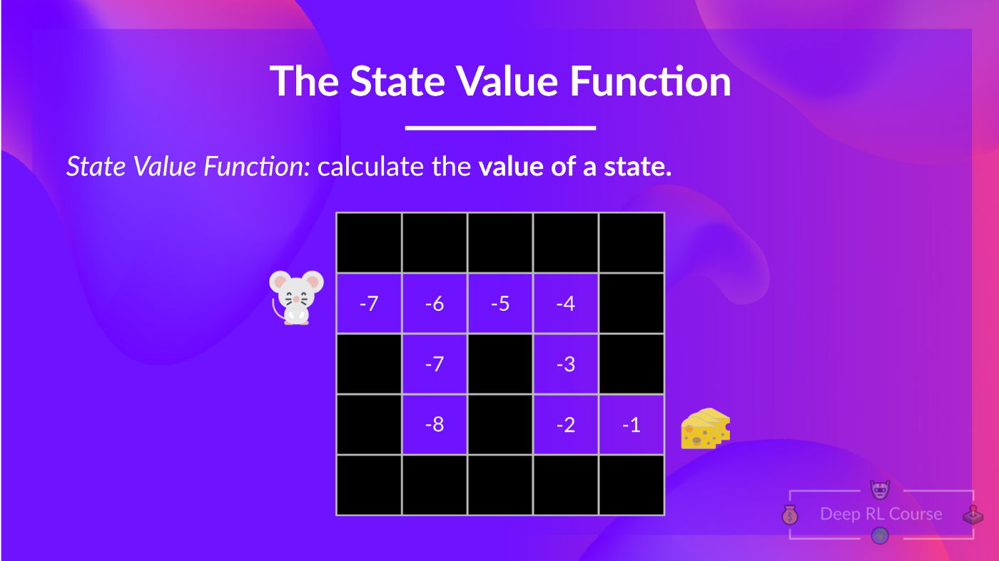
For each state, the state-value function outputs the expected return if the agent starts at that state and then follows the policy forever afterward (for all future timesteps, if you prefer).

The action-value function

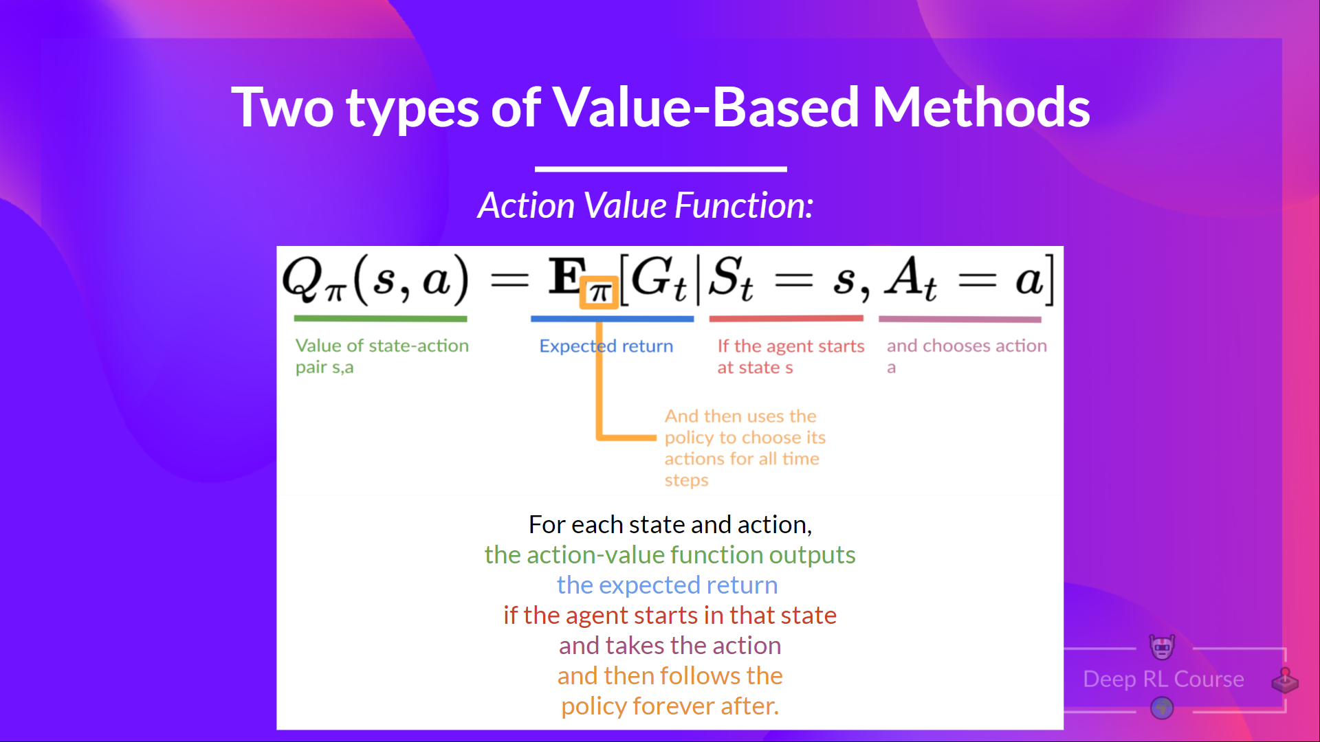
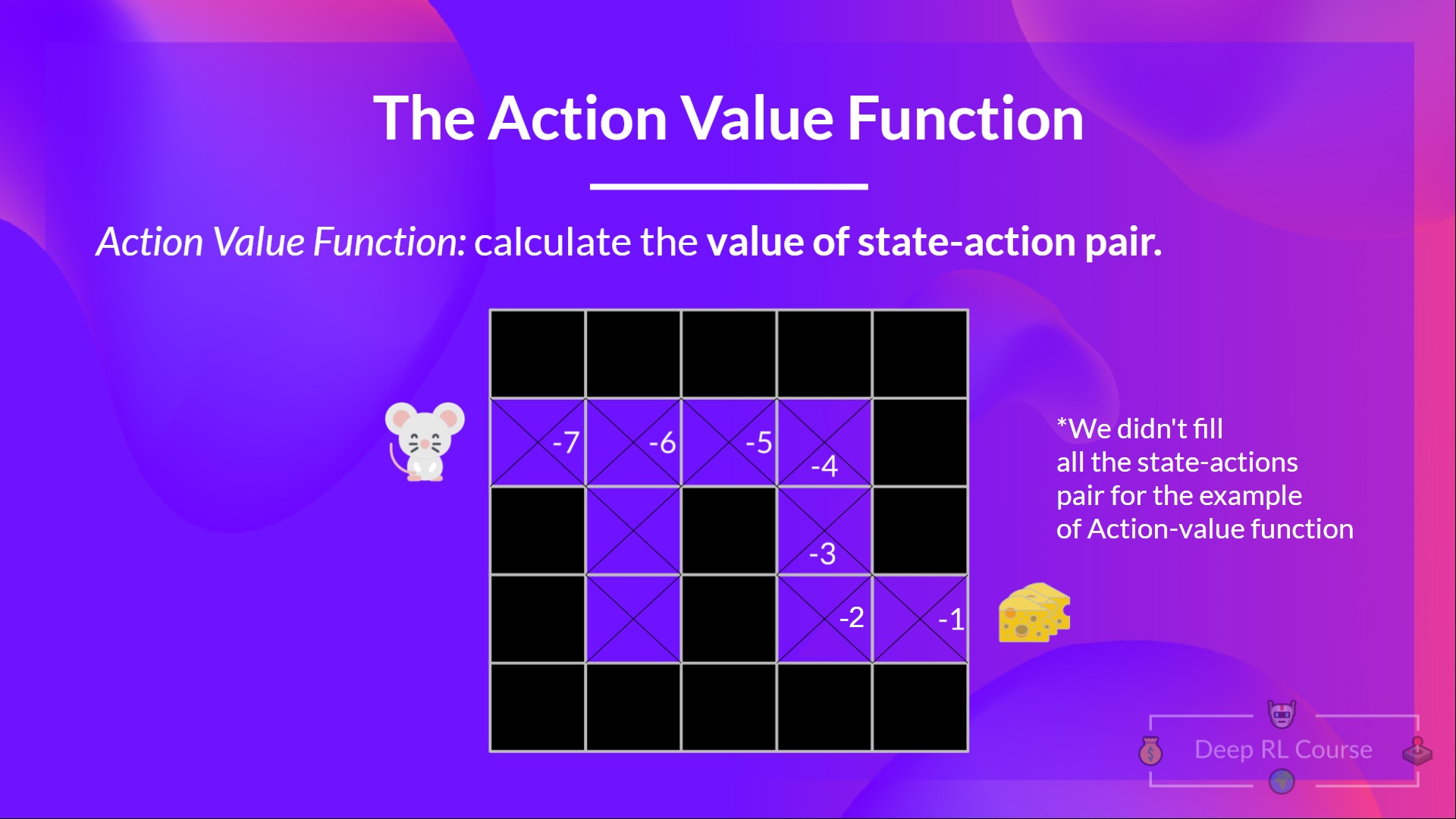
In the action-value function, for each state and action pair, the action-value function outputs the expected return if the agent starts in that state, takes that action, and then follows the policy forever after.

The value of taking action$a$ in state$s$ under a policy$π$ is:

We see that the difference is:

• For the state-value function, we calculate the value of a state$S_t$
• For the action-value function, we calculate the value of the state-action pair ($S_t, A_t$ ) hence the value of taking that action at that state.

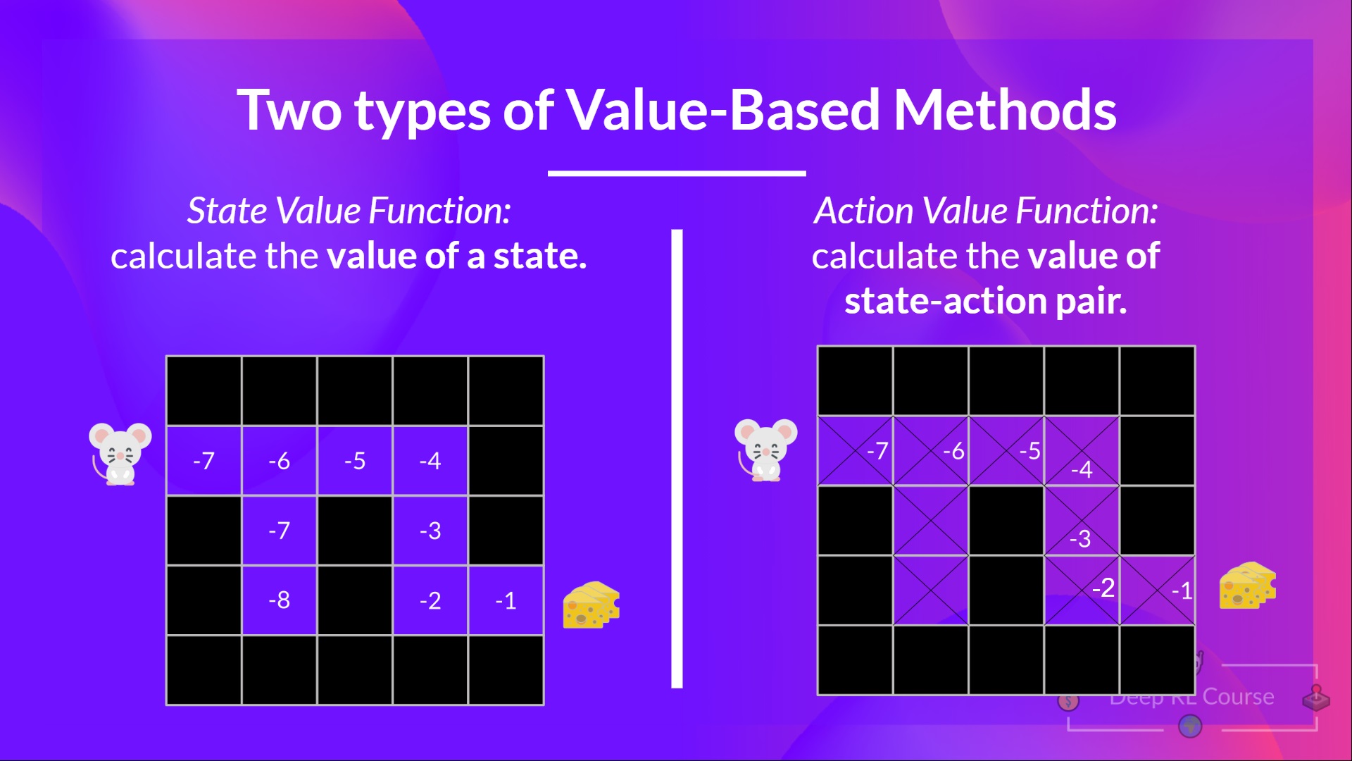
In either case, whichever value function we choose (state-value or action-value function), the returned value is the expected return.

However, the problem is that to calculate EACH value of a state or a state-action pair, we need to sum all the rewards an agent can get if it starts at that state.

This can be a computationally expensive process, and that’s where the Bellman equation comes in to help us.