Monte Carlo vs Temporal Difference Learning

The last thing we need to discuss before diving into Q-Learning is the two learning strategies.

Remember that an RL agent learns by interacting with its environment. The idea is that given the experience and the received reward, the agent will update its value function or policy.

Monte Carlo and Temporal Difference Learning are two different strategies on how to train our value function or our policy function. Both of them use experience to solve the RL problem.

On one hand, Monte Carlo uses an entire episode of experience before learning. On the other hand, Temporal Difference uses only a step ($S_t, A_t, R_{t+1}, S_{t+1}$ ) to learn.

We’ll explain both of them using a value-based method example.

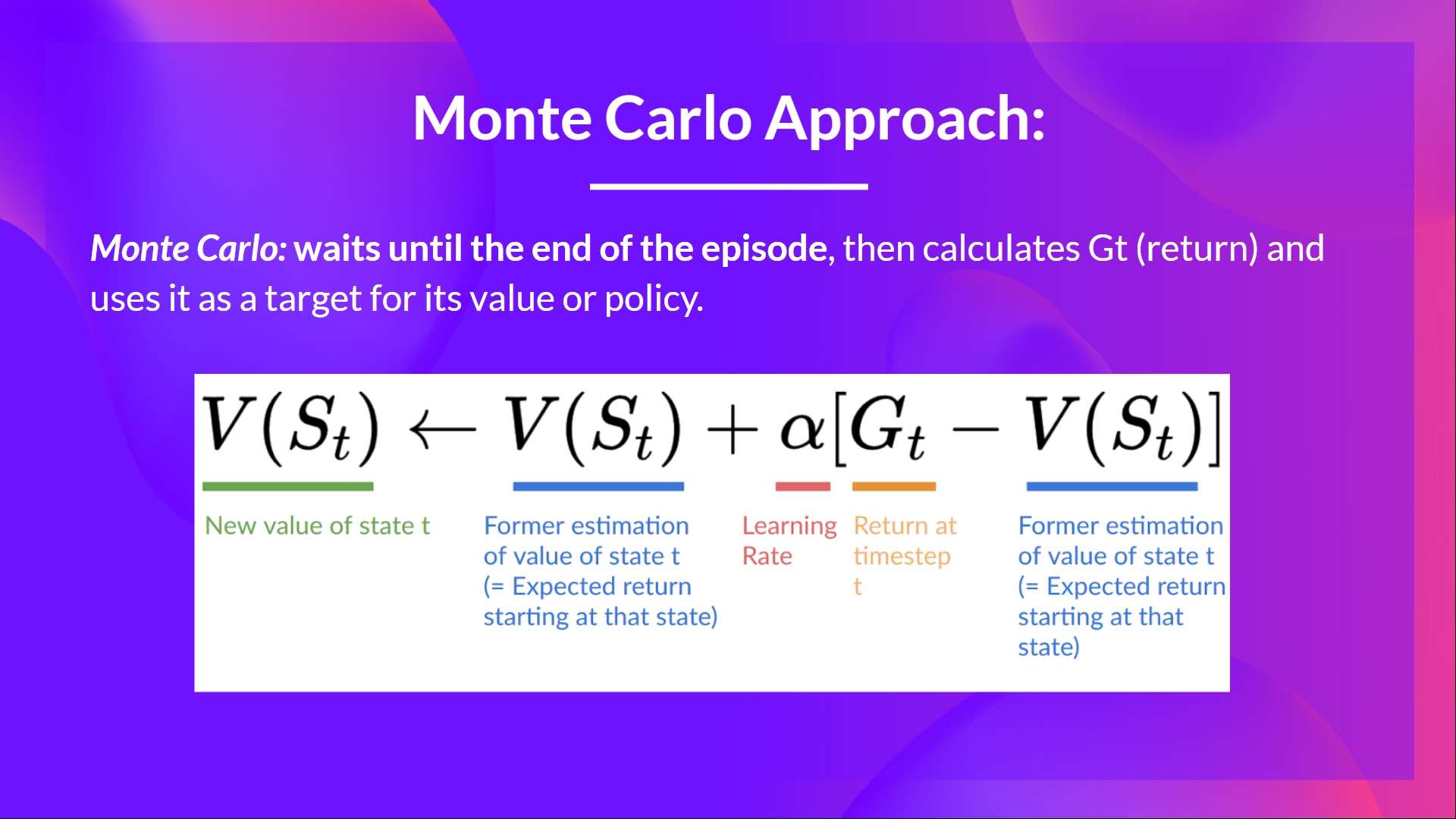
Monte Carlo: learning at the end of the episode

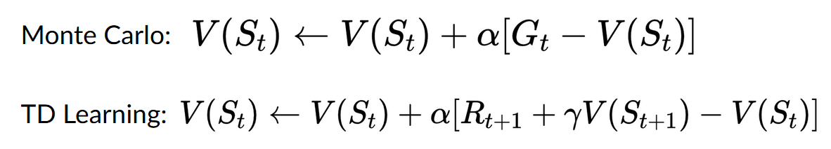
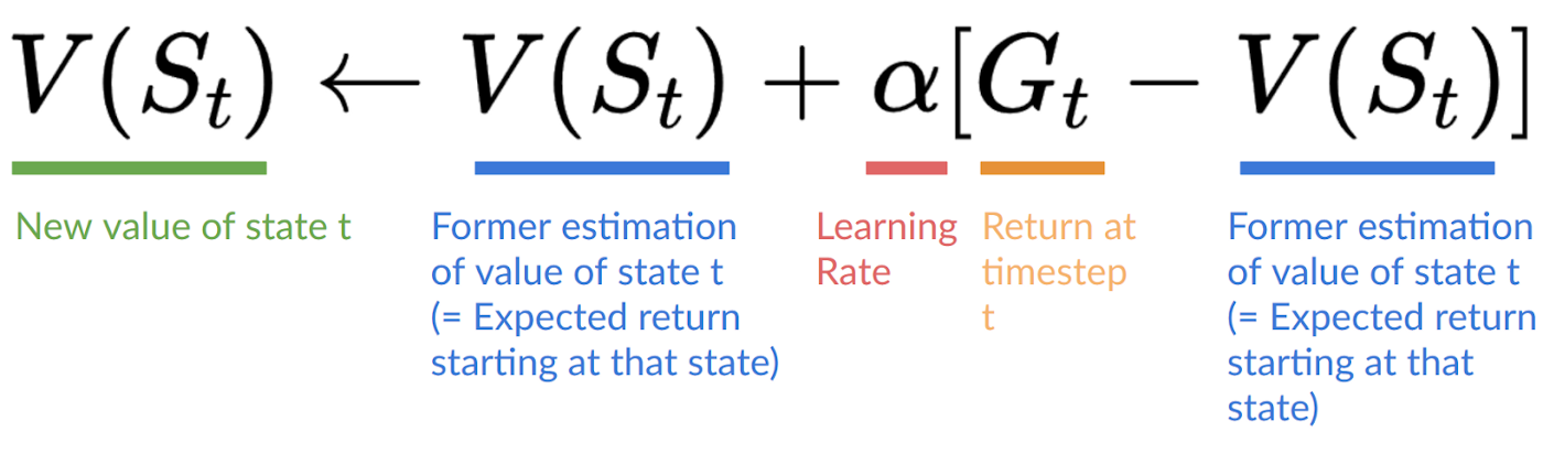
Monte Carlo waits until the end of the episode, calculates $G_t$ (return) and uses it as a target for updating $V(S_t)$.

So it requires a complete episode of interaction before updating our value function.

If we take an example:

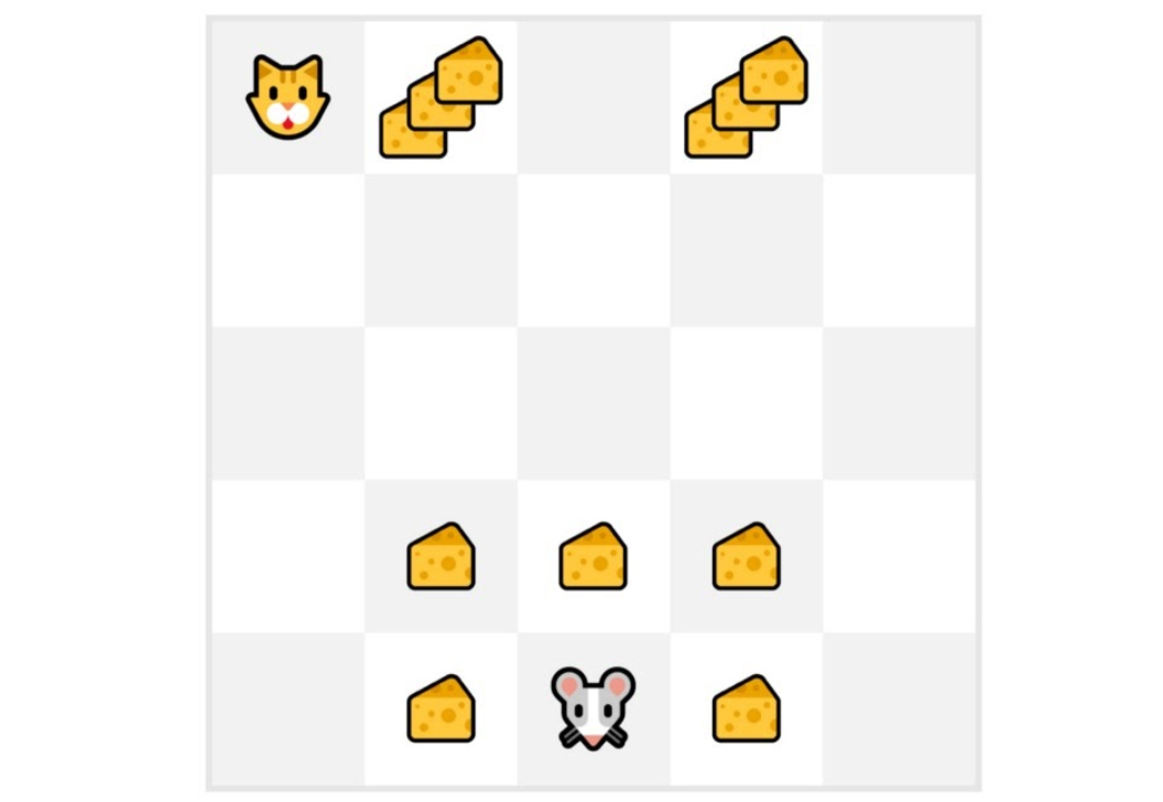
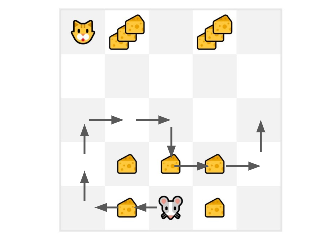
• We always start the episode at the same starting point.

• The agent takes actions using the policy. For instance, using an Epsilon Greedy Strategy, a policy that alternates between exploration (random actions) and exploitation.

• We get the reward and the next state.

• We terminate the episode if the cat eats the mouse or if the mouse moves > 10 steps.

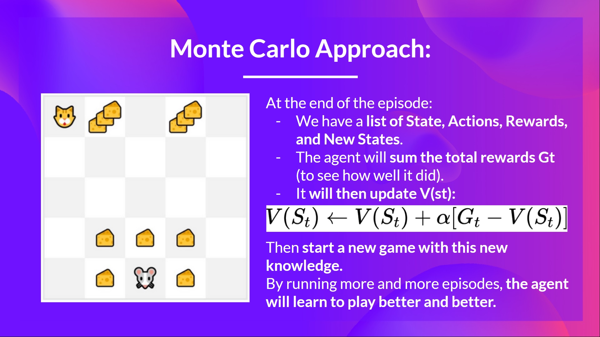
• At the end of the episode, we have a list of State, Actions, Rewards, and Next States tuples For instance [[State tile 3 bottom, Go Left, +1, State tile 2 bottom], [State tile 2 bottom, Go Left, +0, State tile 1 bottom]…]

• The agent will sum the total rewards$G_t$ (to see how well it did).

• It will then update$V(s_t)$ based on the formula

  

• Then start a new game with this new knowledge

By running more and more episodes, the agent will learn to play better and better.

For instance, if we train a state-value function using Monte Carlo:

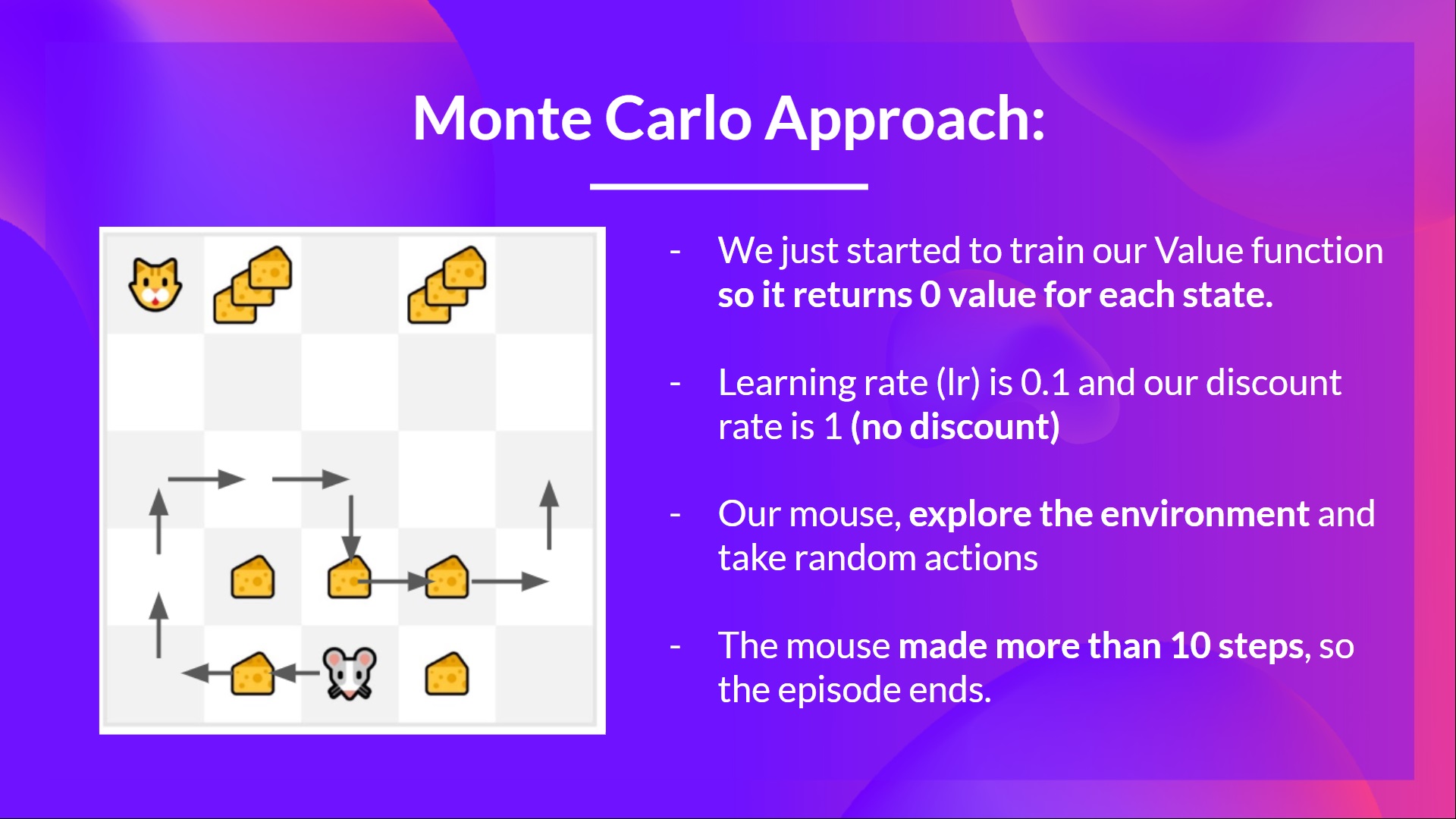
• We initialize our value function so that it returns 0 value for each state

• Our learning rate (lr) is 0.1 and our discount rate is 1 (= no discount)

• Our mouse explores the environment and takes random actions

  

• The mouse made more than 10 steps, so the episode ends .

  

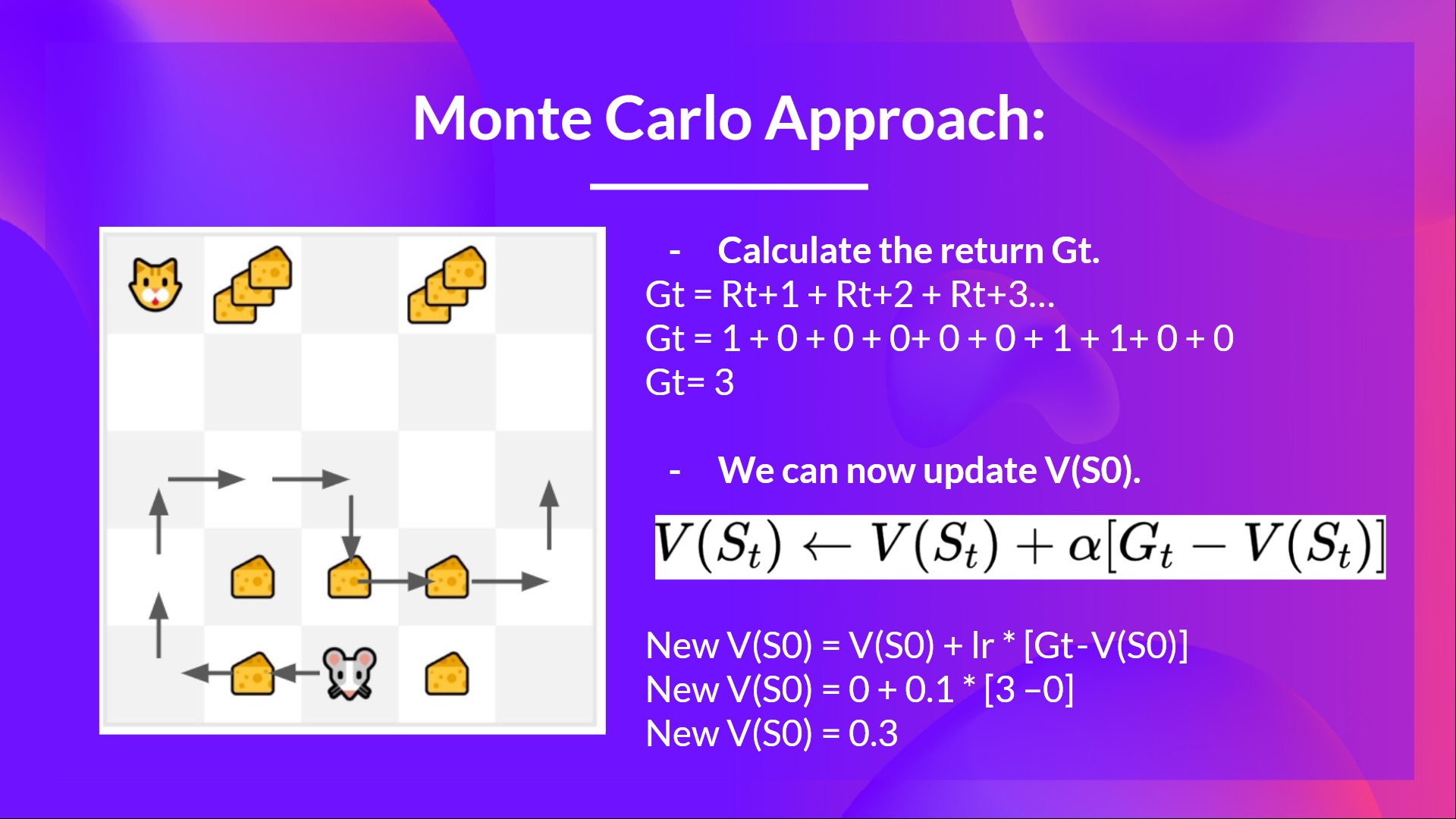
• We have a list of state, action, rewards, next_state, we need to calculate the return$G{t=0}$ $G_t = R_{t+1} + R_{t+2} + R_{t+3} ...$ (for simplicity, we don’t discount the rewards) $G_0 = R_{1} + R_{2} + R_{3}…$ $G_0 = 1 + 0 + 0 + 0 + 0 + 0 + 1 + 1 + 0 + 0$ $G_0 = 3$

• We can now compute the new$V(S_0)$:

  $V(S_0) = V(S_0) + lr * [G_0 — V(S_0)]$ $V(S_0) = 0 + 0.1 * [3 – 0]$ $V(S_0) = 0.3$

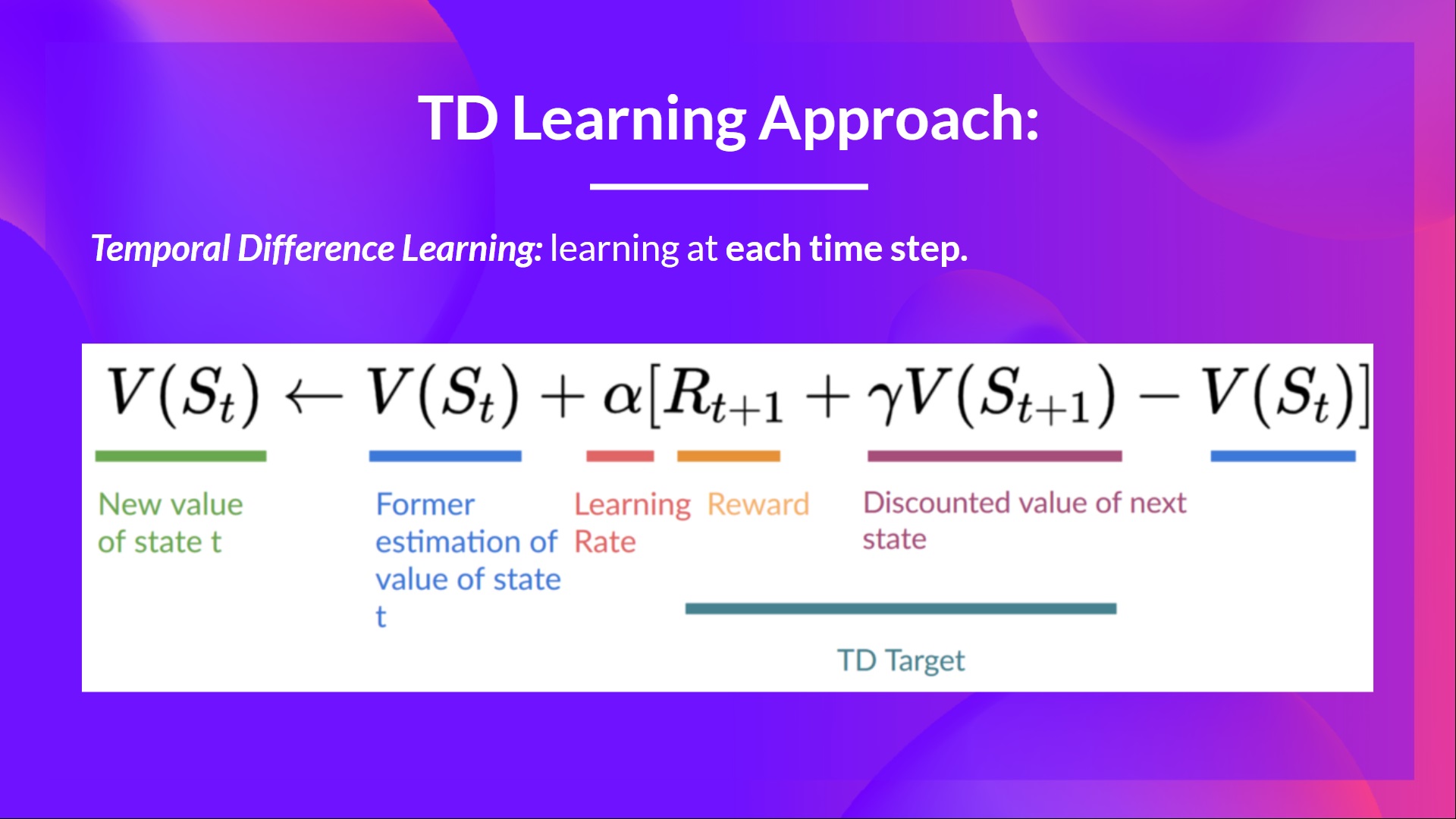
Temporal Difference Learning: learning at each step

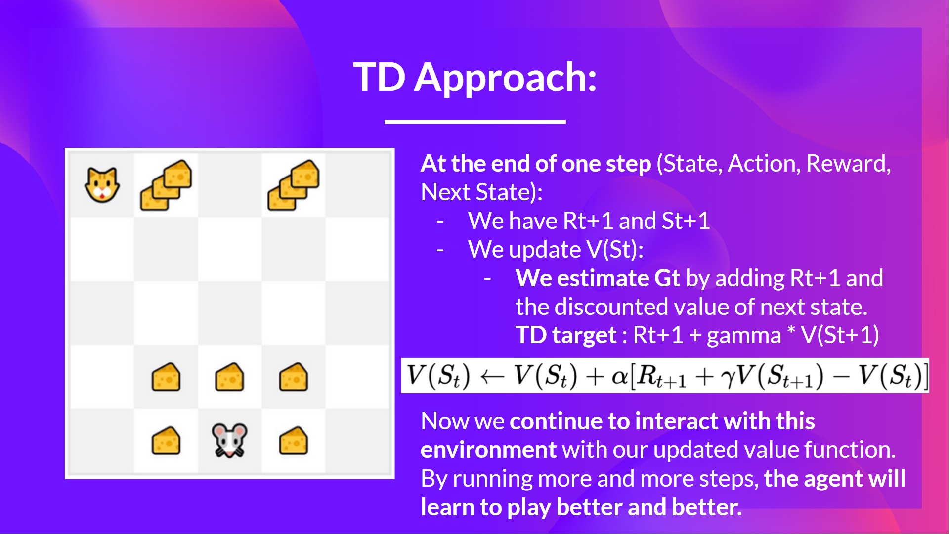
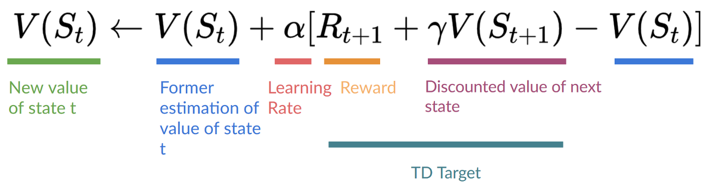
Temporal Difference, on the other hand, waits for only one interaction (one step)$S_{t+1}$ to form a TD target and update$V(S_t)$ using$R_{t+1}$ and$\gamma * V(S_{t+1})$.

The idea with TD is to update the$V(S_t)$ at each step.

But because we didn’t experience an entire episode, we don’t have$G_t$ (expected return). Instead, we estimate$G_t$ by adding$R_{t+1}$ and the discounted value of the next state.

This is called bootstrapping. It’s called this because TD bases its update in part on an existing estimate$V(S_{t+1})$ and not a complete sample$G_t$.

This method is called TD(0) or one-step TD (update the value function after any individual step).

If we take the same example,

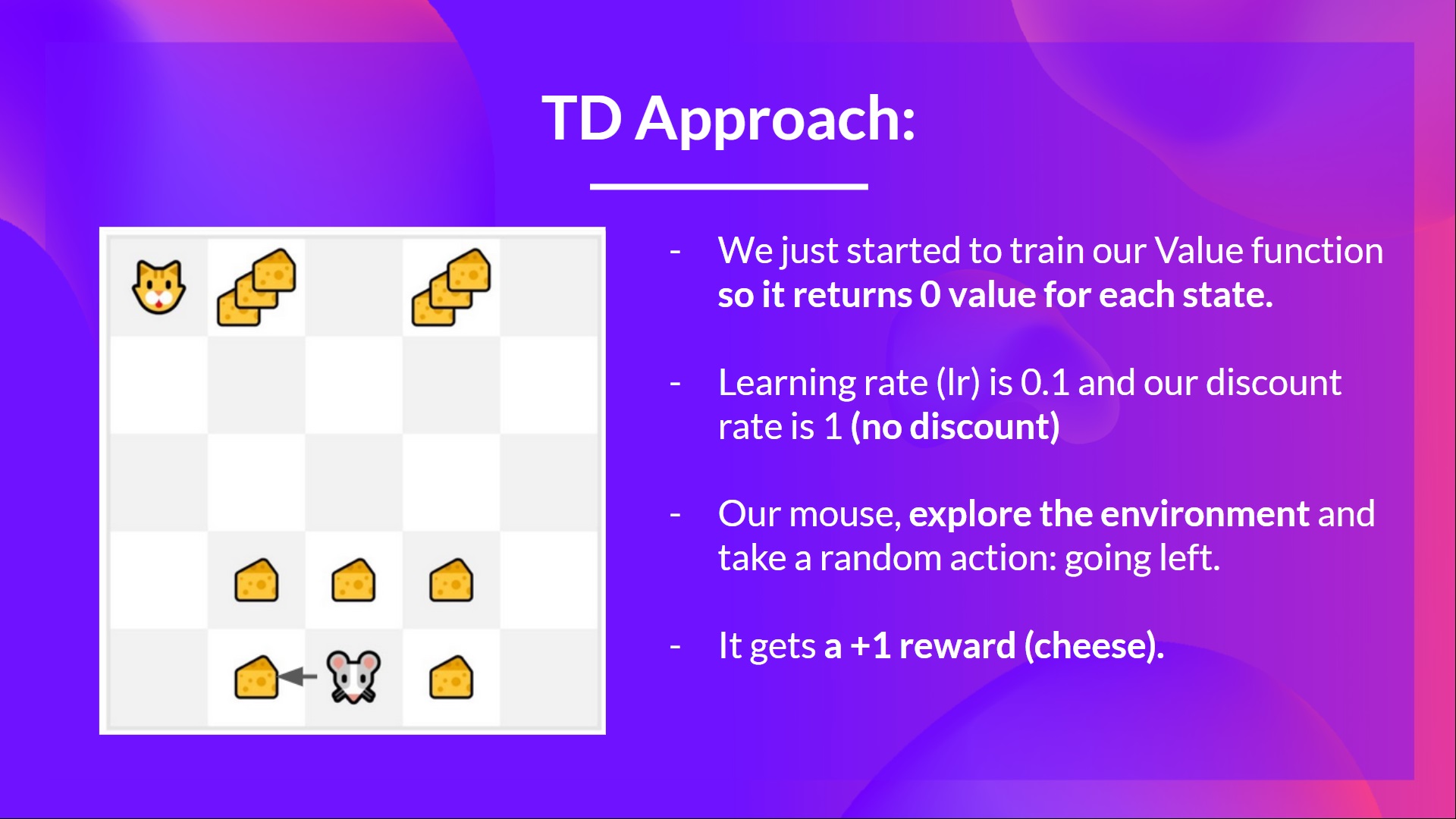
• We initialize our value function so that it returns 0 value for each state.

• Our learning rate (lr) is 0.1, and our discount rate is 1 (no discount).

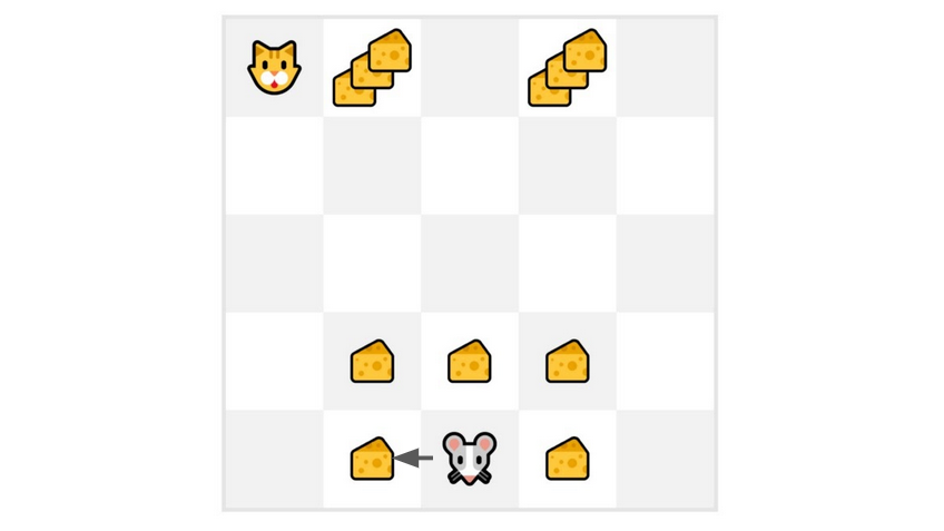
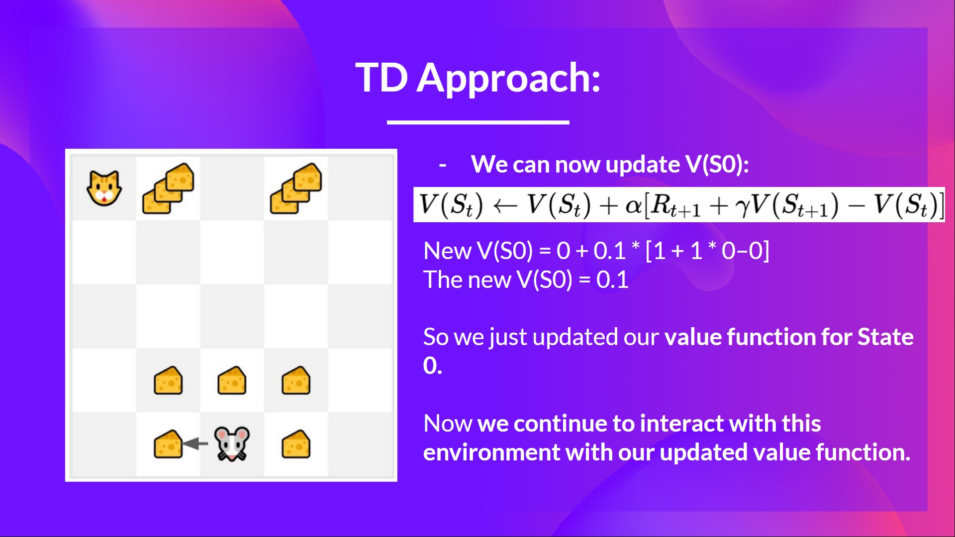
• Our mouse begins to explore the environment and takes a random action: going to the left

• It gets a reward $R_{t+1} = 1$ since it eats a piece of cheese

  

We can now update $V(S_0)$:

New $V(S_0) = V(S_0) + lr * [R_1 + \gamma * V(S_1) - V(S_0)]$

New$V(S_0) = 0 + 0.1 * [1 + 1 * 0–0]$

New$V(S_0) = 0.1$

So we just updated our value function for State 0.

Now we continue to interact with this environment with our updated value function.

To summarize:

• With Monte Carlo, we update the value function from a complete episode, and so we use the actual accurate discounted return of this episode.

• With TD Learning, we update the value function from a step, and we replace$G_t$, which we don’t know, with an estimated return called the TD target.