
GANs for tabular data
Authors
- Tomer Shahar - Tomer Shahar
- Nevo Itzhak - Nevo Itzhak
Introduction
In this assignment, we were given two tasks:
(1) create a Generative Adversarial Network (GAN) that can produce tabular samples from two given datasets, and
(2) build a general generative model that receives a black-box as a discriminator and can still generate samples from the tabular data. This is done by attempting to predict the scores given by the black-box model.
We implemented this assignment using mainly Keras and Sklearn.
Dataset Analysis
- Two tabular files.
- The first one (Adult.arff) contains
- 15 columns
- 6 numeric columns
- 9 nominal columns
- ~32,500 instances
- 15 columns
- The second one (bank-full.arff) contains
- 17 columns
- 7 numeric columns
- 10 nominal columns
- ~45,000 instances
- 17 columns
An example for the ‘Adults’ dataset:

An example for the ‘Bank-full’ dataset:

Code Design:
Our code consists of three scripts:
- nt_exp.py - the script that runs the experiments to find the optimal parameters for our GAN network.
- nt_gan.py - defines the GAN class, training and testing the models.
- nt_gg.py - defines the general generator class, training and testing the models.
Generative Adversarial Networks (Part 1)
Architecture:
We used a fairly standard architecture for both the generator and discriminator.
Generator:
| Layer # | Layer Type | Input Size | Activation Function |
Notes |
|---|---|---|---|---|
| 1 | Noise | int(x/2) Where x is the number of features in the dataset |
- | |
| 2 | Dense | x*2 | LeakyReLU |
|
| 3 | Dense | x*4 | LeakyReLU |
Has a dropout (see details below) |
| 4 | Dense | x*2 | LeakyReLU |
Has a dropout (see details below) |
| 5 | Output | x | Sigmoid |
Discriminator:
| Layer # | Layer Type | Input Size | Activation Function |
Notes |
|---|---|---|---|---|
| 1 | Input | x Where x is the number of features in the dataset |
- | |
| 2 | Dense | x*2 | LeakyReLU |
|
| 3 | Dense | x*4 | LeakyReLU |
Has a dropout (see details below) |
| 4 | Dense | x*2 | LeakyReLU |
Has a dropout (see details below) |
| 5 | Output | 1 | Sigmoid |
Results Evaluation:
We devised a few metrics to judge our models:
- Mean Minimum Euclidean Distance - This approach finds for each generated record the similar record in the real data and compute euclidean distance between them. Then, the metrics compute the mean of all of these distances. We want low values of this metric for the fooled samples and higher values of this metric for not fooled samples.
- Principal Components Analysis (PCA) Distribution -This approach transforms the original data to PCA with two components and then does the same thing to the fooled and not fooled samples. We can understand from the output plot three things:
- How similar the fooled samples are to the real data.
- How similar the not fooled samples are to the real data.
- How similar the fooled and the not fooled samples are.
- Understand how the discriminator decides whether or not a sample is real or not.
Network Hyper-Parameters Tuning:
NOTE: Here we explain the reasons behind the choices of the parameters.
After implementing our GAN, we optimized the different parameters used. Some parameters, like the batch size, it is very hard to predict what will work best so this method is the best way to find good values to use.
We tested the parameters based on the first metric we presented - mean minimum euclidean distance.
MMDF = Mean minimum euclidean distance for the fooled samples
MMDNF = Mean minimum euclidean distance for the not fooled samples
MMDG = MMDF - MMDNF
NFL = Number of not fooled samples out of the 100 generated samples.
W1 = 0.33 (weight)
W2 = 0.33 (weight)
W3 = 0.34 (weight)
We use the following metric to determine the parameters:
NTSCORE = w1 * (MMDF + MMDNF) + w2 * (MMDG) + w3 * (NFL/100)
- In the first component (MMDF + MMDNF), we want the distance of both MMDF and MMDNF to be low (checks the generator).
- In the second component (MMDG), we want the gap between MMDF and MMDNF to be greater than zero. In other words, MMDNF need to be smaller than MMDF (checks the discriminator).
- In the third part (NFL\100), we need the NFL to be low as possible (checks the generator).
The lower the value of this score, the better the model is.
Each combination takes a long time to train (5-15 minutes) so we tried only a few values for each parameter:
- Learning Rate: We tried different values, ranging from 0.1 to 0.0001.
- Epochs: We tried epochs of 5, 10 and 15.
- Batch size: We tried 64, 128, and 1024.
- ReLU alpha: We tried 0.2 and 0.5.
- Dropout: We tried 0.3 and 0.5.
- After running numerous experiments, we found:
- For the adults dataset, these parameters worked best:
- Learning Rate: 0.001
- Epochs: 10
- Batch Size: 128
- Alpha: 0.5
- Dropout: 0.5
- For the bank-full dataset, these parameters worked best:
- Learning Rate: 0.001
- Epochs: 10
- Batch Size: 128
- Alpha: 0.2
- Dropout: 0.3
- For the adults dataset, these parameters worked best:
- We tried all of the possible combinations of the parameters detailed above which led to a huge number of experiments but led to us finding the optimal settings which were used in the section below.
Experimental Results:
The best results are in bold -
For adults dataset, the results of the model were:
- MMDF (Mean minimum euclidean distance for the fooled samples) was 0.373
- MMDNF = Mean minimum euclidean distance for the not fooled samples was 0.422
- Several samples that “fooled” the detector:

- Several samples that “not fooled” the detector:

- Plotting the PCA shows that the fooled samples are very similar to the real data and the not fooled samples are less similar.

- Out of 100 samples, 74 samples were fooled by the discriminator and 26 samples were not fooled by the discriminator.
- A graph describing the loss of the generator and the discriminator:
- The models went back and forth with their losses, although the discriminator was lower than the generator most of the time.
- The generator loss was extremely decreased while the discriminator loss was quite the same.
- Eventually the generator and the discriminator were quite coveraged nearly a loss of 0.6.

For bank-full dataset, the results of the model were:
- MMDF (Mean minimum euclidean distance for the fooled samples) was 0.262645066
- MMDNF = Mean minimum euclidean distance for the not fooled samples was 0.305854238
- Several samples that “fooled” the detector:

- Several samples that “not fooled” the detector:

- Plotting the PCA shows that the fooled samples are very similar to the real data and the not fooled samples are less similar.

- Out of 100 samples, 32 samples were fooled by the discriminator and 68 samples were not fooled by the discriminator.
- A graph describing the loss of the generator and the discriminator:
- The model went back and forth with their losses, although the discriminator was always lower than the generator.
- The generator loss was extremely decreased while the discriminator loss was quite the same.
- Eventually the generator and the discriminator were coveraged nearly a loss of 0.5.

General Generator (Part 2)
In this section we were tasked with creating a blackbox discriminator (in our case, a random-forest model) and to create only a generator that can create samples based on the confidence scores given by the blackbox discriminator. As before, the input for the generator is a vector of random noise, but in addition to that we also provided it with a sample of the probability given by the blackbox model to class 1 (there are only 2 classes so the probabilities simply sum to 1). The goal is for the generator to learn the distribution of the probabilities in addition to creating good synthetic samples.
Architecture:
We used nearly the same generator architecture coupled with the default values for Random Forest.
Generator:
| Layer # | Layer Type | Input Size | Activation Function |
Notes |
|---|---|---|---|---|
| 1 | Noise (Input) | int(x/2) + 1 Where x is the number of features in the dataset |
- | +1 for the desired confidence. |
| 2 | Dense | x*2 | LeakyReLU |
|
| 3 | Dense | x*4 | LeakyReLU |
Has dropout |
| 4 | Dense | x*2 | LeakyReLU |
Has dropout |
| 5 | Output | x | Sigmoid | Loss - Categorical Cross Entropy |
Training Phase
The generator must be given a desired probability and then generate a sample that indeed results in that probability from the blackbox model. Therefore, it must be punished when the probability is far from what we wanted. This is the process:
- The generator creates N samples (based on batch size). The last column is the probability for a single class (class 1 in our case).
- These samples are fed to the (trained) discriminator which outputs probabilities for each class.
- We aim to mimic these probabilities, so in addition to a noise vector they are fed into the generator.
- We then run it through the generator, where the loss function is the binary cross entropy calculated between the probability given and the probability of each sample created.
- The weights are adjusted accordingly and a new batch is generated.
Network Hyper-Parameters Tuning:
As before, we did hyper parameter tuning to achieve the best results. We tried various combinations:
- Learning Rate: We tried different values, ranging from 0.1 to 0.0001.
- Epochs: We tried epochs of 5, 10 and 15.
- Batch size: We tried 64, 128, and 1024.
- ReLU alpha: We tried 0.2 and 0.5.
- Dropout: We tried 0.3 and 0.5.
- After running numerous experiments, we found that, these parameters works best:
- Learning Rate: 0.001
- Epochs: 10
- Batch Size: 128
- Alpha: 0.2
- Dropout: 0.3
Results Evaluation:
In this part the main goal was for the distribution of confidence probabilities to distribute uniformly, since we sampled 1000 confidence scores uniformly as required. A good model should be one that indeed results in such a distribution. We designated the last column as the label. It must be noted, however, that the classes are imbalanced in the ‘adult’ dataset (about 75% of the data is class 1 while 25% is class 0).
Adult dataset:
Accuracy: 0.859
Class 0 - Min confidence: 0.0 - Max Confidence: 1.0 - Mean confidence: 0.253
Class 1 - Min confidence: 0.0 - Max Confidence: 1.0 - Mean confidence: 0.747
Class distribution:

- Note that there is some imbalance here, which is nearly identical to the ratio between the mean confidence scores for each class.
- Probability distribution for class 0 and class 1, for the test set:


- Note that the images mirror each other.
Bank Data set:
- Accuracy: 0.903
- Class 0 - Min confidence: 0.0 - Max Confidence: 0.96 - Mean confidence: 0.118
- Class 1 - Min confidence: 0.04 - Max Confidence: 1.0 - Mean confidence: 0.882
Class distribution:

- The data here is even more imbalanced. The confidence scores reflect this.
- Confidence score distribution for test set:


Generator Results:
Here we first uniformly sampled 1000 confidence rates from [0,1]. Then, based on these rates we generated 1,000 samples. The goal being that the discriminators confidence rate also distributed uniformly. This is of course a hard task considering how skewed the confidence rate is, as seen above, since class 1 is much more likely (3 times more for the first data set and 8 times more for the second one).
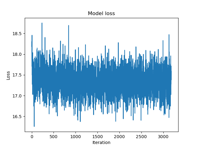
Adult Dataset:
- Training loss:

Confidence score distribution for each class:
- Note that they mirror each other.
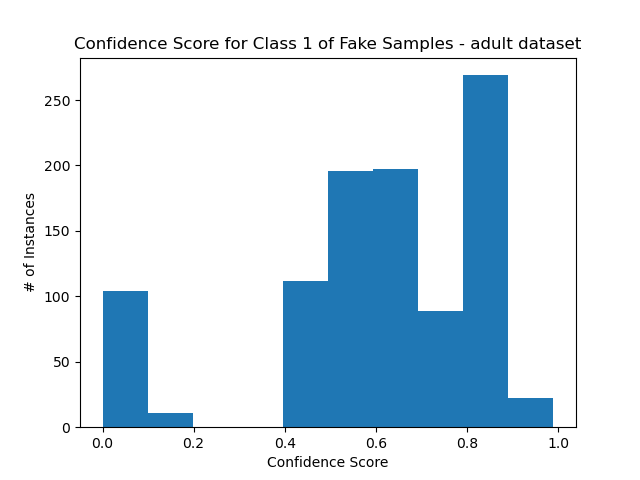
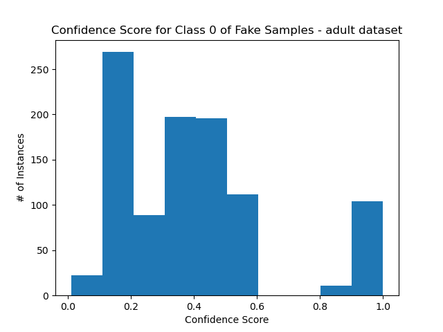
- The results are far from uniform, but it is obvious that they are skewed towards the original confidence scores.
Error rates for class 1:
- Note how the greatest error rate is for low probabilities. This is in line with the results we saw earlier, where the discriminator tends to favor class 1. As you can see, the lowest errors were for 0.8~ desired confidence rates. This is close to the mean confidence for class 1.

- Note how the greatest error rate is for low probabilities. This is in line with the results we saw earlier, where the discriminator tends to favor class 1. As you can see, the lowest errors were for 0.8~ desired confidence rates. This is close to the mean confidence for class 1.


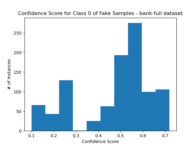
Bank Dataset:
Training loss:
Confidence score distribution for each class:
- As before, they mirror each other.
- The distribution isn’t uniform, and is slightly skewed in the opposite direction of the distribution for the test set.

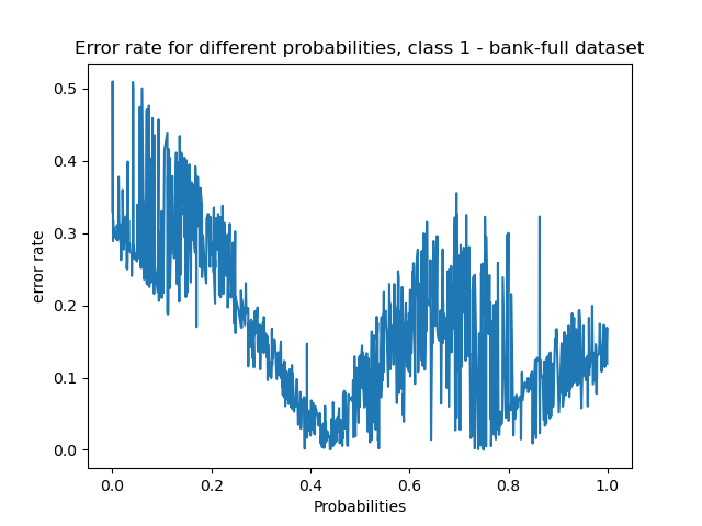
Error rates for class 1:
- The lowest error rates were achieved for probabilities of around 0.4~. The highest was for probability of 0.


Discussion
For the adult dataset, the confidence rates for the generated samples are not completely random, but not uniformly distributed. But it is clear that it skews towards the original distribution, which makes sense. However, this is not the case for the bank dataset. Perhaps this can be explained with the high loss rate and the extreme imbalance in the original data.
For both datasets, our generator indeed suffered from mode collapse and only generated samples from the class with more instances in the training set. This obviously hindered the results. Since only class 1 was generated, obviously we only have results for that one so it is difficult to compare results between classes. Perhaps a better approach would be to generate synthetic samples (e.g, SMOTE) to ensure better training data, or choose a feature that distributes more evenly.