RNNs & LSTMs Explained with Example
By Michael Peres
28th May 2024
Introduction
I recently started looking for solutions related to sequential data for audio, and although I understand transformers, I wanted to appreciate the work done by RNNs and LSTMs. Thus, this repo and work is related to the tutorial and expand my knowledge to a practical implementation. For my dissertation, three models are created, a CNN, TinyViT model and a LSTM model. However, I was not aware of the technology and operations necessary with LSTMs. Aiming to remember and obtain some implementation skillset, I aim to create a simple LSTM model for a simple task, and document my understanding during the process.
I would like to also note some resources that made this straightforward to grasp,
RNNs
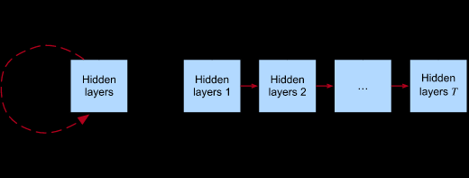
RNNs work with data of variable time lengths T, in which for each time step, the forward propagation is calculated and updates the same weights recursively, hence the name.
The initial block shows this recursion, but in other contexts we may want to unroll this operation across time steps providing a kind of transition between hidden layers.
We learn more about the problems with RNNs due to this sharing of a hidden state on the vanishing and exploding gradients problems.
But before this, we should understand one concept from RNNs, that I learned via the D2L book, that is the idea of Markov Order Model, which is that if we imagine we have a sequence of length 1-T and we want to predict T+1, then the Markov Order Model states the number of previous time steps needed tau, in order to accurately predict the next time step, such that any further removal of historical timesteps will not effect the overall loss of the model.
For example, if we have a stock price of 10 days of TSCO, and we aim to predict the stock price on the eleventh day, we could use all 10 previous days, and achieve a 90% accuracy, however if we have a model that can predict using 4 historical days, and still have 90% accuracy, such that if we go to 3 days it falls, then we can state this model follows a 4th order Markov Model.
Main Idea
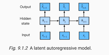
The main idea of RNNs is that we work with both an input and a hidden state, such that in reality, the probability of the next word is dependent on the previous hidden state rather than the previous time steps, saving space, and not making a model that is dependant on the size of the sequence.
For example:
P(x_t=1 | x_t-1, x_t-2, x_t-3) ~~ P(x_t=1 | h_t-1)
I put a "~" for approximation, but in reality can be near equal, if the function is strong enough to represent it.
The book goes through some examples of teaching a Linear regression model to use 4 previous time steps to predict the next time step, and the results are quite good, but the main issue is that the model is not able to learn long term dependencies (failing when it comes to k steps prediction), and this is where LSTMs come in.
The first thing with RNNs is that we obtain a function that updates the hidden state based on the input at time t and the previous hidden state at time t-1.
In RNNs we have three different types of weights, which depend on 3 different parameters,
- W_xh: Weights for the input (d,h)
- W_hh: Weights for the hidden state (h,h)
- b_h: Bias for the hidden state (h,)
- W_hq: Weights for the output (h,q)
(n being the batch size, d being the input dimension, h being the hidden dimension, and q being the output dimension) Here we need the input dimension, which usually, will be of dimensions n,d Hidden state being a vector h of dimensions n,h Output being a vector q of dimensions n,q
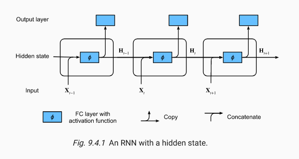
The two main equations of RNNs being.
(1) to update the hidden state,
(2) To calculate the output from hidden state and weight w_hq.
The diagram shows this flow, where the hidden state persists updating,
For the RNN part, implementation file has been added, namely RNN_Scratch.py & RNN.py, with an example followed from PyTorch.
However, as mentioned before, there are problems with RNNs, notably the vanishing and exploding gradients problem.
Vanishing and Exploding Gradients of RNNs
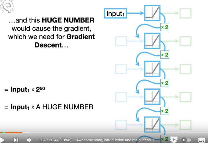
The main idea of exploding gradients, was highlighted by this video, and its to do with the recurrent weights above 1,
Such that recursively multiplication of above causes the model have large gradients, moving it out of a the gradient slope, and possibly ruining any current progress, similar to a large learning rate.
The same can be said for weights less than 1, say 0.5, which eventually go to 0, making that specific weights effect on overall model close to 0, and making it hard or backpropagation to learn from it.
LSTMs
LSTMs are a noticeable solution to this, although I do not see this, the D2L book mentions the calculation of loss, and could aim to help understand how LSTMs aid in this problem.
However, I did not bother, as current time constraints on dissertation.
The main idea of LSTMs seems confusing at the start and made no sense to me, however with some time, the video to start with and then the book to solidify, it becomes quite trivial and even easier to implement.
The solution uses both short term and long-term memory in the form of two rolling values (persistently used through time steps), a internal state (long term) and a hidden state (short term).
We need to remember to key things before going forward, activation functions:
- Sigmoid:
1/(1+e^-x)
The sigmoid function is used to squish the values between 0 - 1, and is used to gate the information flow. It generates a value from 0 to 1, and we will explain what this is used for (filtering).
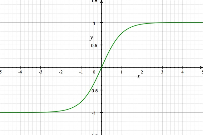
- Tanh:
(e^x - e^-x)/(e^x + e^-x)
The tanh function is used to squish the values between -1 - 1, and is used to gate the information flow. (Value generation)
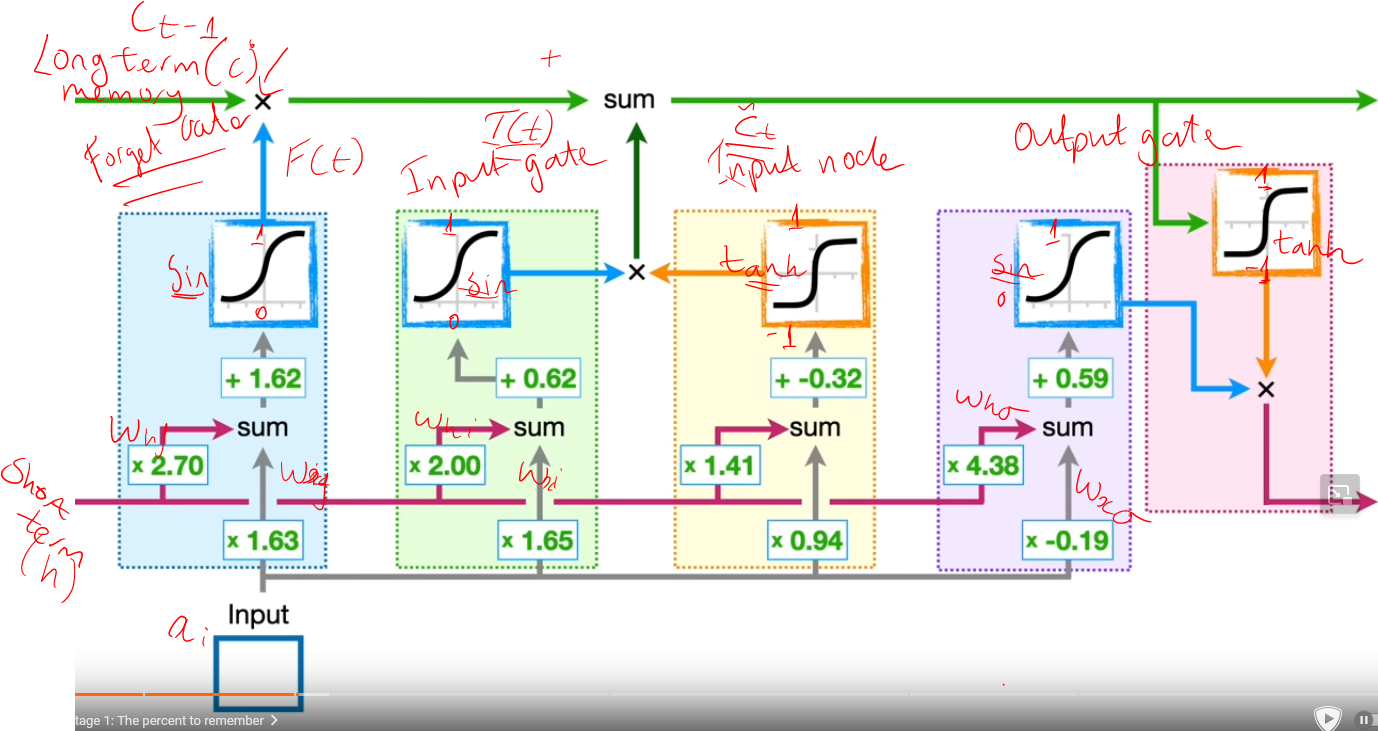
LTSMs are very simple, for instance, we have three gates and I will explain this all, here is an overview of the LSTM cell, with some annatations.
There are 3 different gates, which are the forget gate, input gate, and output gate.
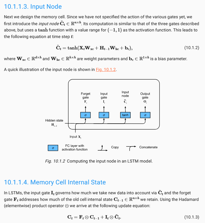
The gates can be calculated to input the internal state, with the following equations:
The forget gate, states how much of the current long-term memory is remembered, as a percentage of 0-1, which is multiplied by the previous long term memory.
The input gate takes both a percentage (sin) and value (-1 to 1, tanh) to add to the value. The output gate is the final output, which is a squished version of the internal state, to be used as the hidden state.
Here is another daigram showing the same thing, it's quite simple to use,
We will now implement the LSTM model in the LSTM_Scratch.py file, and LSTM.py torch implementation.
