Datasets documentation
Semantic segmentation
Semantic segmentation
Semantic segmentation datasets are used to train a model to classify every pixel in an image. There are a wide variety of applications enabled by these datasets such as background removal from images, stylizing images, or scene understanding for autonomous driving. This guide will show you how to apply transformations to an image segmentation dataset.
Before you start, make sure you have up-to-date versions of albumentations and cv2 installed:
pip install -U albumentations opencv-python
Albumentations is a Python library for performing data augmentation for computer vision. It supports various computer vision tasks such as image classification, object detection, segmentation, and keypoint estimation.
This guide uses the Scene Parsing dataset for segmenting and parsing an image into different image regions associated with semantic categories, such as sky, road, person, and bed.
Load the train split of the dataset and take a look at an example:
>>> from datasets import load_dataset

>>> dataset = load_dataset("scene_parse_150", split="train")
>>> index = 10
>>> dataset[index]
{'image': <PIL.JpegImagePlugin.JpegImageFile image mode=RGB size=683x512 at 0x7FB37B0EC810>,
 'annotation': <PIL.PngImagePlugin.PngImageFile image mode=L size=683x512 at 0x7FB37B0EC9D0>,
 'scene_category': 927}
The dataset has three fields:
image: a PIL image object.annotation: segmentation mask of the image.scene_category: the label or scene category of the image (like “kitchen” or “office”).
Next, check out an image with:
>>> dataset[index]["image"]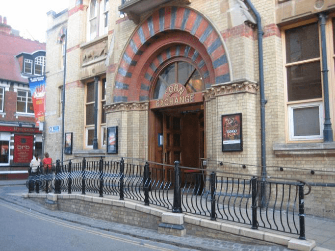
Similarly, you can check out the respective segmentation mask:
>>> dataset[index]["annotation"]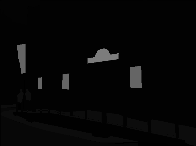
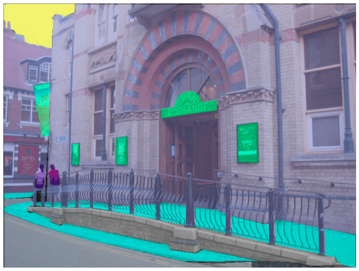
We can also add a color palette on the segmentation mask and overlay it on top of the original image to visualize the dataset:
After defining the color palette, you should be ready to visualize some overlays.
>>> import matplotlib.pyplot as plt

>>> def visualize_seg_mask(image: np.ndarray, mask: np.ndarray):
...    color_seg = np.zeros((mask.shape[0], mask.shape[1], 3), dtype=np.uint8)
...    palette = np.array(create_ade20k_label_colormap())
...    for label, color in enumerate(palette):
...        color_seg[mask == label, :] = color
...    color_seg = color_seg[..., ::-1]  # convert to BGR

...    img = np.array(image) * 0.5 + color_seg * 0.5  # plot the image with the segmentation map
...    img = img.astype(np.uint8)

...    plt.figure(figsize=(15, 10))
...    plt.imshow(img)
...    plt.axis("off")
...    plt.show()


>>> visualize_seg_mask(
...     np.array(dataset[index]["image"]),
...     np.array(dataset[index]["annotation"])
... )
Now apply some augmentations with albumentations. You’ll first resize the image and adjust its brightness.
>>> import albumentations

>>> transform = albumentations.Compose(
...     [
...         albumentations.Resize(256, 256),
...         albumentations.RandomBrightnessContrast(brightness_limit=0.3, contrast_limit=0.3, p=0.5),
...     ]
... )
Create a function to apply the transformation to the images:
>>> def transforms(examples):
...     transformed_images, transformed_masks = [], []
...
...     for image, seg_mask in zip(examples["image"], examples["annotation"]):
...         image, seg_mask = np.array(image), np.array(seg_mask)
...         transformed = transform(image=image, mask=seg_mask)
...         transformed_images.append(transformed["image"])
...         transformed_masks.append(transformed["mask"])
...
...     examples["pixel_values"] = transformed_images
...     examples["label"] = transformed_masks
...     return examples
Use the set_transform() function to apply the transformation on-the-fly to batches of the dataset to consume less disk space:
>>> dataset.set_transform(transforms)You can verify the transformation worked by indexing into the pixel_values and label of an example:
>>> image = np.array(dataset[index]["pixel_values"])
>>> mask = np.array(dataset[index]["label"])

>>> visualize_seg_mask(image, mask)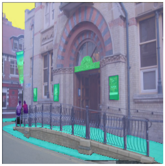
In this guide, you have used albumentations for augmenting the dataset. It’s also possible to use torchvision to apply some similar transforms.
>>> from torchvision.transforms import Resize, ColorJitter, Compose

>>> transformation_chain = Compose([
...     Resize((256, 256)),
...     ColorJitter(brightness=0.25, contrast=0.25, saturation=0.25, hue=0.1)
... ])
>>> resize = Resize((256, 256))

>>> def train_transforms(example_batch):
...     example_batch["pixel_values"] = [transformation_chain(x) for x in example_batch["image"]]
...     example_batch["label"] = [resize(x) for x in example_batch["annotation"]]
...     return example_batch

>>> dataset.set_transform(train_transforms)

>>> image = np.array(dataset[index]["pixel_values"])
>>> mask = np.array(dataset[index]["label"])

>>> visualize_seg_mask(image, mask)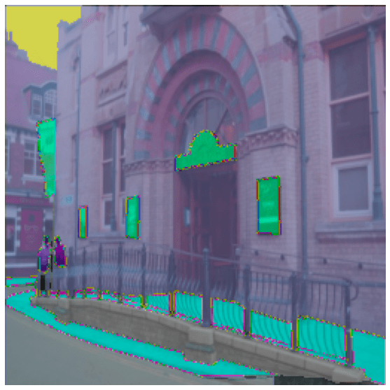
Update on GitHubNow that you know how to process a dataset for semantic segmentation, learn how to train a semantic segmentation model and use it for inference.