
questionid
stringlengths 36
36
| RA_number
int64 0
23
| RA_choice
int64 0
10
| RA_none
int64 0
9
| modulename
int64 0
24
| module
int64 0
6
| level
int64 0
3
| setnumber
int64 0
17
| questionnumber
int64 0
32
| masterContent
stringlengths 2
447k
⌀ | partContent
stringlengths 9
447k
| partposition
int64 1
11
| skill
float64 0
1
| roundedDuration
int64 0
4
| tutorial
stringlengths 2
4.74k
⌀ | workedsolution
stringlengths 2
20.4k
⌀ | total_text
stringlengths 47
447k
⌀ | text_len
int64 1
1.95k
| latex_len
int64 0
115
| latex_len_solution
int64 0
95
| latex_len_tutorial
int64 0
95
| text_len_solution
int64 0
2.89k
| text_len_tutorial
int64 0
83
| text_len_parts
int64 1
1.87k
| latex_len_parts
int64 0
108
| embeddings
int64 0
8
| questionContent
stringlengths 15
5.94k
| question_sentence_len
int64 0
47
|
|---|---|---|---|---|---|---|---|---|---|---|---|---|---|---|---|---|---|---|---|---|---|---|---|---|---|---|---|
001f060c-6b7e-4705-a37d-f740a61334a2 | 4 | 0 | 0 | 2 | 1 | 2 | 3 | 4 | Water (density $\rho _{H_{2}O}=1000\,$kg/m$^3$) flows up the slanted pipe, which is at an angle of $\theta=30^\circ\,$to the horizontal, as shown below.
  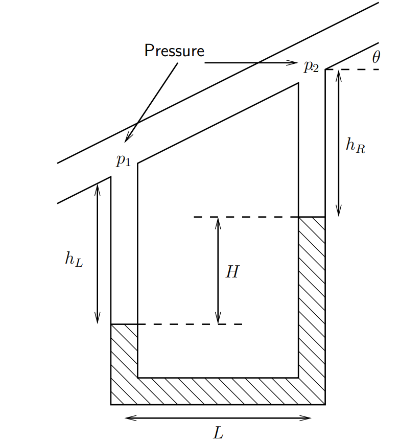
The bottom of the loop is filled with mercury (density $\rho_{Hg}=13,600\,$kg/m$^3$), which acts as a manometer, and you may assume is not flowing. The loop has width $L=5\,$cm, and in this question you should assume that $g=10\,$m/s$^2$.
(Based on P2.35 in White) 
| What would be the pressure drop $p_1 - p_2\,$if the fluid were stationary?
\nIf the height difference $H=0.1\,$cm, what is the pressure difference $p_1-p_2\,$ in the pipe? You may use the fact that from geometry we have $H+h_r-h_L=L\tan(\theta)$.
\nWhat is the difference between the values in parts 5b and 5a? Why is this extra pressure needed?
\nIf the fluid were not flowing, what would the height difference $H\,$ be?
| 4 | 0.666667 | 3 | The pressure difference would be given by $p_1-p_2=\rho gz$. Find $z$ (length of the opposite part of the triangle) by creating a triangle using $L$ and the angle $\theta$ given in the question. Substitute this and all values given back in to get a final numerical answer.
\nWe cannot simply calculate the hydrostatic pressure difference between the two points. This is because the water is flowing, meaning that the pressure is not hydrostatic. Let us define the pressure at the water--mercury interface in the left-hand arm as $p_L$, and the height of the column of water above that point as $h_L$, and let us define the column of water in the right-hand arm as $h_R$.
From the geometry, we have
$H+h_R-h_L=L\tan\theta.$
From hydrostatic balance (i.e. using the general pressure equation $p=p_0 -\rho gz$ and finding $p_0$ and substituting in) find $p_1$ and $p_2$.
***
We get $p_1=p_L-\rho_{H_2O}gh_L$ and $p_2=p_L-\rho_{Hg}gH-\rho_{H_2O}gh_R.$ Now take $p_2$ away form $p_1$ to find the pressure difference. 
***
We get $p_1-p_2=\rho_{Hg}gH+\rho_{H_2O}gh_R-\rho_{H_2O}gh_L$. Simplify to get an expression which factors out $h_R$ and $h_L$. Use the equation form the geometry to replace $h_R - h_L$
***
Substitute in values from the question to get your final numeric answer
\n\nTo understand this, suppose that the depths of mercury are $d_L$ and $d_R$ in the left-hand and right-hand columns of the manometer, respectively. Consider travelling from the bottom of the U-bend through the left-hand tube and along the slanted pipe to the point where $p_2$ is measured. We go through a depth $d_L$ of mercury and $h_{TOT}-d_L$ of water, where $h_{TOT}$ is the total height.
***
Compare that with travelling up the right-hand tube to the same point, in which case we go through a depth $d_R$ and $h_{\sf TOT}-d_R$ of mercury and water, respectively.
***
The total pressure change on the left path equals $\rho_{Hg}gd_L+\rho_{H_2O}g(h_{TOT}-d_L)$, whilst the pressure change on the right path equals $\rho_{Hg}gd_R+\rho_{H_2O}g(h_{TOT}-d_R)$. These two pressure changes must be equal, and the only way this can happen is if $d_L=d_R$. Hence $H=0$.
| The pressure difference between the two points would be given by the hydrostatic formula: $p_1-p_2=\rho gL\tan\theta=1,000\times10\times0.05\tan30^\circ=290$Pa.
\nWe cannot simply calculate the hydrostatic pressure difference between the two points. This is because the water is flowing, meaning that the pressure is not hydrostatic. Let us define the pressure at the water--mercury interface in the left-hand arm as $p_L$, and the height of the column of water above that point as $h_L$, and let us define the column of water in the right-hand arm as $h_R$.
From the geometry, we have
$H+h_R-h_L=L\tan\theta.$
Using hydrostatic balance in the left column, we have
$p_1=p_L-\rho_{H_2O}gh_L.$
The hydrostatic balance in the right-hand column gives
$p_2=p_L-\rho_{Hg}gH-\rho_{H_2O}gh_R.$
Hence
$p_1-p_2=\rho_{Hg}gH+\rho_{H_2O}gh_R-\rho_{H_2O}gh_L$
$=\rho_{Hg}gH+\rho_{H_2O}g(h_R-h_L)$
$=\rho_{Hg}gH+\rho_{H_2O}g(L\tan\theta-H)$
$=13,600\times10\times0.001+1000\times10\times(0.05\tan30^\circ-0.001)$
$=136+279=410$ Pa (2 s.f.).
\n\nIn this case the pressure is hydrostatic, which means that $H=0$.
To understand this, suppose that the depths of mercury are $d_L$ and $d_R$ in the left-hand and right-hand columns of the manometer, respectively. Consider travelling from the bottom of the U-bend through the left-hand tube and along the slanted pipe to the point where $p_2$ is measured. We go through a depth $d_L$ of mercury and $h_{TOT}-d_L$ of water, where $h_{TOT}$ is the total height. Compare that with travelling up the right-hand tube to the same point, in which case we go through a depth \$d\_R\$ and $h_{\sf TOT}-d_R$ of mercury and water, respectively. The total pressure change on the left path equals $\rho_{Hg}gd_L+\rho_{H_2O}g(h_{TOT}-d_L)$, whilst the pressure change on the right path equals $\rho_{Hg}gd_R+\rho_{H_2O}g(h_{TOT}-d_R)$. These two pressure changes must be equal, and the only way this can happen is if $d_L=d_R$. Hence $H=0$.
| Water (density $\rho _{H_{2}O}=1000\,$kg/m$^3$) flows up the slanted pipe, which is at an angle of $\theta=30^\circ\,$to the horizontal, as shown below.
  
The bottom of the loop is filled with mercury (density $\rho_{Hg}=13,600\,$kg/m$^3$), which acts as a manometer, and you may assume is not flowing. The loop has width $L=5\,$cm, and in this question you should assume that $g=10\,$m/s$^2$.
(Based on P2.35 in White) 
What would be the pressure drop $p_1 - p_2\,$if the fluid were stationary?
\nIf the height difference $H=0.1\,$cm, what is the pressure difference $p_1-p_2\,$ in the pipe? You may use the fact that from geometry we have $H+h_r-h_L=L\tan(\theta)$.
\nWhat is the difference between the values in parts 5b and 5a? Why is this extra pressure needed?
\nIf the fluid were not flowing, what would the height difference $H\,$ be?
| 145 | 13 | 25 | 25 | 270 | 32 | 70 | 5 | 1 | The bottom of the loop is filled with mercury density $\rho_{Hg}=13,600\,$kg/m$^3$, which acts as a manometer, and you may assume is not flowing. The loop has width $L=5\,$cm, and in this question you should assume that $g=10\,$m/s$^2$. Based on P2.35 in White What would be the pressure drop $p_1 - p_2\,$if the fluid were stationary? If the height difference $H=0.1\,$cm, what is the pressure difference $^3$0 in the pipe? You may use the fact that from geometry we have $^3$1. What is the difference between the values in parts 5b and 5a? Why is this extra pressure needed? If the fluid were not flowing, what would the height difference $^3$2 be? | 8 |
008875c9-9c5b-4f18-b79c-e21c3ed8e14f | 4 | 4 | 0 | 19 | 6 | 1 | 5 | 2 | **(L8)**: Use Gaussian elimination to solve the system of equations below (**Note**: these are the same equations as Q1, so you know the type of solution to expect).
***
You are asked to input the nature of the intersection of the planes. If the planes intersect at a point, input the point of intersection. If not, look at the '*Final Answer*' to check if your equation of intersection is correct.
| $$
\begin{aligned}
x+y+z&=6\, ,\\
2x+y-z&=3\, ,\\
x+y&=4\, .
\end{aligned}
$$
\n$$
\begin{aligned}
x+y+z&=6\, ,\\
2x+y-z&=3\, ,\\
4x+3y+z&=1\, .
\end{aligned}
$$
\n$$
\begin{aligned}
x+y+z&=6\, ,\\
2x+y-z&=3\, ,\\
2x+2y+2z&=12\, .
\end{aligned}
$$
\n$$
\begin{aligned}
-x+2y-2z&=1, \\
4x-y+6z&=2\, ,\\
2x+3y+2z&=4\, ,\\
\end{aligned}
$$
| 4 | 0.666667 | 3 | Before starting Gaussian Elimination, ensure you have answered *Question 1* to identify the type of solution that you will expect.
***
Set-up the augmented matrix (**section 2.8**)...
***
... Attempt to manipulate the matrix into triangular form, e.g. :
$$
\left( \begin{array}{ccc|r} a & b & c & \ d\\ 0 & e & f & g\\ 0 & 0 & h & i \end{array} \right)
$$
There are three cases that can occur (**section 2.9**, **2.10**, **2.11**)...
***
1. $h=0$ and $i=0$ (i.e., R3 is a row of zeros). In this case, you will be able to derive a line/plane of intersection. 
2. $h=0$ and $i\ne0$. This is an inconsistency, and so there are no solutions. 
3. $h\ne0$. In this case, you can solve for a point of intersection $(x,y,z)$. 
(see more information on case 1 and 3 below)...
***
... In *case 1*, to derive the line/plane equation, take the equations out of augmented matrix form, and set one variable equal to $\lambda$. Then, solve for $\lambda$. 
***
In *case 3*, manipulate the matrix into the form:
$$
\left( \begin{array}{ccc|r} 1 & 0 & 0 & \ a\\ 0 & 1 & 0 & b\\ 0 & 0 & 1 & c \end{array} \right)
$$
Now $x=a,y=b,z=c$. 
\nBefore starting Gaussian Elimination, it may help you to answer *Question 1* to identify the type of solution that you will expect.
***
Set-up the augmented matrix (**section 2.8**)...
***
... Attempt to manipulate the matrix into triangular form, e.g. :
$$
\left( \begin{array}{ccc|r} a & b & c & \ d\\ 0 & e & f & g\\ 0 & 0 & h & i \end{array} \right)
$$
There are three cases that can occur (**section 2.9**, **2.10**, **2.11**)...
***
1. $h=0$ and $i=0$ (i.e., R3 is a row of zeros). In this case, you will be able to derive a line/plane of intersection. 
2. $h=0$ and $i\ne0$. This is an inconsistency, and so there are no solutions. 
3. $h\ne0$. In this case, you can solve for a point of intersection $(x,y,z)$. 
(see more information on case 1 and 3 below)...
***
... In *case 1*, to derive the line/plane equation, take the equations out of augmented matrix form, and set one variable equal to $\lambda$. Then, solve for $\lambda$. 
***
In *case 3*, manipulate the matrix into the form:
$$
\left( \begin{array}{ccc|r} 1 & 0 & 0 & \ a\\ 0 & 1 & 0 & b\\ 0 & 0 & 1 & c \end{array} \right)
$$
Now $x=a,y=b,z=c$. 
| Refer to **section 2.8** for Gaussian elimination rules. In question 1 (a), we found that this system of equations intersects at a point. Therefore, we will attempt to re-arrange the augmented matrix into the form:
$$
\left( \begin{array}{ccc|r} 1 & 0 & 0 & \ a\\ 0 & 1 & 0 & b\\ 0 & 0 & 1 & c \end{array} \right)
$$
Setting up the augmented matrix:
***
$$
\left( \begin{array}{ccc|r} 1 & 1 & 1 & \ 6\\ 2 & 1 & -1 & 3\\ 1 & 1 & 0 & 4 \end{array} \right)
$$
***
* R2-2R1
* R3-R1
***
$$
\rightarrow\left( \begin{array}{ccc|r} 1 & 1 & 1 & \ 6\\ 0 & -1 & -3 & -9\\ 0 & 0 & -1 & -2 \end{array} \right)
$$
***
* \-R2, -R3
***
$$
\rightarrow \left(\begin{array}{ccc|r} 1 & 1 & 1 & \ 6\\ 0 & 1 & 3 & 9\\ 0 & 0 & 1 & 2 \end{array} \right)
$$
***
* R1-R3
* R2-3R3
***
$$
\rightarrow \left(\begin{array}{ccc|r} 1 & 1 & 0 & \ 4\\ 0 & 1 & 0 & 3\\ 0 & 0 & 1 & 2 \end{array} \right)
$$
***
* R1-R2
***
$$
\rightarrow \left(\begin{array}{ccc|r} 1 & 0 & 0 & \ 1\\ 0 & 1 & 0 & 3\\ 0 & 0 & 1 & 2 \end{array} \right)
$$
***
Hence the point of intersection is $x=1,y=3,z=2\rightarrow(1,3,2)$
\nRefer to **section 2.8** for Gaussian elimination rules. In question 1 (b), we found that this system of equations has **no solutions**. This can be verified using Gaussian elimination.
Setting up the augmented matrix:
***
$$
\left(\begin{array}{ c c c | c }
1 & 1 & 1 & 6\\
2 & 1 & -1 & 3\\
4 & 3 & 1 & 1
\end{array}\right)
$$
***
* R2-2R1
* R3-4R1
***
$$
\rightarrow\left(\begin{array}{ c c c | c }
1 & 1 & 1 & 6\\
0 & -1 & -3 & -9\\
0 & -1 & -3 & -23
\end{array}\right)
$$
***
* R3-R2, -R2:
***
$$
\left(\begin{array}{ c c c | c }
1 & 1 & 1 & 6\\
0 & 1 & 3 & 9\\
0 & 0 & 0 & -14
\end{array}\right)
$$
***
The bottom row is inconsistent, because $0\ne14$. Hence we have no solutions, as expected. 
\nRefer to **section 2.8** for Gaussian elimination rules. In question 1 (b), we found that this system of equations has an infinity of solutions. The goal is to find the equation of the line/plane along which these planes intersect. Setting up the augmented matrix:
***
$$
\left( \begin{array}{ccc|r} 1 & 1 & 1 & 6\\ 2 & 1 & -1 & 3\\ 2 & 2 & 2 & 12 \end{array} \right)
$$
***
* R3-2R1 (notice that R3=2R1). 
* R2-2R1
***
$$
\rightarrow \left(\begin{array}{ccc|r} 1 & 1 & 1 & 6\\ 0 & -1 & -3 & -9\\ 0 & 0 & 0 & 0 \end{array} \right)
$$
The third line is consistent, as it implies that $0=0$. Simplifying R1 and R2:
***
* R1+R2
* \-R2
***
$$
\rightarrow \left(\begin{array}{ccc|r}1 & 0 & -2 & -3\\ 0 & 1 & 3 & 9\\ 0 & 0 & 0 & 0 \end{array} \right)
$$
***
Now, exiting the augmented matrix:
***
$$
\begin{aligned}
&x-2z=-3\\
&y+3z=9
\end{aligned}
$$
Setting $z=\lambda$:
***
$$
\begin{align*}
\begin{array}{r l}
x & =-3 + 2\lambda\, ,\\
y &= 9-3\lambda ,\\
z &= \lambda\, .
\end{array} \Bigg\} \qquad
\begin{pmatrix} x \\ y \\ z \end{pmatrix} =
\begin{pmatrix} -3 \\ 9 \\ 0 \end{pmatrix} +
\lambda \begin{pmatrix} 2 \\ -3 \\ \ 1 \end{pmatrix}
\end{align*}
$$
This is the vector equation of a line; or, in Cartesian form:
***
$$
\lambda = \dfrac{x+3}{2} = \dfrac{9-y}{3} = z
$$
\nRefer to **section 2.8** for Gaussian elimination rules. In question 1 (b), we found that this system of equations has an infinity of solutions. The goal is to find the equation of the line/plane along which these planes intersect. Setting up the augmented matrix:
***
$$
\left( \begin{array}{ccc|r} -1 & 2 & -2 & 1\\ 4 & -1 & 6 & 2\\ 2 & 3 & 2 & 4 \end{array} \right)
$$
***
* R2+4R1
* R3+2R1
***
$$
\rightarrow \left( \begin{array}{ccc|r} -1 & 2 & -2 & 1\\ 0 & 7 & -2 & 6\\ 0 & 7 & -2 & 6 \end{array} \right)
$$
***
* R1-R2
* R3-R2
***
$$
\rightarrow\left( \begin{array}{ccc|r} -1 & -5 & 0 & -5\\ 0 & 7 & -2 & 6\\ 0 & 0 & 0 & 0 \end{array} \right)\rightarrow\left( \begin{array}{ccc|r} 1 & 5 & 0 & 5\\ 0 & 7 & -2 & 6\\ 0 & 0 & 0 & 0 \end{array} \right)
$$
In the final stage, we took -R1. The third line is consistent, as it implies that $0=0$. 
***
Exiting the augmented matrix:
***
$$
\begin{aligned}
&x+5y=5\\
&7y-2z=6
\end{aligned}
$$
Setting $y=\lambda$:
***
$$
\begin{align*}
\begin{array}{r l}
x & = 5 - 5 \lambda\, ,\\
y &= \lambda ,\\
z &= -3 + \tfrac{7}{2} \lambda\,
\end{array} \Bigg\} \qquad
\begin{pmatrix} x \\ y \\ z \end{pmatrix} =
\begin{pmatrix} 5 \\ 9 \\ -3 \end{pmatrix} +
\lambda \begin{pmatrix} -5 \\ 1 \\ \ \tfrac{7}{2} \end{pmatrix}
\end{align*}
$$
This is the vector equation of a line; or, in Cartesian form:
***
$$
\lambda = \dfrac{5-x}{5} = y = \dfrac{2z+6}{7}
$$
| **(L8)**: Use Gaussian elimination to solve the system of equations below (**Note**: these are the same equations as Q1, so you know the type of solution to expect).
***
You are asked to input the nature of the intersection of the planes. If the planes intersect at a point, input the point of intersection. If not, look at the '*Final Answer*' to check if your equation of intersection is correct.
$$
\begin{aligned}
x+y+z&=6\, ,\\
2x+y-z&=3\, ,\\
x+y&=4\, .
\end{aligned}
$$
\n$$
\begin{aligned}
x+y+z&=6\, ,\\
2x+y-z&=3\, ,\\
4x+3y+z&=1\, .
\end{aligned}
$$
\n$$
\begin{aligned}
x+y+z&=6\, ,\\
2x+y-z&=3\, ,\\
2x+2y+2z&=12\, .
\end{aligned}
$$
\n$$
\begin{aligned}
-x+2y-2z&=1, \\
4x-y+6z&=2\, ,\\
2x+3y+2z&=4\, ,\\
\end{aligned}
$$
| 77 | 4 | 27 | 27 | 350 | 44 | 7 | 4 | 0 | L8: Use Gaussian elimination to solve the system of equations below Note: these are the same equations as Q1, so you know the type of solution to expect. \end{aligned} $ $ \begin{aligned} x+y+z&=6\, ,\\ 2x+y-z&=3\, ,\\ 4x+3y+z&=1\, . \end{aligned} $ $ \begin{aligned} x+y+z&=6\, ,\\ 2x+y-z&=3\, ,\\ 2x+2y+2z&=12\, . \end{aligned} $ $ \begin{aligned} -x+2y-2z&=1, \\ 4x-y+6z&=2\, ,\\ 2x+3y+2z&=4\, ,\\ \end{aligned} $ | 4 |
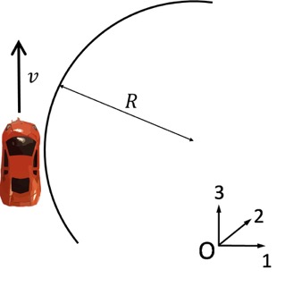
012cc4b4-bb47-4ac4-a702-370084cef4cd | 1 | 2 | 0 | 13 | 4 | 2 | 5 | 2 | An experimental vehicle is fitted with a gyroscope to counteract completely the tendency of the vehicle to tip when rounding a bend.
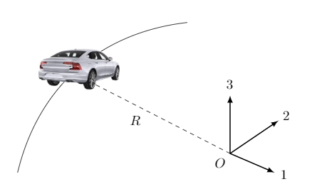
The gyroscope rotor is mounted on a horizontal shaft fixed across the vehicle frame, parallel with the rear axle and has a mass moment of inertia $I = 3000~\mathrm{kgm^2}$ about its spin axis. The vehicle has a total mass $m = 1200~\mathrm{kg}$ and its centre of mass is at a height $h = 0.8~\mathrm{m}$ above the road surface. The mass of the wheels may be ignored. The situation is modelled as follows:
In the diagram, the coordinate system is at the centre of the car's circular motion. The car's velocity is in the direction labelled 2, direction 1 is perpendicular to the car's velocity and directed away from the car's position, whilst 3 is the upward normal to the road surface.
| Find the angular velocity $\Omega$ that the gyroscope rotor should spin at if the car is travelling with velocity $v = 15~\mathrm{m/s}$.
\nIn which direction should the gyroscope spin?
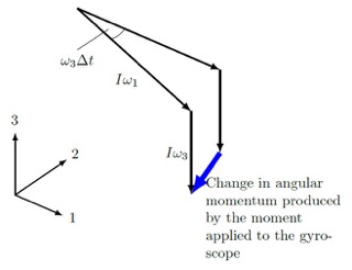
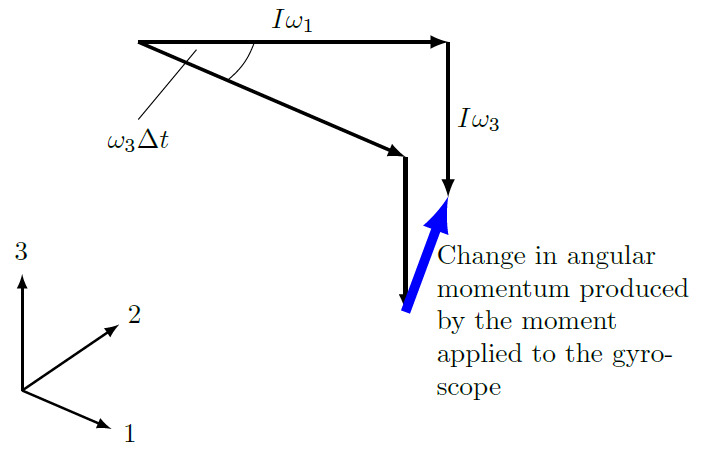
\nObserve the two diagrams below:
### **Diagram A**
### **Diagram B**
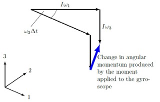
Which diagram shows the correct change in angular momentum caused by the gyroscope?
| 3 | 0.666667 | 4 | Draw the car rounding a bend and introduce a suitable system for your vector conventions. The question may seem complicated but the solution is fairly straight forward.
***
Relate the car speed $v$ and the radius of the bend to its angular momentum around the centre of the bend.
***
You’ll then need to think of an expression describing the moment imposed on the car through the wheels due to the centripetal force taking into account $h$, the height of the centre of mass of the car off the ground – this is the moment you need to counteract with the gyro!
***
Combining these two expressions and Equation 5.1 from your notes will give you an expression of the required angular velocity of the gyro, taking the angular velocity of precession as the angular velocity of the whole car around the bend.
\nThe direction of spin required can be deducted using your vector diagram of the change in angular momentum once again, making use of the right hand rule one last time.
\nSee worked solutions in part a
| 
***
Centripetal moment applied to the car:
$$
M=\cfrac{{mv}^2h}{R}~~\mathrm{(Equation~1)}
$$
***
Where:
$$
v=\omega_3R~~\mathrm{(Equation~2)}
$$
***
Substituting Equation 2 into Equation 1:
$$
M=mv\omega_3h~~\mathrm{(Equation~3)}
$$
***
Moment applied to the gyroscope:
$$
M=I\omega_3\omega_1~~\mathrm{(Equation~4)}
$$
***
If the gyroscope spins in the opposite direction to the wheels, the gyroscope vector diagram is shown below:
***
Equating the moments from Equations 3 and 4:
$$
M=mv\omega_3h=I\omega_3\omega_1
$$
***
Hence the angular velocity of the rotor is:
$$
\omega_1=\cfrac{mvh}{I}
$$
***
Substituting the values of the parameters gives:
$$
\omega_1=\cfrac{1200\times15\times0.8}{3000}
$$
$$
\omega_1=4.8~\mathrm{rad/s}
$$
(In a direction opposite to the road wheels)
\n\n | An experimental vehicle is fitted with a gyroscope to counteract completely the tendency of the vehicle to tip when rounding a bend.

The gyroscope rotor is mounted on a horizontal shaft fixed across the vehicle frame, parallel with the rear axle and has a mass moment of inertia $I = 3000~\mathrm{kgm^2}$ about its spin axis. The vehicle has a total mass $m = 1200~\mathrm{kg}$ and its centre of mass is at a height $h = 0.8~\mathrm{m}$ above the road surface. The mass of the wheels may be ignored. The situation is modelled as follows:
In the diagram, the coordinate system is at the centre of the car's circular motion. The car's velocity is in the direction labelled 2, direction 1 is perpendicular to the car's velocity and directed away from the car's position, whilst 3 is the upward normal to the road surface.
Find the angular velocity $\Omega$ that the gyroscope rotor should spin at if the car is travelling with velocity $v = 15~\mathrm{m/s}$.
\nIn which direction should the gyroscope spin?
\nObserve the two diagrams below:
### **Diagram A**

### **Diagram B**

Which diagram shows the correct change in angular momentum caused by the gyroscope?
| 190 | 5 | 8 | 8 | 86 | 2 | 53 | 2 | 3 | The situation is modelled as follows: In the diagram, the coordinate system is at the centre of the car's circular motion. Find the angular velocity $\Omega$ that the gyroscope rotor should spin at if the car is travelling with velocity $v = 15~\mathrm{m/s}$. In which direction should the gyroscope spin? Observe the two diagrams below: ### Diagram A ### Diagram B Which diagram shows the correct change in angular momentum caused by the gyroscope? | 4 |
01e1b7d0-d39c-4cdf-8200-05e95de00232 | 4 | 0 | 0 | 6 | 4 | 1 | 2 | 1 | As part of another design project, you are tasked with verifying whether a certain engine is suitable for driving the wheels of a lawn mower. You need to check that the engine will have a suitable cylinder capacity to generate the required 3kW of power at its minimum operating speed.
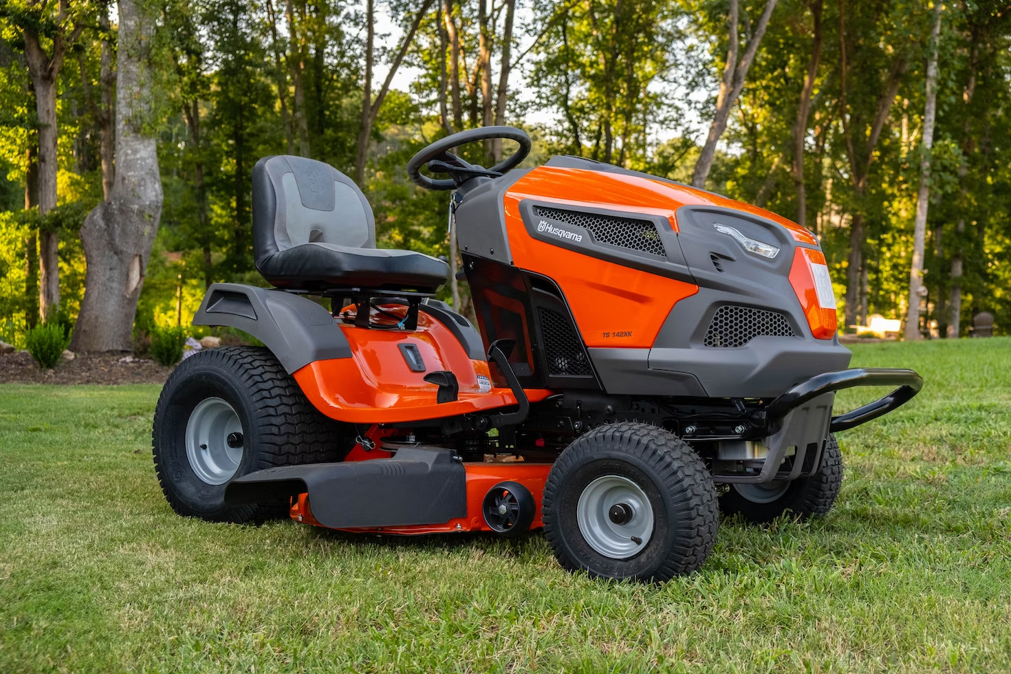
| First, given that the lawnmower is rated for speeds between 1 and 5 m/s, you need to determine the range of the engine rpm if the lawn mower wheels are 0.4m in diameter and the following drive transmission is used: (you may assume no change in rotational speed other than from the drive transmission below)
| Stage | First Transmission Component | Second Transmission Component |
| :---- | :--------------------------- | :---------------------------- |
| 1 | 14 tooth sprocket | 24 tooth sprocket |
| 2 | 30mm diameter pulley | 70mm diameter pulley |
| 3 | 10 tooth gear | 26 tooth gear |
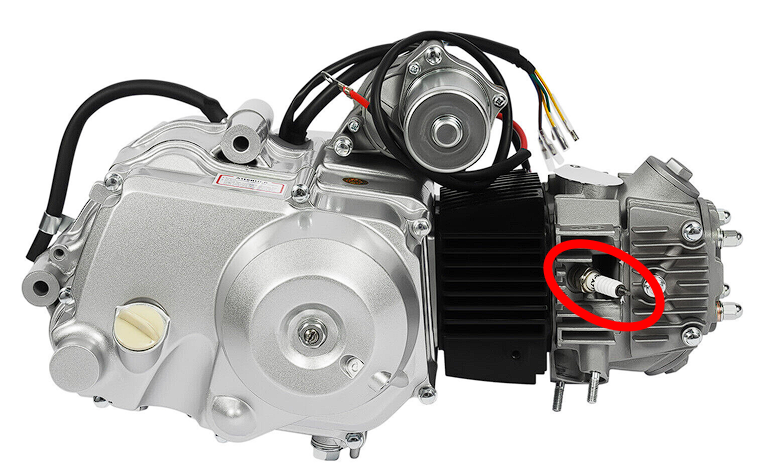
\nThe engine you need to confirm the performance of is shown below:
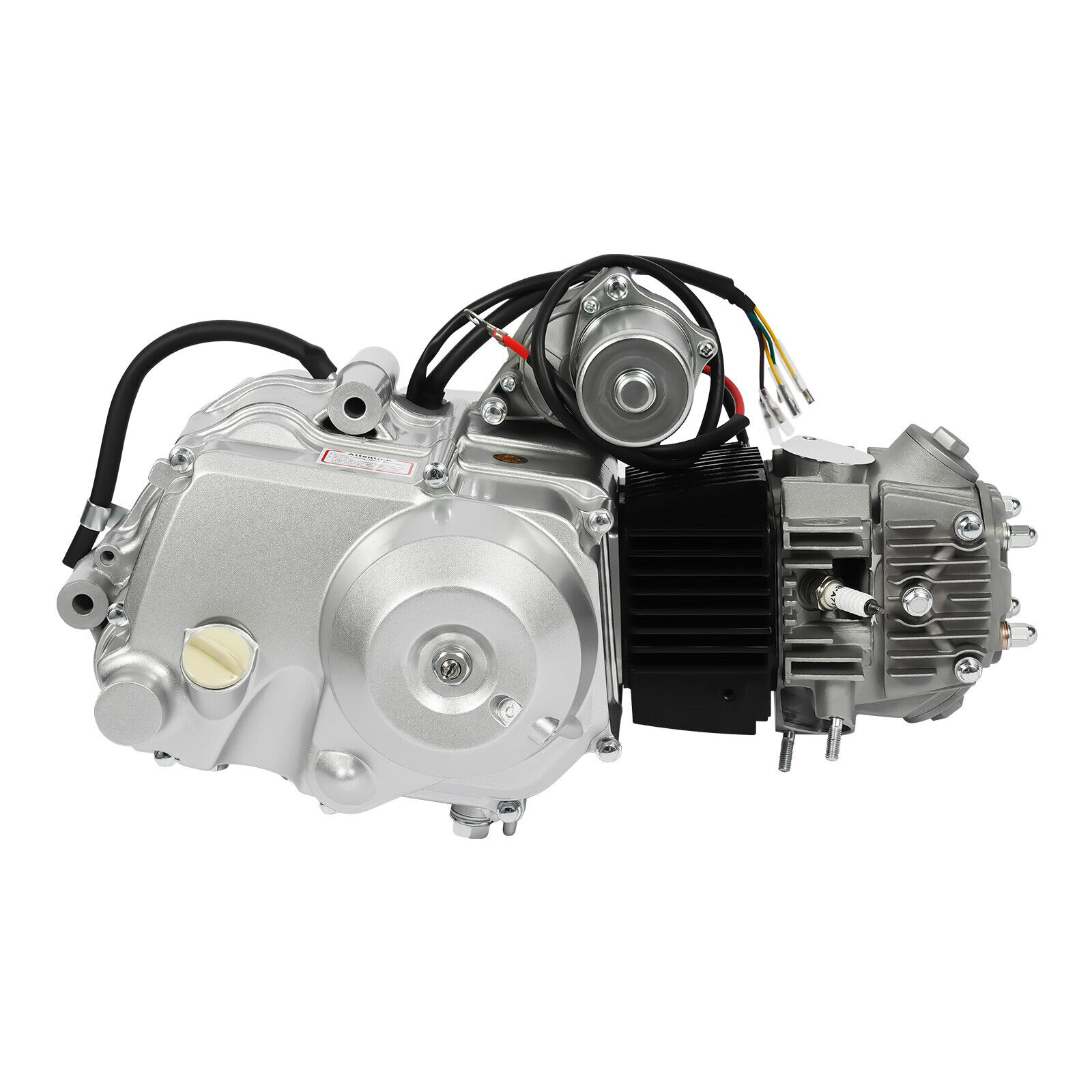Given that the temperature and pressure at stages 1, 2, 3 and 4 are as shown in the table below, determine the specific net work of the engine.
| Stage | Temperature (K) | Pressure (bar) |
| :---- | :-------------- | :------------- |
| 1 | 298 | 1.013 |
| 2 | | |
| 3 | | |
| 4 | | |
\nDetermine the minimum required cylinder capacity to ensure a minimum of 3kW is supplied at all engine speeds.
| 3 | 0.666667 | 3 | \n\nRefer to your thermodynamics problem sheets.
| \nThe first step to this question is to use the picture of the engine to determine what type of engine it is. This engine is clearly a petrol engine as you can see a spark plug in the picture.
***
Next, you need to use the SFEE to complete calculations for each process.
\n | As part of another design project, you are tasked with verifying whether a certain engine is suitable for driving the wheels of a lawn mower. You need to check that the engine will have a suitable cylinder capacity to generate the required 3kW of power at its minimum operating speed.

First, given that the lawnmower is rated for speeds between 1 and 5 m/s, you need to determine the range of the engine rpm if the lawn mower wheels are 0.4m in diameter and the following drive transmission is used: (you may assume no change in rotational speed other than from the drive transmission below)
| Stage | First Transmission Component | Second Transmission Component |
| :---- | :--------------------------- | :---------------------------- |
| 1 | 14 tooth sprocket | 24 tooth sprocket |
| 2 | 30mm diameter pulley | 70mm diameter pulley |
| 3 | 10 tooth gear | 26 tooth gear |
\nThe engine you need to confirm the performance of is shown below:
Given that the temperature and pressure at stages 1, 2, 3 and 4 are as shown in the table below, determine the specific net work of the engine.
| Stage | Temperature (K) | Pressure (bar) |
| :---- | :-------------- | :------------- |
| 1 | 298 | 1.013 |
| 2 | | |
| 3 | | |
| 4 | | |
\nDetermine the minimum required cylinder capacity to ensure a minimum of 3kW is supplied at all engine speeds.
| 253 | 0 | 0 | 0 | 56 | 0 | 202 | 0 | 1 | As part of another design project, you are tasked with verifying whether a certain engine is suitable for driving the wheels of a lawn mower. First, given that the lawnmower is rated for speeds between 1 and 5 m/s, you need to determine the range of the engine rpm if the lawn mower wheels are 0.4m in diameter and the following drive transmission is used: you may assume no change in rotational speed other than from the drive transmission below table Determine the minimum required cylinder capacity to ensure a minimum of 3kW is supplied at all engine speeds. | 2 |
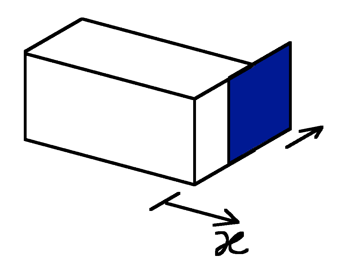
02c18d44-dd40-467d-b0e5-1ad57dc32713 | 0 | 0 | 2 | 24 | 6 | 1 | 0 | 14 | In ordinary derivatives a function $y(x)$ implicitly defines $x=x(y)$ and their derivatives obey:
$$
\frac{dx}{dy} = \frac{1}{\left(\dfrac{dy}{dx}\right)}
$$
(check e.g. for $y=x^2$). In higher dimensions a similar relation holds, but it is important to keep track of which variable is being kept constant. The correct relation is
$$
\left( \frac{\partial y}{\partial x}\right)_{z} = \frac{1}{ \left(\dfrac{\partial x}{\partial y}\right)_{z}}
$$
but e.g.
$$
\left( \frac{\partial y}{\partial x}\right)_{z} \neq \frac{1}{ \left(\dfrac{\partial x}{\partial y}\right)_{r}}
$$
The reciprocal rule only holds if the same variable is being kept constant on both sides of the equation.
|  Confirm the above for $z=x^2-y^2$, $r=\sqrt{x^2+y^2}$ by calculating $\left(\frac{\partial y}{\partial x}\right)_{z}$, $\left(\frac{\partial x}{\partial y}\right)_{z}$, $\left(\frac{\partial y}{\partial x}\right)_{r}$, $\left(\frac{\partial x}{\partial y}\right)_{r}$. 
\nFor $z=x^2-y^2$ confirm the cyclic rule for partial derivatives
$$
\left( \frac{\partial y}{\partial x}\right)_{z}\left( \frac{\partial x}{\partial z}\right)_{y}\left( \frac{\partial z}{\partial y}\right)_{x} = -1
$$
| 2 | 0.666667 | 2 | Start by finding the partial derivatives holding $z$ constant...
***
Re-arrange $z=z(x,y)$ into the form $y=y(x,z)$. Then, find $\partial y/\partial x$ holding $z$ constant. Repeat for $x=x(y,z)$. Does the reciprocal rule hold?
***
Repeat the above process but instead holding $r$ constant. Again, does the reciprocal rule hold?
***
Does the reciprocal rule hold for partial derivatives where different variables are held constant?
\nYou have already found $(\partial y/\partial x)_z$ in part (a). Express this in terms of $x$ and $y$.
***
Re-arrange for $x=x(y,z)$ and find $(\partial x/\partial z)_y$. Can you express this in terms of $x$ and $y$? Repeat for $z=z(x,y)$. 
***
Multiply the results together. Do they equal $-1$?
| Starting with the two partial derivatives where we hold $z$ constant:
***
$$
y(x,z) = (x^2-z)^{1/2}
$$
***
Using the chain rule and holding $z$ constant:
$$
\left(\dfrac{\partial y}{\partial x}\right)_z = \frac{x}{(x^2-z)^{1/2}} = \frac{x}{y}
$$
***
$$
x(y,z)=(y^2+z)^{1/2}
$$
***
$$
\therefore\left(\dfrac{\partial x}{\partial y}\right)_z = \frac{y}{(y^2+z)^{1/2}} = \frac{y}{x}
$$
This verifies that:
$$
\left( \frac{\partial y}{\partial x}\right)_{z} = \frac{1}{ \left(\dfrac{\partial x}{\partial y}\right)_{z}}
$$
Now, for $r$:
***
$$
y(x,r) = (r^2-x^2)^{1/2}
$$
***
Using the chain rule and holding $r$ constant:
$$
\left(\dfrac{\partial y}{\partial x}\right)_r = -\frac{x}{(r^2-x^2)^{1/2}}=-\frac{x}{y}
$$
***
$$
x(y,r)=(r^2-y^2)^{1/2}
$$
***
$$
\therefore\left(\frac{\partial x}{\partial y}\right)_r = -\frac{y}{(r^2-y^2)^{1/2}} = -\frac{y}{x}
$$
This verifies that:
$$
\left( \frac{\partial y}{\partial x}\right)_{z} = \frac{1}{ \left(\dfrac{\partial x}{\partial y}\right)_{z}}
$$
This also verifies that:
$$
\left( \frac{\partial y}{\partial x}\right)_{z} \neq \frac{1}{ \left(\dfrac{\partial x}{\partial y}\right)_{r}}
$$
\nFrom part (a), 
$$
\left(\dfrac{\partial y}{\partial x}\right)_z = \frac{2x}{(x^2-z)^{1/2}} = \frac{x}{y}
$$
Now, to find the other partial derivatives: re-arranging for $x=x(y,z)$,
***
$$
x=(y^2+z)^{1/2}
$$
Partially differentiating with respect to $z$ and holding $y$ constant:
***
$$
\left(\frac{\partial x}{\partial z}\right)_y = \frac{1}{2(y^2+z)^{1/2}} = \frac{1}{2x}
$$
***
Finally, partially differentiating $z=z(x,y)$ with respect to $y$ and holding $x$ constant:
***
$$
\left(\frac{\partial z}{\partial y}\right)_x = -2y
$$
Multiplying each partial derivative together:
***
$$
\left( \frac{\partial y}{\partial x}\right)_{z}\left( \frac{\partial x}{\partial z}\right)_{y}\left( \frac{\partial z}{\partial y}\right)_{x} = \frac{x}{y}\frac{1}{2x}(-2y)= -1
$$
| In ordinary derivatives a function $y(x)$ implicitly defines $x=x(y)$ and their derivatives obey:
$$
\frac{dx}{dy} = \frac{1}{\left(\dfrac{dy}{dx}\right)}
$$
(check e.g. for $y=x^2$). In higher dimensions a similar relation holds, but it is important to keep track of which variable is being kept constant. The correct relation is
$$
\left( \frac{\partial y}{\partial x}\right)_{z} = \frac{1}{ \left(\dfrac{\partial x}{\partial y}\right)_{z}}
$$
but e.g.
$$
\left( \frac{\partial y}{\partial x}\right)_{z} \neq \frac{1}{ \left(\dfrac{\partial x}{\partial y}\right)_{r}}
$$
The reciprocal rule only holds if the same variable is being kept constant on both sides of the equation.
 Confirm the above for $z=x^2-y^2$, $r=\sqrt{x^2+y^2}$ by calculating $\left(\frac{\partial y}{\partial x}\right)_{z}$, $\left(\frac{\partial x}{\partial y}\right)_{z}$, $\left(\frac{\partial y}{\partial x}\right)_{r}$, $\left(\frac{\partial x}{\partial y}\right)_{r}$. 
\nFor $z=x^2-y^2$ confirm the cyclic rule for partial derivatives
$$
\left( \frac{\partial y}{\partial x}\right)_{z}\left( \frac{\partial x}{\partial z}\right)_{y}\left( \frac{\partial z}{\partial y}\right)_{x} = -1
$$
| 94 | 14 | 26 | 26 | 111 | 16 | 27 | 8 | 0 | Confirm the above for $z=x^2-y^2$, $r=\sqrt{x^2+y^2}$ by calculating $\left(\frac{\partial y}{\partial x}\right)_{z}$, $\left(\frac{\partial x}{\partial y}\right)_{z}$, $x=x(y)$0, $x=x(y)$1. | 1 |
0315f302-37e4-420c-89aa-1674824e3cf5 | 4 | 0 | 0 | 15 | 5 | 0 | 3 | 2 | The acid dissociation constant, $K_{a}$ , is a measure of the strength of an acid ($\mathrm{HA}$), and is defined as the equilibrium constant for the reaction:
$$
\text{HA} \rightleftharpoons \text{H}^{+}+\text{A}^{-}
$$
It has a value of:
$$
K_{a}=\frac{[H^+][A^-]}{[HA]}
$$
To create a buffer solution, we can mix together solutions of a weak acid and its conjugate base (usually supplied using a salt of the weak acid). To calculate the ratio of acid to base needed for a buffer of a particular $pH$, we use the Henderson-Hasselbalch equation, which you are now going to derive.
| Rearrange the first equation to give an expression for $[H^+]$ in terms of $K_a$, $[A^-]$ and $[HA]$
\nTake the base-10 logarithm of this equation, and simplify it, so the right hand side contains one term in $K_{a}$ and a second in $[HA]$ and $[A^-]$ . Enter $\log_{10}(x)$ as 'log10(x)'.
\nUsing the definitions of $pH$ and $pK_a$ shown below, write a equation that gives $pH$ in terms of $pK_a$ and the ratio of **acid to base**, $\frac{[HA]}{[A^{-}]}$.
$$
pK_{a}=-\log_{10}K_{a}
$$
$$
pH=-\log_{10}[H^+]
$$
\nUsing your knowledge of how logs work, give an equation for the $pH$ in terms of $pK_a$ and the ratio of **base to acid**, $\frac{[A^-]}{[HA]}$.
This *is* the Henderson-Hasselbalch equation.
| 4 | 1 | 2 | \n\n\n | $$
[H^+]=\frac{K_{a} \cdot [HA]}{[A^{-}]}
$$
\n$$
\log_{10}[H^+]=\log_{10}(\frac{K_a[HA]}{[A^-]})=\log_{10} K_a+\log_{10}(\frac{[HA]}{[A^{-}]})
$$
\nFrom the previous part:
$$
\log_{10} [H^+]=\log_{10}(\frac{K_a[HA]}{[A^-]})=\log_{10} K_a+\log_{10}(\frac{[HA]}{[A^{-}]})
$$
Multiply through by $-1$:
$$
-\log_{10} [H^+]=-\log_{10}K_a-\log_{10}(\frac{[HA]}{[A^-]})
$$
Identify the two terms as $pH$ and $pK_a$:
$$
pH=pK_a-\log_{10}(\fracpH=pK_a-\log_{10}(\frac{[HA]}{[A^-]}){[HA]}{[A^-]})
$$
\nFrom the previous part:
$$
pH=pK_a-\log_{10}(\frac{[HA]}{[A^-]})
$$
Using the identity $\log(\frac{x}{y})=-\log(\frac{y}{x})$
$$
pH=pK_a+\log_{10}\frac{[A^-]}{[HA]}
$$
| The acid dissociation constant, $K_{a}$ , is a measure of the strength of an acid ($\mathrm{HA}$), and is defined as the equilibrium constant for the reaction:
$$
\text{HA} \rightleftharpoons \text{H}^{+}+\text{A}^{-}
$$
It has a value of:
$$
K_{a}=\frac{[H^+][A^-]}{[HA]}
$$
To create a buffer solution, we can mix together solutions of a weak acid and its conjugate base (usually supplied using a salt of the weak acid). To calculate the ratio of acid to base needed for a buffer of a particular $pH$, we use the Henderson-Hasselbalch equation, which you are now going to derive.
Rearrange the first equation to give an expression for $[H^+]$ in terms of $K_a$, $[A^-]$ and $[HA]$
\nTake the base-10 logarithm of this equation, and simplify it, so the right hand side contains one term in $K_{a}$ and a second in $[HA]$ and $[A^-]$ . Enter $\log_{10}(x)$ as 'log10(x)'.
\nUsing the definitions of $pH$ and $pK_a$ shown below, write a equation that gives $pH$ in terms of $pK_a$ and the ratio of **acid to base**, $\frac{[HA]}{[A^{-}]}$.
$$
pK_{a}=-\log_{10}K_{a}
$$
$$
pH=-\log_{10}[H^+]
$$
\nUsing your knowledge of how logs work, give an equation for the $pH$ in terms of $pK_a$ and the ratio of **base to acid**, $\frac{[A^-]}{[HA]}$.
This *is* the Henderson-Hasselbalch equation.
| 202 | 23 | 11 | 11 | 34 | 0 | 111 | 18 | 0 | The acid dissociation constant, $K_{a}$ , is a measure of the strength of an acid $\mathrm{HA}$, and is defined as the equilibrium constant for the reaction: $ \text{HA} \rightleftharpoons \text{H}^{+}+\text{A}^{-} $ It has a value of: $ K_{a}=\frac{[H^+][A^-]}{[HA]} $ To create a buffer solution, we can mix together solutions of a weak acid and its conjugate base usually supplied using a salt of the weak acid. To calculate the ratio of acid to base needed for a buffer of a particular $pH$, we use the Henderson-Hasselbalch equation, which you are now going to derive. Rearrange the first equation to give an expression for $[H^+]$ in terms of $K_a$, $[A^-]$ and $[HA]$ Take the base-10 logarithm of this equation, and simplify it, so the right hand side contains one term in $K_{a}$ and a second in $[HA]$ and $[A^-]$ . Enter $\mathrm{HA}$2 as 'log10x'. Using the definitions of $pH$ and $\mathrm{HA}$4 shown below, write a equation that gives $pH$ in terms of $\mathrm{HA}$4 and the ratio of acid to base, $\mathrm{HA}$7. $\mathrm{HA}$8 $\mathrm{HA}$9 Using your knowledge of how logs work, give an equation for the $pH$ in terms of $\mathrm{HA}$4 and the ratio of base to acid, $ \text{HA} \rightleftharpoons \text{H}^{+}+\text{A}^{-} $2. | 6 |
03568619-d5de-4cc4-bbca-ed5fca655d1a | 0 | 0 | 2 | 4 | 3 | 3 | 1 | 11 | An engine was left running in a large unventilated garage, resulting in a steady-state concentration of carbon monoxide, $C_{0}=24\ \mathrm{mg/m^{3}}$. At $t=0$ the engine is turned off and a large garage door is opened. Under the assumption that buoyancy effects are negligible and that the release can be regarded one-dimensional, plot the concentration profile after one minute under the different conditions that follow.
| Assuming that there is only molecular diffusion: $D = 0.202\ \mathrm{cm^{2}/s}$.
\nAssuming the flow is turbulent: $D = 10^4\ \mathrm{cm^{2}/s}$.
| 2 | 1 | 3 | \n | Given that the vertical and lateral extent of the garage door is large, the release may be treated as being one-dimensional. We also assume that the garage has infinite length and has an opening at $x=0$, which means that the initial condition of the concentration is given by
$$
C(x,t=0)=
\begin{cases}
C_{0}&\ \ \mathrm{if}\ x\leq 0\\
0&\ \ \mathrm{if}\ x> 0,
\end{cases}
$$
and we can use the solution derived in the previous question,
$$
C(x, t) = \dfrac{C_0}{2}\mathrm{erfc}\left(\dfrac{x}{\sqrt{2} \sigma}\right).
$$
***
This solution is shown in the figure below. It should be noted that the error function is not available on the calculators you have available during the exam, so you will not be expected to evaluate this expression numerically under those conditions. Evaluation here should be done with MATLAB.
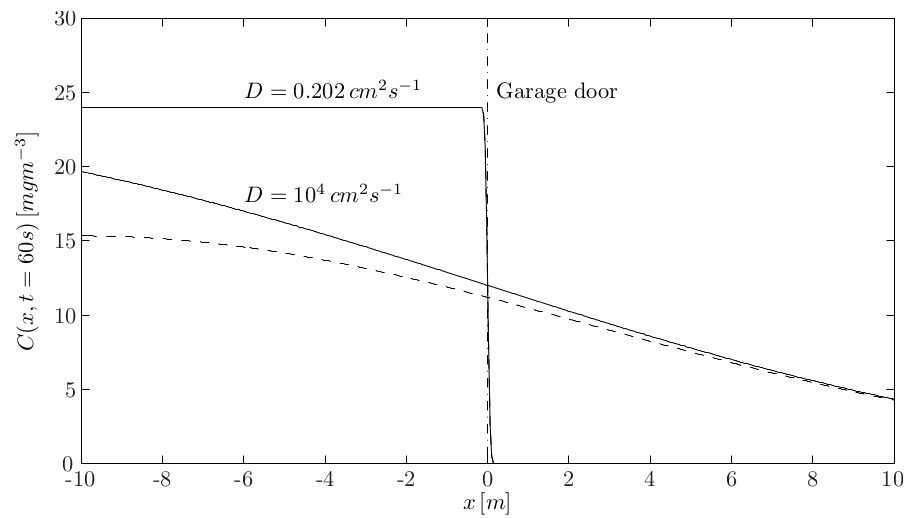
*Concentration $C\ \mathrm{[mg/m^3]}$ at $t = 60\ \mathrm{s}$ as a function of $x$; infinite garage length ($\text{---}$) and finite $(L=10\ \mathrm{m})$ garage length ($-\,-\,-$).*
\nGiven that the vertical and lateral extent of the garage door is large, the release may be treated as being one-dimensional. We also assume that the garage has infinite length and has an opening at $x=0$, which means that the initial condition of the concentration is given by
$$
C(x,t=0)=
\begin{cases}
C_{0}&\ \ \mathrm{if}\ x\leq 0\\
0&\ \ \mathrm{if}\ x> 0,
\end{cases}
$$
and we can use the solution derived in the previous question
$$
C(x, t) = \dfrac{C_0}{2}\mathrm{erfc}\left(\dfrac{x}{\sqrt{2} \sigma}\right).
$$
***
This solution is shown in the figure below. It should be noted that the error function is not available on the calculators you have available during the exam, so you will not be expected to evaluate this expression numerically under those conditions. Evaluation here should be done with MATLAB.

*Concentration $C\ \mathrm{[mg/m^3]}$ at $t = 60\ \mathrm{s}$ as a function of $x$; infinite garage length ($\text{---}$) and finite $(L=10\ \mathrm{m})$ garage length ($-\,-\,-$).*
| An engine was left running in a large unventilated garage, resulting in a steady-state concentration of carbon monoxide, $C_{0}=24\ \mathrm{mg/m^{3}}$. At $t=0$ the engine is turned off and a large garage door is opened. Under the assumption that buoyancy effects are negligible and that the release can be regarded one-dimensional, plot the concentration profile after one minute under the different conditions that follow.

Assuming that there is only molecular diffusion: $D = 0.202\ \mathrm{cm^{2}/s}$.
\nAssuming the flow is turbulent: $D = 10^4\ \mathrm{cm^{2}/s}$.
| 80 | 4 | 3 | 3 | 151 | 0 | 16 | 2 | 1 | Under the assumption that buoyancy effects are negligible and that the release can be regarded one-dimensional, plot the concentration profile after one minute under the different conditions that follow. Assuming that there is only molecular diffusion: $D = 0.202\ \mathrm{cm^{2}/s}$. Assuming the flow is turbulent: $D = 10^4\ \mathrm{cm^{2}/s}$. | 3 |
037b6b33-24e8-4efa-a376-2e2d9e5261a7 | 0 | 0 | 1 | 9 | 4 | 2 | 4 | 0 | The most readily available resistor values are the ‘E12 series’: $1, 1.2, 1.5, 1.8, 2.2, 2.7, 3.3, 3.9, 4.7, 5.6, 6.8, 8.2$ and $10~\Omega$ and factors of $10$ larger or smaller (e.g. $180~ \Omega$, $18 ~\mathrm{k}\Omega$, etc.).
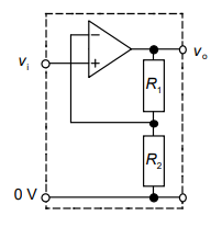
| Design a non-inverting amplifier with a gain of $263$, using fixed E12 resistors. A deviation of $\pm 1\%$ of the nominal gain is acceptable. Remember that resistors can be connected in parallel.
| 1 | 0.333333 | 1 | null | A non-inverting op-amp stage appears as follows:
  
***
For a non-inverting op-amp, the gain can be calculated as follows:
  
$A_\mathrm{v} = \frac{R_1+R_2}{R_2}$
***
This question requires a bit of trial and error. However, this can be done methodically:
***
Choose one resistor value and plug it into the above equation, along with the gain to calculate $R_2$.
***
If $R_2$ is not equal to any of the E12 resistor values, check if there is a series or parallel combination of resistors that would lead to this value.
***
Note that if there is a resistor combination that gives a gain within $1%$ of the nominal value, it is still acceptable.
| The most readily available resistor values are the ‘E12 series’: $1, 1.2, 1.5, 1.8, 2.2, 2.7, 3.3, 3.9, 4.7, 5.6, 6.8, 8.2$ and $10~\Omega$ and factors of $10$ larger or smaller (e.g. $180~ \Omega$, $18 ~\mathrm{k}\Omega$, etc.).
Design a non-inverting amplifier with a gain of $263$, using fixed E12 resistors. A deviation of $\pm 1\%$ of the nominal gain is acceptable. Remember that resistors can be connected in parallel.
| 58 | 7 | 4 | 4 | 112 | 0 | 32 | 2 | 0 | $180~ \Omega$, $18 ~\mathrm{k}\Omega$, etc.. Design a non-inverting amplifier with a gain of $263$, using fixed E12 resistors. Remember that resistors can be connected in parallel. | 2 |
03baff5d-e329-4336-8cd5-a97e93fc94a9 | 2 | 0 | 0 | 11 | 4 | 2 | 5 | 1 | At the inlet to a compressor stage, the absolute flow velocity is measured to be $250 ~\mathrm{m/s}$ at an angle of $17^{\circ}$ to the axis. 
| If the blade speed is $350 ~\mathrm{m/s}$, calculate the velocity and flow angle relative to the rotor blades.
| 1 | 0.333333 | 2 | null | Draw a velocity triangle, for which:
***
$C_2 = 250~\mathrm{m/s}$
  
$\alpha = 17^{\circ}$
  
$U = 350~\mathrm{m/s}$
***
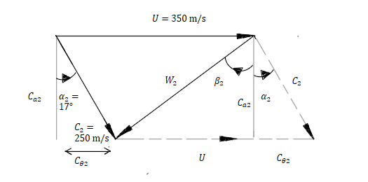
where the triangle with the dotted lines is in the same orientation as the one in the notes.
***
To find the relative velocity, $W_2$, add up the absolute and blade velocity vectors nose-to-tail:
***
$\bar{W}_2 = \bar{C}_2-\bar{U}$
***
The axial and tangential components of the absolute and blade velocities need to be calculated:
***
Absolute velocity:
***
Axial: 
  
$C_\mathrm{a2} = 250\mathrm{cos}(17)$
  
$U_\mathrm{a} =0$
***
Tangential:
  
$C_{\theta2} = 250\mathrm{sin}(17)$
  
$U_\theta = U = 350~\mathrm{m/s}$
***
Adding up the axial and tangential components and taking the magnitude:
  
$W_2 = \sqrt{(250\mathrm{cos}(17)-0)^2 + (250\mathrm{sin}(17)-350)^2} = 365.8~\mathrm{m/s}$ 
***
Calculate $\beta_2$:
  
$\beta_2 = \mathrm{cos}^{-1}(\frac{C_\mathrm{a2}}{W_2})$
***
Substituting in numbers:
  
$\beta_2 = \mathrm{cos}^{-1}(\frac{250\mathrm{cos}(17)}{365.8}) = -49.2^{\circ}$
  
Note that the angle is negative as it is measured anticlockwise from the axis $C_\mathrm{a}$.
| At the inlet to a compressor stage, the absolute flow velocity is measured to be $250 ~\mathrm{m/s}$ at an angle of $17^{\circ}$ to the axis. 
If the blade speed is $350 ~\mathrm{m/s}$, calculate the velocity and flow angle relative to the rotor blades.
| 42 | 3 | 14 | 14 | 126 | 0 | 18 | 1 | 0 | If the blade speed is $350 ~\mathrm{m/s}$, calculate the velocity and flow angle relative to the rotor blades. | 1 |
0592be77-e032-469d-bfca-4d9408f3632b | 1 | 1 | 0 | 9 | 4 | 2 | 6 | 32 | The speed of a D.C. motor is governed by a proportional control system with unity feedback. The shaft of the motor is subject to an external torque causing a maximum speed reduction of $50~\mathrm{rad/s}$. What is the value of $K_\mathrm{P}$ needed to sustain the speed within $1\%$ of the desired value $100~\mathrm{rad/s}$?
  
| The parameters of the D.C. motor are:
  
$K_\mathrm{e} = 5~\mathrm{V/krpm}$
$K_\mathrm{t} = 4~\mathrm{Ncm/A}$
$R_\mathrm{a} = 2~\Omega$
$J = 0.1~\mathrm{Ncm/krpm}$
$K_\mathrm{f} = 0$ (No frictional losses)
| 1 | 1 | 3 | null | From the lecture notes Section 3.5.3 (see inside for full derivation), the gain and time constant of a D.C. motor are as follows:
  
$K = \frac{K_\mathrm{t}}{K_\mathrm{f}R_\mathrm{a}+K_\mathrm{e}K_\mathrm{t}}$
  
$\tau = \frac{JR_\mathrm{a}}{K_\mathrm{f}R_\mathrm{a}+K_\mathrm{e}K_\mathrm{t}}$
***
The motor transfer constant is of the form:
  
$H(s) = \frac{K}{1+\tau s}$
***
Substituting in $K$ and $\tau$:
  
$H(s) = \dfrac{\frac{K_\mathrm{t}}{K_\mathrm{f}R_\mathrm{a}+K_\mathrm{e}K_\mathrm{t}}}{1+\frac{JR_\mathrm{a}}{K_\mathrm{f}R_\mathrm{a}+K_\mathrm{e}K_\mathrm{t}}s}$
***
Tidying up:
  
$H(s) = \frac{K_\mathrm{t}}{K_\mathrm{f}R_\mathrm{a}+K_\mathrm{e}K_\mathrm{t} +JR_\mathrm{a}s}$
***
Substituting in parameter values (remembering to convert units):
  
$H(s) = \frac{0.04}{(0.005\times \frac{60}{2\pi}\times 0.04)+(0.000001\times \frac{60}{2\pi}\times 2)s}$
***
Simplifying to canonical form:
  
$H(s) = \dfrac{0.04}{\frac{0.006}{\pi}+\frac{0.00006}{\pi}s}$
  
$H(s) = \dfrac{\frac{20}{3}\pi}{1+0.01s}$
***
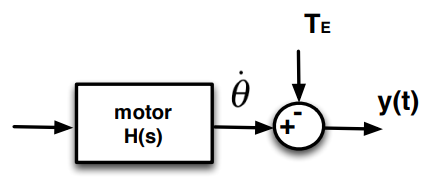
It can now be helpful to draw a full diagram of the system:
  
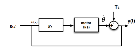
***
Find an expression for $Y(s)$ by converting $y(t)$ and the speed reduction caused by the torque, $\dot{\theta}$, to the Laplace domain:
  
$Y(s) = E(s)K_\mathrm{P}H(s)-\Theta(s)$
  
where $E(s) = R(s)-Y(s)$.
***
Hence:
  
$Y(s) = R(s)K_\mathrm{P}H(s)-Y(s)K_\mathrm{P}H(s)-\Theta(s)$
***
The total steady-state error is caused by both the closed-loop steady-state error and the disturbance error. Hence, both the closed-loop transfer function and the disturbance transfer function need to be calculated.
***
Calculate the closed-loop transfer function by setting $\Theta(s)$ to $0$:
  
$G(s) = \frac{Y(s)}{R(s)} = \frac{K_\mathrm{P}H(s)}{1+K_\mathrm{P}H(s)}$
***
Substituting in $H(s)$:
  
$G(s) = \dfrac{\frac{\frac{20\pi K_\mathrm{P}}{3}}{1+0.01s}}{1+\frac{\frac{20\pi K_\mathrm{P}}{3}}{1+0.01s}}$
***
Tidying up:
  
$G(s) = \frac{20\pi K_\mathrm{P}}{3+0.03s+20\pi K_\mathrm{P}}$
***
Find the closed-loop steady state value:
  
$y_\mathrm{ss} = \lim\limits_{s\rightarrow 0}sG(s)R(s)$
  
$y_\mathrm{ss} = \lim\limits_{s\rightarrow 0} s\cdot \frac{20\pi K_\mathrm{P}}{3+0.03s+20\pi K_\mathrm{P}}\cdot\frac{100}{s}$
***
Simplifying:
  
$y_\mathrm{ss} = \frac{2000\pi K_\mathrm{P}}{3+20\pi K_\mathrm{P}}$
***
Find the closed-loop steady-state error:
  
$e_\mathrm{ss} = r_\mathrm{ss}-y_\mathrm{ss}$
  
$e_\mathrm{ss} = 100-\frac{2000\pi K_\mathrm{P}}{3+20\pi K_\mathrm{P}}$
***
Simplifying:
  
$e_\mathrm{ss} = \frac{300}{3+20\pi K_\mathrm{P}}$
***
Now find an expression for the disturbance transfer function by setting $R(s)$ to $0$:
  
$S(s) = \frac{Y(s)}{\Theta(s)} = \frac{-1}{1+K_\mathrm{P}H(s)}$
***
Substitute in the expression for $H(s)$:
  
$S(s) = \dfrac{-1}{1+\frac{\frac{20}{3}\pi K_\mathrm{P}}{1+0.01s}}$
***
Simplifying:
  
$S(s) = \frac{-3-0.03s}{3+0.03s +20\pi K_\mathrm{P}}$
***
The disturbance steady-state value can be found as follows:
  
$y_\mathrm{Ds} = \lim\limits_{s\rightarrow 0}sS(s)\Theta(s)$
  
$y_\mathrm{Ds} = \lim\limits_{s\rightarrow 0} s\cdot \frac{-3-0.03s}{3+0.03s +20\pi K_\mathrm{P}}\cdot \frac{50}{s}$
***
Simplifying:
  
$y_\mathrm{Ds} = \frac{-150}{3+20\pi K_\mathrm{P}}$
***
Find the disturbance steady-state error:
  
$e_\mathrm{Ds} = 0-y_\mathrm{Ds}$
  
$e_\mathrm{Ds} = \frac{150}{3+20\pi K_\mathrm{P}}$
***
Find the total steady-state error:
  
$e_\mathrm{ts} = e_\mathrm{ss}+e_\mathrm{Ds}$
  
$e_\mathrm{ts} = \frac{300}{3+20\pi K_\mathrm{P}}+\frac{150}{3+20\pi K_\mathrm{P}}= \frac{450}{3+20\pi K_\mathrm{P}}$
***
The total error must not exceed $1\%$:
  
$1>\frac{450}{3+20\pi K_\mathrm{P}}$
***
Solving for $K_\mathrm{P}$:
  
$K_\mathrm{P} > 7.1$
  
  
| The speed of a D.C. motor is governed by a proportional control system with unity feedback. The shaft of the motor is subject to an external torque causing a maximum speed reduction of $50~\mathrm{rad/s}$. What is the value of $K_\mathrm{P}$ needed to sustain the speed within $1\%$ of the desired value $100~\mathrm{rad/s}$?
  

The parameters of the D.C. motor are:
  
$K_\mathrm{e} = 5~\mathrm{V/krpm}$
$K_\mathrm{t} = 4~\mathrm{Ncm/A}$
$R_\mathrm{a} = 2~\Omega$
$J = 0.1~\mathrm{Ncm/krpm}$
$K_\mathrm{f} = 0$ (No frictional losses)
| 72 | 9 | 45 | 45 | 298 | 0 | 16 | 5 | 1 | What is the value of $K_\mathrm{P}$ needed to sustain the speed within $1\%$ of the desired value $100~\mathrm{rad/s}$? | 1 |
05b6833a-94f9-46a4-8e93-018225fb5cd0 | 0 | 0 | 1 | 9 | 4 | 2 | 5 | 0 | Using complex impedances develop the gain and phase shift relationships between the input and output voltages of the passive high-pass filter below and draw a Bode diagram of the filter.
| 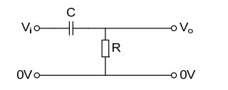
| 1 | 0.666667 | 2 | null | Use the potential divider equation to describe the relationship between input and output voltages:
***
$V_\mathrm{o} = \frac{Z_\mathrm{R}}{Z_\mathrm{R}+Z_\mathrm{C}}V_\mathrm{i}$
  
where $Z_\mathrm{R}$ and $Z_\mathrm{C}$ are the impedances of the resistor and capacitor respectively.
***
From the notes: 
***
$Z_\mathrm{C} = \frac{1}{j\omega C}$
***
$Z_\mathrm{R} = R$ 
***
Substituting the impedances into the potential divider equation:
***
$V_\mathrm{o} = \dfrac{R}{R+\frac{1}{j\omega C}}V_\mathrm{i}$
***
The ratio of the input and output voltages is:
  
$H = \dfrac{V_\mathrm{o}}{V_\mathrm{i}} =\dfrac{R}{R+\frac{1}{j\omega C}}$ 
***
Multiplying by $\frac{j\omega C}{j\omega C}$:
  
$H= \frac{j\omega RC}{j\omega RC + 1}$
***
Taking the magnitude to find the gain:
  
$|H| = \frac{\omega RC}{\sqrt{(\omega RC)^2+1}}$
***
Calculate the phase shift:
  
$\phi = \phi_\mathrm{o}-\phi_\mathrm{i}$
***
$\phi_\mathrm{o} = \tan^{-1}(\frac{\omega RC}{0})= 90^{\circ}$
  
$\phi_\mathrm{i} = \tan^{-1}(\frac{\omega RC}{1}) = \tan^{-1}(\omega RC)$
***
Hence:
  
$\phi = 90^{\circ} - \tan^{-1}(\omega RC)$
***
Bode diagram:
  
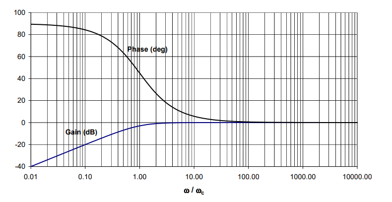  
| Using complex impedances develop the gain and phase shift relationships between the input and output voltages of the passive high-pass filter below and draw a Bode diagram of the filter.

| 31 | 0 | 14 | 14 | 101 | 0 | 1 | 0 | 1 | Using complex impedances develop the gain and phase shift relationships between the input and output voltages of the passive high-pass filter below and draw a Bode diagram of the filter. | 1 |
05dac5a1-05ac-4a85-a191-0221ff134294 | 2 | 0 | 0 | 11 | 4 | 2 | 3 | 5 | A room contains air at $20^{\circ}\mathrm{C}$ and $0.98$ bar with a relative humidity of $85\%$. Determine:
| The partial pressure of the dry-air component.
\nThe specific humidity of the air.
| 2 | 0.333333 | 1 | \n | From the definition of relative humidity:
  
$\phi = \frac{P_\mathrm{v}}{P_\mathrm{sat}(T)}$
***
The saturation pressure, $P_\mathrm{sat}$, at $20^{\circ}\mathrm{C}$, can be found from Data and Formula book (Table E19):
  
$P_\mathrm{sat}(20^{\circ}) = 0.02339$ bar
***
Substituting this value back into the equation for relative humidity:
  
$P_\mathrm{v} = 0.85\times 0.2339 = 0.01988$ bar
***
The total pressure is the sum of the partial pressures of air and vapour. Therefore:
  
$P_\mathrm{a} = P_\mathrm{tot} - P_\mathrm{v}$
***
Substituting in numbers:
  
$P_\mathrm{a} = 0.98-0.01988 = 0.9601$ bar $ = 96.01~\mathrm{kPa} $
\nUsing the equation for specific humidity:
  
$\omega = 0.622\frac{P_\mathrm{v}}{P_\mathrm{a}}$
***
Since both of the partial pressures have been calculated in part (a), they can be substituted in to the above equation:
  
$\omega = 0.622\times\frac{0.01988}{0.9601} = 0.0129$
| A room contains air at $20^{\circ}\mathrm{C}$ and $0.98$ bar with a relative humidity of $85\%$. Determine:
The partial pressure of the dry-air component.
\nThe specific humidity of the air.
| 30 | 3 | 10 | 10 | 102 | 0 | 13 | 0 | 0 | Determine: The partial pressure of the dry-air component. | 1 |
061a2ba6-c482-4891-be40-1a18f21b89bf | 6 | 0 | 0 | 15 | 5 | 0 | 1 | 0 | The Michaelis-Menten equation describes enzyme kinetics.
$$
v=\frac{v_{max}[S]}{K_{M}+[S]}
$$
* $v$ Velocity of enzyme-catalysed reaction ($\mathrm{mmol \cdot s^{-1}}$)
* $v_{max}$ Maximum rate of the reaction ($\mathrm{mmol \cdot s^{-1}}$)
* $K_{M}$ Michaelis constant ($\mathrm{mM}$)
* $[S]$ Concentration of substrate ($\mathrm{mM}$)
| Sketch the graph of this equation: $v$ is the $y$-variable, $[S]$ is the $x$-variable. What is the horizontal limit in terms of its variables?
\nNext, we will prove an important property of the Michalis-Menten equation. Find the value of $v$ when $[S]$=$K_{M}$.
\nThis graph is not very user-friendly as far as extracting $v_{max}$ and $K_{M}$ from a graph is concerned. The Lineweaver-Burk equation is the reciprocal transformation of the Michaelis-Menten equation, which allows us to linearise this equation and easily estimate values for $v_{max}$ and $K_{M}$.
Convert the Michaelis-Menten equation into the Lineweaver-Burk equation by taking reciprocal of both sides, so that the $X$-variable becomes $\frac{1}{[S]}$ and the $Y$-variable becomes $\frac{1}{v}$. What is the $Y$-intercept of this transform?
\nWhat is the gradient of this transform?
\nFinally when plotting this equation we need to consider the units for each axis.
What are the units for the X-axis? (To write a power, use '\*\*', *i.e. *write $x^{-1}$ as 'x\*\*-1')
\nFinally when plotting this equation we need to consider the units for each axis.
What are the units for the Y-axis? (Treat the unit symbols as algebra: use a '\*' to represent a multiplication, *i.e.* write $\mathrm{kg\,m\,s^{-2}}$ as 'kg\*m\*s\*\*-2' or 'kg\*m/s\*\*2'.)
| 6 | 1 | 2 | \n\n\n\n\n | As $[S] \to \infty$ adding the finite value $K_M$ to $[S]$ becomes less and less significant compared to the size of $[S]$ alone. Therefore, $v =\frac{v_{max} [S]}{K_M + [S]} \to \frac{v_{max} [S]}{[S]}=v_{max}$. The horizontal asymptote is therefore at $v=v_{max}$.
  
\nWhen $[S] = K_M$ , then $v =\frac{v_{max} [S]}{[S] + [S]}= \frac{v_{max} [S]}{2[S]}=\frac{v_{max}}{2}$
\n$$
v =\frac{v_{max} [S]}{K_M + [S]}
$$
Take reciprocals:
$$
\frac{1}{v} = \frac{1}{\frac{v_{max} [S]}{K_M + [S]}} = \frac{K_M + [S]}{v_{max} [S]}
$$
Separate sum in numerator:
$$
\frac{1}{v} = \frac{K_M}{v_{max} [S]} + \frac{[S]}{v_{max} [S]}
$$
Cancel terms in $[S]$:
$$
\frac{1}{v} = \frac{K_M \times 1}{v_{max} [S]} + \frac{1}{v_{max}}
$$
Force into $Y=mX+c$ form:
$$
\frac{1}{v} = \frac{K_M}{v_{max}} \times \frac{1}{[S]} + \frac{1}{v_{max}}
$$
The $Y$-intercept is $\frac{1}{v_{max}}$
\nSee previous section for worked solution.
The gradient is $\frac{K_M}{v_{max}}$
\nThe units of the transformed $x$-axis are those of $1/[S]$ , *i.e.* $\mathrm{mM}^{−1}$ (or $\mathrm{L \cdot mmol^{−1}}$),
\nThe units of the transformed $Y$-axis are those of $1/v$*, i.e.* $\mathrm{s \cdot mmol^{−1}}$.
| The Michaelis-Menten equation describes enzyme kinetics.
$$
v=\frac{v_{max}[S]}{K_{M}+[S]}
$$
* $v$ Velocity of enzyme-catalysed reaction ($\mathrm{mmol \cdot s^{-1}}$)
* $v_{max}$ Maximum rate of the reaction ($\mathrm{mmol \cdot s^{-1}}$)
* $K_{M}$ Michaelis constant ($\mathrm{mM}$)
* $[S]$ Concentration of substrate ($\mathrm{mM}$)
Sketch the graph of this equation: $v$ is the $y$-variable, $[S]$ is the $x$-variable. What is the horizontal limit in terms of its variables?
\nNext, we will prove an important property of the Michalis-Menten equation. Find the value of $v$ when $[S]$=$K_{M}$.
\nThis graph is not very user-friendly as far as extracting $v_{max}$ and $K_{M}$ from a graph is concerned. The Lineweaver-Burk equation is the reciprocal transformation of the Michaelis-Menten equation, which allows us to linearise this equation and easily estimate values for $v_{max}$ and $K_{M}$.
Convert the Michaelis-Menten equation into the Lineweaver-Burk equation by taking reciprocal of both sides, so that the $X$-variable becomes $\frac{1}{[S]}$ and the $Y$-variable becomes $\frac{1}{v}$. What is the $Y$-intercept of this transform?
\nWhat is the gradient of this transform?
\nFinally when plotting this equation we need to consider the units for each axis.
What are the units for the X-axis? (To write a power, use '\*\*', *i.e. *write $x^{-1}$ as 'x\*\*-1')
\nFinally when plotting this equation we need to consider the units for each axis.
What are the units for the Y-axis? (Treat the unit symbols as algebra: use a '\*' to represent a multiplication, *i.e.* write $\mathrm{kg\,m\,s^{-2}}$ as 'kg\*m\*s\*\*-2' or 'kg\*m/s\*\*2'.)
| 253 | 27 | 0 | 0 | 158 | 0 | 209 | 18 | 0 | The Michaelis-Menten equation describes enzyme kinetics. What is the horizontal limit in terms of its variables? Find the value of $v$ when $[S]$=$K_{M}$. Convert the Michaelis-Menten equation into the Lineweaver-Burk equation by taking reciprocal of both sides, so that the $\mathrm{mmol \cdot s^{-1}}$0-variable becomes $\mathrm{mmol \cdot s^{-1}}$1 and the $\mathrm{mmol \cdot s^{-1}}$2-variable becomes $\mathrm{mmol \cdot s^{-1}}$3. What is the $\mathrm{mmol \cdot s^{-1}}$2-intercept of this transform? What is the gradient of this transform? Finally when plotting this equation we need to consider the units for each axis. What are the units for the X-axis? To write a power, use '', i.e. write $\mathrm{mmol \cdot s^{-1}}$5 as 'x-1' Finally when plotting this equation we need to consider the units for each axis. What are the units for the Y-axis? Treat the unit symbols as algebra: use a '' to represent a multiplication, i.e. write $\mathrm{mmol \cdot s^{-1}}$6 as 'kgms-2' or 'kgm/s2'. | 13 |
06696572-f255-45b9-bafa-cabbe184e559 | 2 | 1 | 0 | 4 | 3 | 3 | 5 | 0 | A wide freshwater stream has a smooth granular bed with a bed slope of $S = 0.002$, a uniform flow depth of $h =2.0\ \mathrm{m}$ and a median grain size of $d_{50} =2\ \mathrm{mm}$.
You may wish to use [the Shields diagram](https://bb.imperial.ac.uk/webapps/blackboard/execute/content/file?cmd=view\&content_id=_2543151_1\&course_id=_30255_1).
| Compute the bed shear stress, $\tau_0$ $\mathrm{[N/m^2]}$.
\nWhat is the critical bed shear stress, $\tau_{cr}\ \mathrm{[N/m^2]}$, for this channel?
\nIs the channel bed stable in terms of initiation of motion for this flow?
| 3 | 0.333333 | 1 | \n\n | The bed sear stress is computed as: $\tau_0 = \rho g h S = 39.240\ \mathrm{N/m^2}$.
\nThe shear velocity $u_*$ is obtained from
$$
u_* = \sqrt{\dfrac{\tau_0}{\rho}} = \sqrt{\dfrac{39.2}{1000}} = 0.198\ \mathrm{m/s}.
$$
The shear Reynolds number is
$$
\mathrm{Re}_* = \dfrac{u_* d_{50}}{\nu} = \dfrac{0.198\cdot 2 \times 10^{-3}}{10^{-6}} = 396.18.
$$
Using the Shields diagram we can obtain a value for $\theta_{cr}$ for $\mathrm{Re}_* = 396.18$. It is important to remember that the diagram is in semilogarithmic axes. The critical Shields parameter in this case is: $\theta_{cr} \approx 0.058$.
Therefore the critical bed shear stress is
$$
\tau_{cr} = \theta_{cr}\cdot \rho \cdot g (s-1) \cdot d_{50} = 1.88\ \mathrm{N/m^2},
$$
where $s=\rho_s/\rho_w = 2.65$ is the relative sediment density.
\nTo determine whether there will be initiation of motion, the bed shear stress is compared to the critical bed shear stress. Since $\tau_0>\tau_{cr}$, the channel bed is not stable.
| A wide freshwater stream has a smooth granular bed with a bed slope of $S = 0.002$, a uniform flow depth of $h =2.0\ \mathrm{m}$ and a median grain size of $d_{50} =2\ \mathrm{mm}$.
You may wish to use [the Shields diagram](https://bb.imperial.ac.uk/webapps/blackboard/execute/content/file?cmd=view\&content_id=_2543151_1\&course_id=_30255_1).
Compute the bed shear stress, $\tau_0$ $\mathrm{[N/m^2]}$.
\nWhat is the critical bed shear stress, $\tau_{cr}\ \mathrm{[N/m^2]}$, for this channel?
\nIs the channel bed stable in terms of initiation of motion for this flow?
| 70 | 6 | 10 | 10 | 104 | 0 | 34 | 3 | 0 | You may wish to use . Compute the bed shear stress, $\tau_0$ $\mathrm{[N/m^2]}$. What is the critical bed shear stress, $\tau_{cr}\ \mathrm{[N/m^2]}$, for this channel? Is the channel bed stable in terms of initiation of motion for this flow? | 4 |
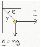
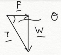
071be152-c0bf-4be1-8a82-3514e08b18ea | 1 | 0 | 0 | 19 | 6 | 1 | 0 | 4 | null | (L2) A weight of mass 10 kg is attached to a wall with a string, and is pulled horizontally with a force $\vec{F}$ so that it is in equilibrium, as in the diagram. Find the magnitude of the force $F$ required for the string to make an angle of $\theta=60^\circ$ to the *normal* to the wall.
| 1 | 0.333333 | 0 | * One approach is to equate vertical and horizontal forces, then solve each equation separately, but actually there is no need to do this; there is a shorter way.
***
* A shorter approach is to draw a triangle, and use trigonometric to solve directly for $F$.
| Redrawing the forces, since the mass is in equilibrium $ \vec{F}+\vec{T}+\vec{W}=0 $.
***
From the triangle, we see that $\tan \theta = \dfrac{W}{F} \quad \rightarrow \quad F = mg / \tan\theta$.
***
For $\theta=60^\circ,$ $F = (10\times9.81)/\tan{60^\circ} = 56.6{N}$.
,
, Horizontal Components:
$$
F=T\cos{\theta}\tag{1}
$$
Vertical Components:
$$
T\sin{\theta}= mg \tag{2}
$$
***
Re-arranging eq. (2) for $T$:
$$
T = mg/\sin{\theta}
$$
***
Inserting this result into eq. (1):
$$
F = \frac{mg}{\sin\theta}\cos\theta = \frac{mg}{\tan\theta} = \frac{10\times9.81}{\tan{60^\circ}}=56.6\text{N}
$$
| null | 1 | 0 | 9 | 9 | 50 | 1 | 56 | 3 | 0 | (L2) A weight of mass 10 kg is attached to a wall with a string, and is pulled horizontally with a force $\vec{F}$ so that it is in equilibrium, as in the diagram. Find the magnitude of the force $F$ required for the string to make an angle of $\theta=60^\circ$ to the *normal* to the wall.

| 0 |
07558792-2199-462d-8f3e-bf701a870259 | 1 | 0 | 0 | 18 | 6 | 1 | 1 | 1 | In Lecture 4 we derived the velocity addition formula for a particle moving with speed $u$ along the $x$ axis, in a frame moving at velocity $v$ in the $x$ direction. If the particle velocity is not just directed along the $x$ axis, then the velocity transformation formula needs to be written as $u_x^\prime = \frac{u_x - v}{1- vu_x/c^2}.$
   
Use the same method as in the lecture to work out the transformation rule for one of the perpendicular velocity components, e.g. $u_y$. | In Lecture 4 we derived the velocity addition formula for a particle moving with speed $u$ along the $x$ axis, in a frame moving at velocity $v$ in the $x$ direction. If the particle velocity is not just directed along the $x$ axis, then the velocity transformation formula needs to be written as $u_x^\prime = \frac{u_x - v}{1- vu_x/c^2}.$
   
Use the same method as in the lecture to work out the transformation rule for one of the perpendicular velocity components, e.g. $u_y$. | 1 | 0.333333 | 2 | How can you write $u'_y$ in terms of $y'$ and $t'$?
***
   
What do you know about the relative direction of $y'$ and $v$? How des this knowledge let us easily relate $y$ and $y'$?
***
   
As $y'$ is perpendicular to $v$, there will be no length contraction in this direction so $y=y'$. Thus, the only coordinate where we need to consider the Lorentz transformation is the time coordinate. The formula for this is given in question 2.1.
***
   
You can use the Lorentz formula to write $t'$ in terms of $x$ and $t$. Remeber that $u'_y = y'/t'$ and $u_x = x/t$.  | We know that $y=u_y t$ and $y^\prime = u_y^\prime t^\prime$. We also know $y^\prime = y$ as the frame only moves in the $x$ direction. 
***
The Lorentz transformation for $t$ only involves the $x$ coordinate for which $x=u_xt$, so this gives
***
   
$$
ct^\prime = \gamma (ct - \beta x) = \gamma \left(ct- \frac{v}{c} u_x t\right)
= \gamma ct \left(1 - \frac{v u_x}{c^2}\right)
$$
***
Hence, the $y$ velocity in the moving frame is
$$
u_y^\prime=\frac{y^\prime}{t^\prime}
=\frac{u_y t}{t^\prime} = \frac{u_y t}{\gamma t(1 - v u_x/c^2)}
=\frac{u_y}{\gamma(1-vu_x/c^2)}
$$
A similar expression holds for $u_z^\prime$. | In Lecture 4 we derived the velocity addition formula for a particle moving with speed $u$ along the $x$ axis, in a frame moving at velocity $v$ in the $x$ direction. If the particle velocity is not just directed along the $x$ axis, then the velocity transformation formula needs to be written as $u_x^\prime = \frac{u_x - v}{1- vu_x/c^2}.$
   
Use the same method as in the lecture to work out the transformation rule for one of the perpendicular velocity components, e.g. $u_y$. | 80 | 7 | 11 | 11 | 60 | 15 | 80 | 7 | 0 | In Lecture 4 we derived the velocity addition formula for a particle moving with speed $u$ along the $x$ axis, in a frame moving at velocity $v$ in the $x$ direction. If the particle velocity is not just directed along the $x$ axis, then the velocity transformation formula needs to be written as $u_x^\prime = \frac{u_x - v}{1- vu_x/c^2}.$ Use the same method as in the lecture to work out the transformation rule for one of the perpendicular velocity components, e.g. | 2 |
09429e36-172e-4f9c-8e4d-206d50606944 | 7 | 0 | 0 | 19 | 6 | 1 | 8 | 1 | **(L14)**: The matrices below represent rotations in $\mathbb{R}^3$ about the $x$-axis ($\text{R}_1$) and about the $y$-axis ($\text{R}_2$), each by 90$^\circ$ in the counter-clockwise direction:
$$
\text{R}_1=
\left(\begin{array}{ccr}
1&\hskip12pt 0&\hskip3pt 0\\
0&\hskip12pt 0&\hskip3pt -1\\
0&\hskip12pt 1&\hskip3pt 0
\end{array}\right)\, ,\qquad
\text{R}_2=
\left(\begin{array}{rcc}
0&\hskip12pt 0&\hskip12pt 1\\
0&\hskip12pt 1&\hskip12pt 0\\
-1&\hskip12pt 0&\hskip12pt 0
\end{array}\right)\, .
$$
| Find the real eigenvalues of $\text{R}_1$ and $\text{R}_2$ (denoted $\lambda_1$, $\lambda_2$ respectively). Determine the normalised eigenvectors corresponding to the eigenvalues.
\nFind the products ${\mathbf{\text{R}}}_1{\mathbf{\text{R}}}_2$ and ${\mathbf{\text{R}}}_2{\mathbf{\text{R}}}_1$ and show they do not commute.
\nDetermine the rotation axes of ${\mathbf{\text{R}}}_1{\mathbf{\text{R}}}_2$ and ${\mathbf{\text{R}}}_2{\mathbf{\text{R}}}_1$ (represent these as normalised eigenvectors $\mathbf{{u}_{12}},\mathbf{{u}_{21}}$), and comment on your results in light of the result in part (b).
| 3 | 0.666667 | 3 | Set up and solve the characteristic equations $p(\lambda)=\det{(\text{R} - \lambda\mathbb{I}_3)}$ for each rotation matrix (see **section 3.19**). 
***
After finding the eigenvalue, in each case solve $(\text{R}- \lambda \mathbb{I}_3)\mathbf{\underline{x}}=0$ for the eigenvector $\mathbf{\underline{x}}=(x,y,z)$...
***
... You may find solutions with no dependency on $x,y$ or $z$. This means that your choice of $x,y$ or $z$ is arbitrary (thus choose $x,y$ or $z$ that give a normalised vector).
\nSee matrix multiplication, **section 3.3**.
\nTake $\text{R}_1\text{R}_2$ and $\text{R}_2\text{R}_1$ from part (b), and calculate their normalised eigenvectors as in part (a). This tells you the rotation axes because rotation axes are invariant under rotations. 
***
Are the eigenvectors you found equivalent? This will verify if $\text{R}_1\text{R}_2$ and $\text{R}_2\text{R}_1$ commute.
| Solving the characteristic equation for $\text{R}_1$ (see section **3.19**). 
***
$$
\det(\text{R}_1-\lambda\mathbb{I}_3)=
\left|\begin{array}{crr}
1-\lambda&0&\hskip3pt 0\\
0&-\lambda&\hskip3pt -1\\
0&1&\hskip3pt -\lambda
\end{array}\right|=\lambda^2(1-\lambda)+(1-\lambda)=(1-\lambda)(\lambda^2+1)=0,
$$
which yields one real eigenvalue $\lambda_1=1$. The corresponding eigenvector $\mathbf{\underline{x}}=(x,y,z)$ is found from solving 
$(\text{R}_1 - \lambda \mathbb{I}_3)\mathbf{\underline{x}}=0$:
***
$$
\begin{aligned}
\left(\begin{array}{crr}
0&\hskip3pt 0&\hskip3pt 0\\
0&\hskip3pt -1&\hskip3pt -1\\
0&\hskip3pt 1&\hskip3pt -1
\end{array}\right)
\left(
\begin{array}{c}
x\\
y\\
z
\end{array}
\right)=
\left(
\begin{array}{r}
0\hskip12pt\\
-y-z\\
y-z
\end{array}
\right)=\left(
\begin{array}{c}
0\\
0\\
0
\end{array}
\right),
\end{aligned}
$$
***
which shows $y=z=0$. However, our choice of $x$ is arbitrary here (it is unaffected by the matrix operation), so we may take as our normalised eigenvector $ \mathbf{\hat{u}}_1=\left(\begin{array}{c}1\\0\\0\end{array}\right) $, which is the $x$-axis (as we expect for a rotation about the $x$-axis).
***
Similarly, for $\text{R}_2$, the eigenvalues are determined from:
***
$$
\det({\mathbf{\text{R}}}_2-\lambda\mathbb{I})=\left|\begin{array}{rcr}-\lambda&\hskip8pt \hskip3pt 0&\hskip3pt 1\\0&\hskip8pt 1-\lambda&\hskip3pt 0\\-1&\hskip8pt 0&\hskip3pt -\lambda\end{array}\right|=\lambda^2(1-\lambda)+(1-\lambda)=(1-\lambda)(\lambda^2+1)=0\,
$$
which yields the real eigenvalue $\lambda_2=1$. The corresponding eigenvector is,
***
$$
\begin{align*}
\left(\begin{array}{crr}
0&\hskip3pt 0&\hskip3pt 0\\
0&\hskip3pt -1&\hskip3pt -1\\
0&\hskip3pt 1&\hskip3pt -1
\end{array}\right)
\left(
\begin{array}{c}
x\\
y\\
z
\end{array}
\right)=
\left(
\begin{array}{r}
0\hskip12pt\\
-y-z\\
y-z
\end{array}
\right)=\left(
\begin{array}{c}
0\\
0\\
0
\end{array}
\right),
\end{align*}
$$
which shows that $x=z=0$, but $y$ is arbitrary, so we may take as our normalised eigenvector $ \mathbf{\hat{u}}_2=\left(\begin{array}{c} 0\\ 1\\ 0\end{array}\right), $ which is the $y$-axis (as we expect for a rotation about the $y$-axis).
\n$$
{\mathbf{\text{R}}}_1{\mathbf{\text{R}}}_2 =\left(\begin{array}{ccr}1&\hskip12pt 0&\hskip3pt 0\\0&\hskip12pt 0&\hskip3pt -1\\0&\hskip12pt 1&\hskip3pt 0\end{array}\right)\left(\begin{array}{rcc}0&\hskip12pt 0&\hskip12pt 1\\0&\hskip12pt 1&\hskip12pt 0\\-1&\hskip12pt 0&\hskip12pt 0\end{array}\right)=\left(\begin{array}{ccc}0&\hskip12pt 0&\hskip12pt 1\\1&\hskip12pt 0&\hskip12pt 0\\0&\hskip12pt 1&\hskip12pt 0\end{array}\right),
$$
***
$$
{\mathbf{\text{R}}}_2{\mathbf{\text{R}}}_1 =\left(\begin{array}{rcc}0&\hskip12pt 0&\hskip12pt 1\\0&\hskip12pt 1&\hskip12pt 0\\-1&\hskip12pt 0&\hskip12pt 0\end{array}\right)\left(\begin{array}{ccr}1&\hskip12pt 0&\hskip3pt 0\\0&\hskip12pt 0&\hskip3pt -1\\0&\hskip12pt 1&\hskip3pt 0\end{array}\right)=\left(\begin{array}{rcr}0&\hskip12pt 1&\hskip3pt 0\\0&\hskip12pt 0&\hskip3pt -1\\-1&\hskip12pt 0&\hskip3pt 0\end{array}\right),
$$
which shows that ${\mathbf{\text{R}}}_1{\mathbf{\text{R}}}_2\ne{\mathbf{\text{R}}}_2{\mathbf{\textsf{R}}}_1$.
\nThe eigenvalues of ${\mathbf{\text{R}}}_1{\mathbf{\text{R}}}_2$ are calculated as:
***
$$
\begin{aligned}
\det({\mathbf{\text{R}}}_1{\mathbf{\text{R}}}_2-\lambda\mathbb{I})=\left|\begin{array}{rrr}
-\lambda&\hskip3pt 0&\hskip3pt 1\\
1&\hskip3pt -\lambda&\hskip3pt 0\\
0&\hskip3pt 1&\hskip3pt -\lambda
\end{array}\right|=-\lambda^3+1=0\, ,
\end{aligned}
$$
so the real eigenvalue is $\lambda=1$, with a corresponding eigenvector,
***
$$
\begin{aligned}
\left(\begin{array}{rrr}
-1&\hskip3pt 0&\hskip3pt 1\\
1&\hskip3pt -1&\hskip3pt 0\\
0&\hskip3pt 1&\hskip3pt -1
\end{array}\right)\left(
\begin{array}{c}
x\\
y\\
z
\end{array}
\right)=
\left(
\begin{array}{r}
-x+z\\
x-y \\
y-z
\end{array}
\right)=\left(
\begin{array}{c}
0\\
0\\
0
\end{array}
\right),
\end{aligned}
$$
***
We have that $x=y=z$. Thus, we may take as our eigenvector $ \mathbf{\hat{u}}_{12}=\dfrac{1}{\sqrt{3}}\left(\begin{array}{c}1\\1\\1\end{array}\right). $
The invariant vector is actually in the $(+x)(+y)(-z)$ quadrant, though it might not look like that in the figure.
Carrying out the same process for $\text{R}_2\text{R}_1$:
***
$$
\det({\mathbf{\text{R}}}_2{\mathbf{\text{R}}}_1-\lambda\mathbb{I})=\left|\begin{array}{rrr}-\lambda&\hskip3pt 1&\hskip3pt 0\\0&\hskip3pt -\lambda&\hskip3pt -1\\-1&\hskip3pt 0&\hskip3pt -\lambda\end{array}\right|=-\lambda^3+1=0.
$$
***
So the real eigenvalue is again: $\lambda=1$. The corresponding eigenvector is given by,
$$
\begin{aligned}
\left(\begin{array}{rrr}
-1&\hskip3pt 1&\hskip3pt 0\\
0&\hskip3pt -1&\hskip3pt -1\\
-1&\hskip3pt 0&\hskip3pt -1
\end{array}\right)\left(
\begin{array}{c}
x\\
y\\
z
\end{array}
\right)=
\left(
\begin{array}{r}
-x+y\\
-y-z\\
-x-z
\end{array}
\right)=\left(
\begin{array}{c}
0\\
0\\
0
\end{array}
\right)\, ,
\end{aligned}
$$
which implies that $x=y=-z$.
Thus, we may take $ \mathbf{\hat{u}}_{21}=\dfrac{1}{\sqrt{3}}\left(\begin{array}{r}1\\1\\-1\end{array}\right) $,
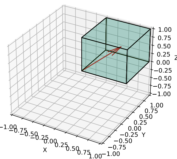
(it might look like it hasn’t moved but the cube has rotated around the eigenvector - hence the slightly different colouring) which again shows the multiplication of ${\mathbf{\text{R}}}_1$ and ${\mathbf{\text{R}}}_2$ does not commute; the different products result in quite different operations.
| **(L14)**: The matrices below represent rotations in $\mathbb{R}^3$ about the $x$-axis ($\text{R}_1$) and about the $y$-axis ($\text{R}_2$), each by 90$^\circ$ in the counter-clockwise direction:
$$
\text{R}_1=
\left(\begin{array}{ccr}
1&\hskip12pt 0&\hskip3pt 0\\
0&\hskip12pt 0&\hskip3pt -1\\
0&\hskip12pt 1&\hskip3pt 0
\end{array}\right)\, ,\qquad
\text{R}_2=
\left(\begin{array}{rcc}
0&\hskip12pt 0&\hskip12pt 1\\
0&\hskip12pt 1&\hskip12pt 0\\
-1&\hskip12pt 0&\hskip12pt 0
\end{array}\right)\, .
$$
Find the real eigenvalues of $\text{R}_1$ and $\text{R}_2$ (denoted $\lambda_1$, $\lambda_2$ respectively). Determine the normalised eigenvectors corresponding to the eigenvalues.
\nFind the products ${\mathbf{\text{R}}}_1{\mathbf{\text{R}}}_2$ and ${\mathbf{\text{R}}}_2{\mathbf{\text{R}}}_1$ and show they do not commute.
\nDetermine the rotation axes of ${\mathbf{\text{R}}}_1{\mathbf{\text{R}}}_2$ and ${\mathbf{\text{R}}}_2{\mathbf{\text{R}}}_1$ (represent these as normalised eigenvectors $\mathbf{{u}_{12}},\mathbf{{u}_{21}}$), and comment on your results in light of the result in part (b).
| 93 | 16 | 38 | 38 | 278 | 13 | 61 | 9 | 0 | $ Find the real eigenvalues of $\text{R}_1$ and $\text{R}_2$ denoted $\lambda_1$, $x$0 respectively. Determine the normalised eigenvectors corresponding to the eigenvalues. Find the products $x$1 and $x$2 and show they do not commute. Determine the rotation axes of $x$1 and $x$2 represent these as normalised eigenvectors $x$5, and comment on your results in light of the result in part b. | 4 |
0b9fe9b9-efd5-40d5-a797-1efe86da2328 | 1 | 0 | 4 | 14 | 4 | 2 | 8 | 1 | Using three-dimensional Cartesian coordinates write all the components of: | $$
\vec{\mathcal{T}}^{\left(\hat{n}\right)}=\underline{\underline{{\sigma}}}^T\hat{n}
$$
\n$$
\vec{\mathcal{T}}^{\left(\hat{\mathrm{e}}_y\right)}=\underline{\underline{\sigma}}^T\hat{\mathrm{e}}_y
$$
\n$$
\mathrm{div}\left(\vec{\mathcal{T}}^{\left(\hat{\mathrm{e}}_y\right)}\right)
$$\n$$
\overrightarrow{\mathrm{div}}\left(\underline{\underline{\sigma}}\right)
$$
\n$$
-\frac{1}{\rho}\overrightarrow{\mathrm{grad}}\left(p\right)+\frac{1}{\rho}\overrightarrow{\mathrm{div}}\left(\underline{\underline{\tau}}\right)
$$
| 5 | 0.5 | 2 | \n\n\n\n | \n\n\n\n | Using three-dimensional Cartesian coordinates write all the components of:$$
\vec{\mathcal{T}}^{\left(\hat{n}\right)}=\underline{\underline{{\sigma}}}^T\hat{n}
$$
\n$$
\vec{\mathcal{T}}^{\left(\hat{\mathrm{e}}_y\right)}=\underline{\underline{\sigma}}^T\hat{\mathrm{e}}_y
$$
\n$$
\mathrm{div}\left(\vec{\mathcal{T}}^{\left(\hat{\mathrm{e}}_y\right)}\right)
$$\n$$
\overrightarrow{\mathrm{div}}\left(\underline{\underline{\sigma}}\right)
$$
\n$$
-\frac{1}{\rho}\overrightarrow{\mathrm{grad}}\left(p\right)+\frac{1}{\rho}\overrightarrow{\mathrm{div}}\left(\underline{\underline{\tau}}\right)
$$
| 18 | 5 | 0 | 0 | 1 | 0 | 9 | 5 | 0 | Using three-dimensional Cartesian coordinates write all the components of:$ \vec{\mathcal{T}}^{\left(\hat{n}\right)}=\underline{\underline{{\sigma}}}^T\hat{n} $ $ \vec{\mathcal{T}}^{\left(\hat{\mathrm{e}}_y\right)}=\underline{\underline{\sigma}}^T\hat{\mathrm{e}}_y $ $ \mathrm{div}\left(\vec{\mathcal{T}}^{\left(\hat{\mathrm{e}}_y\right)}\right) $ $ \overrightarrow{\mathrm{div}}\left(\underline{\underline{\sigma}}\right) $ $ -\frac{1}{\rho}\overrightarrow{\mathrm{grad}}\left(p\right)+\frac{1}{\rho}\overrightarrow{\mathrm{div}}\left(\underline{\underline{\tau}}\right) $ | 1 |
0ba3880d-0abb-480d-a028-280c196df8ca | 1 | 0 | 0 | 17 | 6 | 1 | 2 | 2 | A woman of mass 60 kg stands at one end of a 10 m plank of mass 20 kg, which itself lies on a (frictionless) frozen lake. She walks to the other end of the plank. By using the principle of conservation of momentum, work out how far she has travelled relative to the lake.
\[Those of you who already know about the centre of mass may see an easier way to do this problem, but it is good practice to try it using conservation of momentum only. See *Problem Sheet 4, Question 3* for the centre of mass approach.]
| Distance $x_\text{w}$ travelled by woman relative to lake:
| 1 | 0.666667 | 1 | Call the mass of the woman $m_{\text{w}}$ and her velocity $v_{\text{w}}$. The mass and velocity of the plank are $m_{\text{p}}$ and $v_{\text{p}}$.
***
What is the initial momentum of the system? 
***
Use conservation of momentum to express this in terms of $m_{\text{w}}$, $v_{\text{w}}$, $m_{\text{p}}$, and $v_{\text{p}}$. This should give you an equation for $v_\text{w}$ as a function of the other variables...
***
... Can you express this equation in terms of displacements, $x_\text{w}$ and $x_{\text{p}}$, rather than velocities? ...
***
... You can do this by integration or state the relationship logically.
***
You now know how far the plank moves in one direction if the woman moves in the other direction. Use this to find the distance the woman travels relative to the lake if she walks the entire $10\text{m}$ length of the plank.
| Call the mass of the woman $m_{\text{w}}$ and her velocity $v_{\text{w}}$. The mass and velocity of the plank are $m_{\text{p}}$ and $v_{\text{p}}$. Since no externally applied horizontal forces are acting on the system consisting of the woman and the plank, its total momentum, which starts off equal to zero, must remain equal to zero:
***
$$
m_{\text{w}} v_{\text{w}} + m_{\text{p}} v_{\text{p}} = 0 \quad
\text{at all times.}
\implies v_{\text{p}} = - \frac{m_{\text{w}}}{m_{\text{p}}} v_{\text{w}} = - 3
v_{\text{w}},
$$
where $m_{\text{w}}/m_{\text{p}} = 60$kg$/20$kg $= 3$. 
***
Since the velocities of the woman and plank are always proportional, so are their displacements:
$$
x_{\text{p}} = - 3 x_{\text{w}} .
$$
If you want a more mathematical derivation of the step from $v_{\text{p}} = - 3 v_{\text{w}}$ to $x_{\text{p}} = - 3 x_{\text{w}}$, you can do it using integration:
$$
\begin{aligned}
&v_{\text{p}}(t) = - 3 v_{\text{w}}(t) \\
\Rightarrow \qquad
&\frac{dx_{\text{p}}(t)}{dt} = - 3 \frac{dx_{\text{w}}(t)}{dt} \\
\end{aligned}
$$
$\ldots$
***
$$
\begin{aligned}
\Rightarrow \qquad
&\int_{t'=0}^{t} \frac{dx_{\text{p}}(t')}{dt'} dt' =
- 3 \int_{t'=0}^{t} \frac{dx_{\text{w}}(t')}{dt'} dt' \\
\Rightarrow \qquad
&\left [ x_{\text{p}}(t') \right ]_{0}^{t} = - 3 \left [
x_{\text{w}}(t') \right ]_{0}^{t} \\
\Rightarrow \qquad
& x_{\text{p}}(t) = - 3 x_{\text{w}}(t).
\end{aligned}
$$
It is not necessary to assume that the woman walks at a constant speed.
***
These displacements are measured relative to the frozen lake. For every 1 m the woman moves to the right, the plank moves 3 m to the left, and the woman progresses 4 m along the plank. 
***
By the time she reaches the far end of the 10 m long plank, she has moved 2.5 m to the right and the plank has moved 7.5 m to the left. The woman has travelled 2.5 m relative to the lake.
| A woman of mass 60 kg stands at one end of a 10 m plank of mass 20 kg, which itself lies on a (frictionless) frozen lake. She walks to the other end of the plank. By using the principle of conservation of momentum, work out how far she has travelled relative to the lake.
\[Those of you who already know about the centre of mass may see an easier way to do this problem, but it is good practice to try it using conservation of momentum only. See *Problem Sheet 4, Question 3* for the centre of mass approach.]
Distance $x_\text{w}$ travelled by woman relative to lake:
| 105 | 1 | 14 | 14 | 194 | 12 | 8 | 1 | 0 | By using the principle of conservation of momentum, work out how far she has travelled relative to the lake. Those of you who already know about the centre of mass may see an easier way to do this problem, but it is good practice to try it using conservation of momentum only. See Problem Sheet 4, Question 3 for the centre of mass approach. | 3 |
0ba7ab1f-f9af-439a-b379-e4b2a1fb959f | 1 | 0 | 0 | 9 | 4 | 2 | 6 | 11 | Find the value of the capacitor $C$ needed in the circuit below to ensure a step response faster than $2~\mathrm{ms}$. The resistor values are $R_1 = 1~\mathrm{k\Omega}$ and $R_2 = 4~\mathrm{k\Omega}$.
| 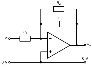
| 1 | 0.666667 | 1 | null | The circuit shown is an active low-pass filter, for which the transfer function can be written as follows:
  
$|H| = \frac{R_2}{R_1}\frac{1}{\sqrt{1+(\omega R_2C)^2}}$
***
This can be re-written in complex form:
  
$|H| = \frac{R_2}{R_1}\frac{1}{1+j\omega R_2C}$
***
Setting $s = j\omega$:
  
$|H| = \frac{R_2}{R_1}\frac{1}{1+R_2Cs}$
***
Hence:
  
$K = \frac{R_2}{R_1}$
  
$\tau = R_2C$
***
To ensure a step response faster than $2~\mathrm{ms}$:
  
$0.002> R_2C$
***
Substituting in the value of $R_2$ and rearranging to find $C$:
  
$C < 0.5~\mu\mathrm{F}$
  
| Find the value of the capacitor $C$ needed in the circuit below to ensure a step response faster than $2~\mathrm{ms}$. The resistor values are $R_1 = 1~\mathrm{k\Omega}$ and $R_2 = 4~\mathrm{k\Omega}$.

| 30 | 4 | 11 | 11 | 70 | 0 | 1 | 0 | 1 | Find the value of the capacitor $C$ needed in the circuit below to ensure a step response faster than $2~\mathrm{ms}$. | 1 |
0bed6097-529a-4f4e-8d35-2734a1d1c0c4 | 1 | 2 | 0 | 17 | 6 | 1 | 0 | 6 | Using a torsion balance, Roll, Krotkov and Dicke [Ann. Phys. **26**(3), 442 (1963)] established the equality of gravitational and inertial mass, $m_G$ and $m_I$, to an accuracy of 3 parts in $10^{11}$.
| Suppose that $m^{\text{Cu}}_{G}/m^{\text{Cu}}_{I} = 1$ but $m^{\text{Pb}}_{G}/m^{\text{Pb}}_{I} = 1 + 3 \times 10^{-11}$. If copper and lead balls were dropped together from the top of the Tower of Pisa, which would hit the ground first?
\nGiven that the tower is 60 m high, what is the separation of the two balls when the first hits the ground? Ignore all forces other than gravity.
\nWould the separation change if you moved the Tower of Pisa to the Moon, where $g$ is approximately six times smaller than on Earth? If so, by what factor would it change?
| 3 | 0.666667 | 3 | The gravitational force uses the gravitational mass $m_G$, whereas N2 uses inertial mass $m_I$. 
***
The gravitational force is equal to the N2 force. Hence solve for the 'inertial' acceleration $a$ of N2.
***
This should tell you which ball accelerates faster, and therefore which ball hits the ground first. 
\nUsing SUVAT equations entirely algebraically at first...
***
... What is the time taken for the lead ball to hit the ground? ...
***
... What distance does the copper ball travel in this time? 
***
... Hence, what is the height $\Delta s$ of the copper ball above the ground?
***
Your expression should contain the relative acceleration of the two particles $a_{\text{Cu}}/{a_{\text{Pb}}}= [1 + (3 \times 10^{-11})]^{-1}$...
***
Since $3\times 10^{-11}$ is exceedingly small, your calculator will not process it when added with $1$. Therefore, perform a binomial expansion to find $a_{\text{Cu}}/{a_{\text{Pb}}}$ analytically.
***
Hence find $\Delta s$.
\nIn your analysis from part (b), did $g$ affect the final answer?
| The acceleration $a$ of a falling object with inertial mass $m_I$ and gravitational mass $m_G$ is given by
***
$$
F = m_G g = m_I a \qquad \Rightarrow \qquad
a = \frac{m_G g}{m_I}.
$$
***
The value of $m_G/m_I$ is larger for lead, so $a_{\text{Pb}} > a_{\text{Cu}}$ and the lead ball hits the ground first.
\nThe lead ball is dropped from the top of the tower of height $h = 60,$m at time $t=0,$s and falls with constant acceleration $a_{\text{Pb}}$ until it hits the ground at time:
***
$$
t_{\text{Pb}} = \sqrt{\frac{2h}{a_{\text{Pb}}}} .
$$
At this exact time, the Cu ball has dropped a distance:
***
$$
s_{\text{Cu}} = \frac{1}{2} a_{\text{Cu}} t_{\text{Pb}}^2 =
\frac{a_{\text{Cu}} h}{a_{\text{Pb}}}.
$$
***
The distance it still has to go (which is the separation of the two balls when the first hits the ground) is:
***
$$
\Delta s = h - s_{\text{Cu}} = \left ( 1 -
\frac{a_{\text{Cu}}}{a_{\text{Pb}}} \right ) h.
$$
***
We are told that $m_G / m_I = 1$ for Cu and $1 + 3 \times 10^{-11}$ for Pb, so
$$
\frac{a_{\text{Cu}}}{a_{\text{Pb}}} = \frac{1}{1 + (3 \times
10^{-11})} = [1 + (3 \times 10^{-11})]^{-1} .
$$
***
Using the binomial (or Taylor) expansion to express this number (the reason why you shouldn't just use a calculator/Python is explained at the end): 
***
$$
\begin{aligned}
(1 + x)^{-1}
&= 1 + (-1)x + \frac{(-1)(-2)}{2!}x^2 + \frac{(-1)(-2)(-3)}{3!} x^3
+ \ldots \\
&= 1 - x + x^2 - x^3 + \ldots ,
\end{aligned}
$$
***
with $x = 3 \times 10^{-11}$ gives
$$
\begin{aligned}
\frac{a_{\text{Cu}}}{a_{\text{Pb}}}
&= 1 - (3\times 10^{-11}) + (3 \times
10^{-11})^2 - (3 \times 10^{-11})^3 + \ldots \\
&\approx 1 - (3 \times 10^{-11}).
\end{aligned}
$$
The approximation in the last line is *very* good because $3
\times 10^{-11}$ is such a small number. Hence:
***
$$
\Delta s \approx 3 \times 10^{-11} h = 1.8 \times 10^{-9}\, \text{m}
= 1.8\,\text{nm}.
$$
***
You might wonder why we used a power expansion? Why not just work out the value of $60 \left ( 1 - \frac{1}{1 + 3 \times 10^{-11}} \right )$ using a calculator or the Python interpreter? That method works fine in this example, but if the $3 \times 10^{-11}$ is replaced by $3 \times 10^{-20}$, Python says the result is exactly zero (try it and see). The problem is that $1/(1 + 3\times 10^{-20}) = 1 - 3\times 10^{-20} + \ldots$ is so close to 1 that computers and calculators, which only keep a finite number of significant figures (around 14 in the case of Python), cannot tell the difference. When working with numbers of very different magnitudes, it is safer to expand in powers of the small number *before* using a computer or calculator.
\n The value of $g$ cancels out of the analysis above so the separation on the Moon would be the same as on Earth.
| Using a torsion balance, Roll, Krotkov and Dicke [Ann. Phys. **26**(3), 442 (1963)] established the equality of gravitational and inertial mass, $m_G$ and $m_I$, to an accuracy of 3 parts in $10^{11}$.
Suppose that $m^{\text{Cu}}_{G}/m^{\text{Cu}}_{I} = 1$ but $m^{\text{Pb}}_{G}/m^{\text{Pb}}_{I} = 1 + 3 \times 10^{-11}$. If copper and lead balls were dropped together from the top of the Tower of Pisa, which would hit the ground first?
\nGiven that the tower is 60 m high, what is the separation of the two balls when the first hits the ground? Ignore all forces other than gravity.
\nWould the separation change if you moved the Tower of Pisa to the Moon, where $g$ is approximately six times smaller than on Earth? If so, by what factor would it change?
| 119 | 6 | 25 | 25 | 312 | 10 | 87 | 3 | 0 | Using a torsion balance, Roll, Krotkov and Dicke Ann. Suppose that $m^{\text{Cu}}_{G}/m^{\text{Cu}}_{I} = 1$ but $m^{\text{Pb}}_{G}/m^{\text{Pb}}_{I} = 1 + 3 \times 10^{-11}$. If copper and lead balls were dropped together from the top of the Tower of Pisa, which would hit the ground first? Given that the tower is 60 m high, what is the separation of the two balls when the first hits the ground? Ignore all forces other than gravity. Would the separation change if you moved the Tower of Pisa to the Moon, where $g$ is approximately six times smaller than on Earth? If so, by what factor would it change? | 7 |
0bf0e821-13b2-4de7-9c7c-2c2cf4b5c13b | 6 | 0 | 0 | 8 | 4 | 2 | 5 | 0 | A steel pipe with $0.125 \text{ m}$ internal diameter, wall thickness $10 \text{ mm}$, is subjected to an internal pressure of $11.0\text{ MPa}$. Use the notation: $K=\frac{r_\text{o}}{r_\text{i}}$ ratio of outer radius to inner radius, $P=$ internal pressure, and external pressure $=0$.
| What are the maximum hoop, radial and shear stresses, if the axial stress is zero **when treated as a thin cylinder**.
\nWhat are the maximum hoop, radial and shear stresses, if the axial stress is zero **when treated as a thick cylinder**. 
   
Show that the maximum hoop stress is given by: $\sigma_\theta=P\frac{K^2+1}{K^2-1}$.
| 2 | 0.333333 | 3 | \n | When using the thin-walled assumption and equations from ME1-SAN:
   
$$
\sigma_\theta=\frac{Pr}{t}=\frac{11\times0.0625}{0.01}=\boxed{68.75\text{ MPa}}
$$
   
***
For thin-walled assumption, because $r>>t$, the radial stress is negligible:
   
$$
\sigma_r=\boxed{0 \text{ MPa}}
$$
   
***
And the maximum shear stress (using the Tresca failure criterion):
   
$$
\hat{\tau}=\frac{\sigma_\theta-\sigma_r}{2}=\boxed{34.38\text{ MPa}}
$$
\nUsing the following equations from the Data & Formulae Booklet for thick-walled analysis:
   
$$
\begin{align}
\sigma_r=A-\frac{B}{r^2}~~~~~~~~~~~~~~~~\sigma_\theta=A+\frac{B}{r^2}
\end{align}
$$
   
***
For an internally pressurised cylinder, the following boundary conditions are applied:
   
$$
\begin{align}
\sigma_r=-&P \text{ at }r=r_i \\
\sigma_r=0&\text{ at }r=r_o
\end {align}
$$
   
***
So:
   
$$
\begin{align}
A-\frac{B}{r_\text{i}^2}=P~~~~~~~~~~~~A-\frac{B}{r_\text{o}^2}=0
\end{align}
$$
   
***
Solving the equations simultaneously for $A$ and $B$:
   
$$
\begin{align}
A=\frac{P}{\frac{r_\text{o}^2}{r_\text{i}^2}-1}~~~~~~~~~~~~~~B=\frac{Pr_\text{o}^2}{\frac{r_\text{o}^2}{r_\text{i}^2}-1}
\end{align}
$$
   
***
Then substituting $K=\frac{r_\text{o}^2}{r_\text{i}^2}$:
   
$$
\begin{align}
A=\frac{P}{K^2-1}~~~~~~~~~~~~~~B=\frac{Pr_\text{o}^2}{K^2-1}
\end{align}
$$
   
***
Substituting $A$ and $B$ back into $(1)$:
   
$$
\begin{align}
\sigma_r=\frac{P}{K^2-1}(1-\frac{r_\text{o}^2}{r^2})\\
~~~~~~~~~~~~~~~~\nonumber\\
\sigma_\theta=\frac{P}{K^2-1}(1+\frac{r_\text{o}^2}{r^2})\\
\end{align}
$$
   
***
As such, $\sigma_\theta$ can be expressed as equation $(9)$ when $r=r_\text{i}$ and substituting $K$.
   
$$
\begin{align}
\sigma_\theta=P\frac{K^2+1}{K^2-1}
\end{align}
$$
   
***
For an internally pressurised cylinder, the max hoop, radial, and hence shear stresses are at the bore $(r=r_\text{i})$.
   
***
Using equation $(8)$ to find hoop stress:
   
$$
\begin{align}
\sigma_\theta&=\frac{P}{K^2-1}(1+\frac{r_\text{o}^2}{r_\text{i}^2}) \\
\nonumber &=\frac{11\times10^6}{(\frac{0.0725}{0.0625})^2-1}(1+\frac{0.0725^2}{0.0625^2})\\
\nonumber &=\boxed{74.66\text{ MPa}}
\end{align}
$$
   
***
Simplifying and using equation $(8)$ to find radial stress:
   
$$
\begin{align}
\sigma_r&=-P =\boxed{-11.0 \text{ MPa}}
\end{align}
$$
   
***
Finally, the maximum shear stress using the Tresca failure criteria can be calculated as:
   
$$
\hat{\tau}=\frac{\sigma_\theta-\sigma_r}{2}=\boxed{42.83\text{ MPa}}
$$
| A steel pipe with $0.125 \text{ m}$ internal diameter, wall thickness $10 \text{ mm}$, is subjected to an internal pressure of $11.0\text{ MPa}$. Use the notation: $K=\frac{r_\text{o}}{r_\text{i}}$ ratio of outer radius to inner radius, $P=$ internal pressure, and external pressure $=0$.
What are the maximum hoop, radial and shear stresses, if the axial stress is zero **when treated as a thin cylinder**.
\nWhat are the maximum hoop, radial and shear stresses, if the axial stress is zero **when treated as a thick cylinder**. 
   
Show that the maximum hoop stress is given by: $\sigma_\theta=P\frac{K^2+1}{K^2-1}$.
| 94 | 7 | 27 | 27 | 215 | 0 | 55 | 1 | 0 | Use the notation: $K=\frac{r_\text{o}}{r_\text{i}}$ ratio of outer radius to inner radius, $P=$ internal pressure, and external pressure $=0$. What are the maximum hoop, radial and shear stresses, if the axial stress is zero when treated as a thin cylinder. What are the maximum hoop, radial and shear stresses, if the axial stress is zero when treated as a thick cylinder. Show that the maximum hoop stress is given by: $\sigma_\theta=P\frac{K^2+1}{K^2-1}$. | 4 |
0c44ba33-2e71-4e4f-9ea3-d60b94200685 | 1 | 1 | 0 | 17 | 6 | 1 | 4 | 4 | Any object moving in a circle is continuously being accelerated towards the centre with centripetal acceleration is given by the formula
$$
a_{\text{centripetal}} = -\omega^2 r = -\frac{v_{\phi}^2}{r},
$$
where $\omega = v_{\phi}/r$ is the angular velocity and $v_{\phi}$ is the speed of the mass around the circumference of the circle.
  
The video linked from the image below shows an Imperial College physics student doing a simple experiment with a pendulum.
[https://www.youtube.com/watch?v=19TKQ7\_lAHA](https://www.youtube.com/watch?v=19TKQ7_lAHA "https://www.youtube.com/watch?v=19TKQ7_lAHA")  
Analyse the experiment mathematically, assuming for simplicity that the string has been replaced by a light but stiff rod so that the starting angle can range from $0$ to $\pi$ radians. Using energy conservation and the concept of centripetal acceleration, find a formula for the minimum angle of release required for a smaller mass $m$ to lift a larger mass $M$. What is the smallest mass $m$ capable of lifting $M$? Does the length of the rod matter?
| Any object moving in a circle is continuously being accelerated towards the centre with centripetal acceleration is given by the formula
$$
a_{\text{centripetal}} = -\omega^2 r = -\frac{v_{\phi}^2}{r},
$$
where $\omega = v_{\phi}/r$ is the angular velocity and $v_{\phi}$ is the speed of the mass around the circumference of the circle.
  
The video linked from the image below shows an Imperial College physics student doing a simple experiment with a pendulum.
[https://www.youtube.com/watch?v=19TKQ7\_lAHA](https://www.youtube.com/watch?v=19TKQ7_lAHA "https://www.youtube.com/watch?v=19TKQ7_lAHA")  
Analyse the experiment mathematically, assuming for simplicity that the string has been replaced by a light but stiff rod so that the starting angle can range from $0$ to $\pi$ radians. Using energy conservation and the concept of centripetal acceleration, find a formula for the minimum angle of release required for a smaller mass $m$ to lift a larger mass $M$. What is the smallest mass $m$ capable of lifting $M$? Does the length of the rod matter?
| 1 | 0.666667 | 4 | How can you use Conservation of Energy to get an expression for the velocity of the mass as a function of $\theta$ after it is released from rest at a starting angle of $\theta_0$? At what value of $\theta$ is the speed of the mass greatest?
***
What force is responsible for lifting the larger mass? Can you write an expression for this force in terms of the angle $\theta$? It may help to resolve the forces on the smaller mass along the direction parallel to the stiff rod. 
***
What condition must the tension satisfy in order for the larger mass to be lifted? Can you use this condition to create an inequality involving $\theta$, $m$ and $M$? If we want to find the smallest mass, $m$, capable of lifting $M$, from which angle must we release $m$?
***
Does your inequality involve the length of the rod? Why does it matter that we use a stiff rod, rather than a string?
| As it swings down to the bottom, the mass $m$ loses gravitational potential energy $mgl(1 - \cos\theta)$. By energy conservation, this must be equal to its kinetic energy $K$ at the bottom of the swing:
$$
K = mgl(1 - \cos\theta).
$$
Since $K = \frac{1}{2}mv^2$, the speed $v_{\phi}$ of the mass at the bottom of the swing is
$$
v_{\phi} = \sqrt{\frac{2K}{m}} = \sqrt{2gl(1 - \cos\theta)}.
$$
***
The mass is not accelerating horizontally when it reaches the bottom of the swing (because there are no horizontal forces acting there) but it still has a centripetal acceleration,
$$
a_{\text{centripetal}} = \frac{v_{\phi}^2}{l} = 2g(1 - \cos\theta),
$$
vertically upwards. The forces acting on the mass are the tension $T$ upwards and the force of gravity $mg$ downwards. Applying Newton's Second Law vertically,
$$
m a_{\text{centripetal}} = T - mg ,
$$
tells us the tension
$$
T = mg + m a_{\text{centripetal}} = m(g + 2g(1 - \cos\theta))
= 3mg - 2mg\cos\theta.
$$
If $\theta = 0$ (the pendulum is just hanging there, stationary and vertical), then $\cos\theta = 1$ and the formula for the tension becomes $T = mg$, which seems sensible. As $\theta$ increases from $0$ to $\pi$, $\cos\theta$ decreases and $T$ rises, which also seems right.
***
For the smaller mass to lift the larger mass, $T$ must be greater than $Mg$, so
$$
\begin{aligned}
&& 3mg - 2mg\cos\theta &> Mg &&\\
\Rightarrow && 2mg\cos\theta &< 3mg - Mg &&\\
\Rightarrow && \theta &> \cos^{-1}\left ( \frac{3m - M}{2m} \right
). &&
\end{aligned}
$$
  
The maximum possible value of $T$ occurs when the release angle $\theta
= \pi$, so that $\cos\theta = -1$. This gives
$$
T_{\text{max}} = 5mg.
$$
If allowed to swing the full 180$^\circ$, a pendulum of mass $m$ would just about be able to lift a mass $5m$. Equivalently, a pendulum with a bob of mass $m$ is capable of lifting a larger mass $M$ as long as $m >
M/5$.
***
The length of the rod does not matter. Although doubling the length doubles the KE (and thus the value of $v_{\phi}^2$) at the bottom of the swing, the maximum centripetal acceleration $v_{\phi}^2/l$ is unaffected.
  
\[If the pendulum had a string instead of a stiff light rod, the string would not remain taut if the bob was released at any angle $\theta > \pi/2$, complicating the analysis. If released from angle $\pi/2$, the swinging mass $m$ would just about be able to lift a mass $M = 3m$.]
| Any object moving in a circle is continuously being accelerated towards the centre with centripetal acceleration is given by the formula
$$
a_{\text{centripetal}} = -\omega^2 r = -\frac{v_{\phi}^2}{r},
$$
where $\omega = v_{\phi}/r$ is the angular velocity and $v_{\phi}$ is the speed of the mass around the circumference of the circle.
  
The video linked from the image below shows an Imperial College physics student doing a simple experiment with a pendulum.
[https://www.youtube.com/watch?v=19TKQ7\_lAHA](https://www.youtube.com/watch?v=19TKQ7_lAHA "https://www.youtube.com/watch?v=19TKQ7_lAHA")  
Analyse the experiment mathematically, assuming for simplicity that the string has been replaced by a light but stiff rod so that the starting angle can range from $0$ to $\pi$ radians. Using energy conservation and the concept of centripetal acceleration, find a formula for the minimum angle of release required for a smaller mass $m$ to lift a larger mass $M$. What is the smallest mass $m$ capable of lifting $M$? Does the length of the rod matter?
| 145 | 9 | 38 | 38 | 354 | 10 | 145 | 9 | 1 | Any object moving in a circle is continuously being accelerated towards the centre with centripetal acceleration is given by the formula $ a_{\text{centripetal}} = -\omega^2 r = -\frac{v_{\phi}^2}{r}, $ where $\omega = v_{\phi}/r$ is the angular velocity and $v_{\phi}$ is the speed of the mass around the circumference of the circle. Analyse the experiment mathematically, assuming for simplicity that the string has been replaced by a light but stiff rod so that the starting angle can range from $0$ to $\pi$ radians. Using energy conservation and the concept of centripetal acceleration, find a formula for the minimum angle of release required for a smaller mass $m$ to lift a larger mass $M$. What is the smallest mass $m$ capable of lifting $M$? Does the length of the rod matter? | 5 |
0c714910-48e8-4c59-bed0-de230105e923 | 3 | 0 | 0 | 15 | 5 | 0 | 0 | 1 | The amount of oxygen and blood pumped by the mammalian heart can be modelled by the following:
$$
V_{O_{2}}=Q(C_{a}-C_{v})
$$
$$
Q=f\cdot S
$$
* $V_{O_{2}}$ Volume of oxygen consumed $(\mathrm{ml\cdot min^{-1}})$
* $Q$ Cardiac output ($\mathrm{mL \cdot min^{-1}}$)
* $C_{a}$ Oxygen content in arterial blood ($\mathrm{mL \, O_{2} \cdot mL \, blood^{-1}}$)
* $C_{v}$ Oxygen content in venous blood ($\mathrm{mL \, O_{2} \cdot mL \, blood^{-1}}$)
* $f$ Heartbeat frequency ($\mathrm{min^{-1}}$)
* $S$ Stroke volume ($\mathrm{mL}$)
By rearranging these equations, we can work out a value for the stroke volume, $S$, of the heart, which is more difficult to measure directly than the other variables.
| Rearrange the second equation, $Q = f S$ so that we could work out stroke volume when cardiac output and heartbeat frequency are known.
\nRearrange the equations so we can calculate stroke volume if we know the difference in oxygen content between arterial and venous blood, as well as the volume of oxygen consumed and the heartbeat frequency? (*i.e.* combine the two equations and solve for $S$).
\nIf the difference in oxygen content between arterial and venous blood is $0.1\,\mathrm{mL \, O_{2} \cdot mL \, blood^{-1}}$, the heartbeat frequency is $1\,\mathrm{s^{-1}}$ and the oxygen consumption rate is $420\,\mathrm{mL\cdot min^{-1}}$, what is the stroke volume of the heart?
| 3 | 1 | 1 | \n\n | $$
Q=S\cdot f
$$
Divide through by $f$
$$
\frac{Q}{f}=\frac{S f}{f}
$$
Cancel $f$ in fraction on RHS:
$$
\frac{Q}{f}=S
$$
Swap LHS and RHS
$$
S=\frac{Q}{f}
$$
\n$$
S=\frac{Q}{f}
$$
And
$$
V_{O_{2}}=Q(C_{a}-C_{v})
$$
Rearrange second for $Q$:
$$
Q=\frac{V_{O_{2}}}{(C_{a}-C_{v})}
$$
Substitute in this value for $Q$ to the first equation:
$$
S=\frac{Q}{f}=\frac{\frac{V_{O_{2}}}{(C_{a}-C_{v})}}{f}
$$
Combine the two denominators:
$$
S=\frac{V_{O_{2}}}{f(C_a-C_v)}
$$
\n$$
S=\frac{420\,\mathrm{mL\,min^{-1}}}{1\,\mathrm{s^{-1}} \times 60\,\mathrm{s\,min^{-1}}\times0.1}=70\,\mathrm{mL}
$$
| The amount of oxygen and blood pumped by the mammalian heart can be modelled by the following:
$$
V_{O_{2}}=Q(C_{a}-C_{v})
$$
$$
Q=f\cdot S
$$
* $V_{O_{2}}$ Volume of oxygen consumed $(\mathrm{ml\cdot min^{-1}})$
* $Q$ Cardiac output ($\mathrm{mL \cdot min^{-1}}$)
* $C_{a}$ Oxygen content in arterial blood ($\mathrm{mL \, O_{2} \cdot mL \, blood^{-1}}$)
* $C_{v}$ Oxygen content in venous blood ($\mathrm{mL \, O_{2} \cdot mL \, blood^{-1}}$)
* $f$ Heartbeat frequency ($\mathrm{min^{-1}}$)
* $S$ Stroke volume ($\mathrm{mL}$)
By rearranging these equations, we can work out a value for the stroke volume, $S$, of the heart, which is more difficult to measure directly than the other variables.
Rearrange the second equation, $Q = f S$ so that we could work out stroke volume when cardiac output and heartbeat frequency are known.
\nRearrange the equations so we can calculate stroke volume if we know the difference in oxygen content between arterial and venous blood, as well as the volume of oxygen consumed and the heartbeat frequency? (*i.e.* combine the two equations and solve for $S$).
\nIf the difference in oxygen content between arterial and venous blood is $0.1\,\mathrm{mL \, O_{2} \cdot mL \, blood^{-1}}$, the heartbeat frequency is $1\,\mathrm{s^{-1}}$ and the oxygen consumption rate is $420\,\mathrm{mL\cdot min^{-1}}$, what is the stroke volume of the heart?
| 197 | 20 | 14 | 14 | 46 | 0 | 100 | 5 | 0 | The amount of oxygen and blood pumped by the mammalian heart can be modelled by the following: $ V_{O_{2}}=Q(C_{a}-C_{v}) $ $ Q=f\cdot S $ $V_{O_{2}}$ Volume of oxygen consumed $(\mathrm{ml\cdot min^{-1}})$ $Q$ Cardiac output $\mathrm{mL \cdot min^{-1}}$ $C_{a}$ Oxygen content in arterial blood $\mathrm{mL \, O_{2} \cdot mL \, blood^{-1}}$ $C_{v}$ Oxygen content in venous blood $\mathrm{mL \, O_{2} \cdot mL \, blood^{-1}}$ $ Q=f\cdot S $0 Heartbeat frequency $ Q=f\cdot S $1 $ Q=f\cdot S $2 Stroke volume $ Q=f\cdot S $3 By rearranging these equations, we can work out a value for the stroke volume, $ Q=f\cdot S $2, of the heart, which is more difficult to measure directly than the other variables. Rearrange the second equation, $ Q=f\cdot S $5 so that we could work out stroke volume when cardiac output and heartbeat frequency are known. Rearrange the equations so we can calculate stroke volume if we know the difference in oxygen content between arterial and venous blood, as well as the volume of oxygen consumed and the heartbeat frequency? combine the two equations and solve for $ Q=f\cdot S $2. If the difference in oxygen content between arterial and venous blood is $ Q=f\cdot S $7, the heartbeat frequency is $ Q=f\cdot S $8 and the oxygen consumption rate is $ Q=f\cdot S $9, what is the stroke volume of the heart? | 5 |
0c82de4f-4a34-49dd-9d48-1605e94b1af5 | 1 | 1 | 0 | 2 | 1 | 2 | 2 | 4 | Manometers are instruments used to measure pressure based on columns of liquid. The figure below shows a u-bend manometer, usually used to measure small pressures.
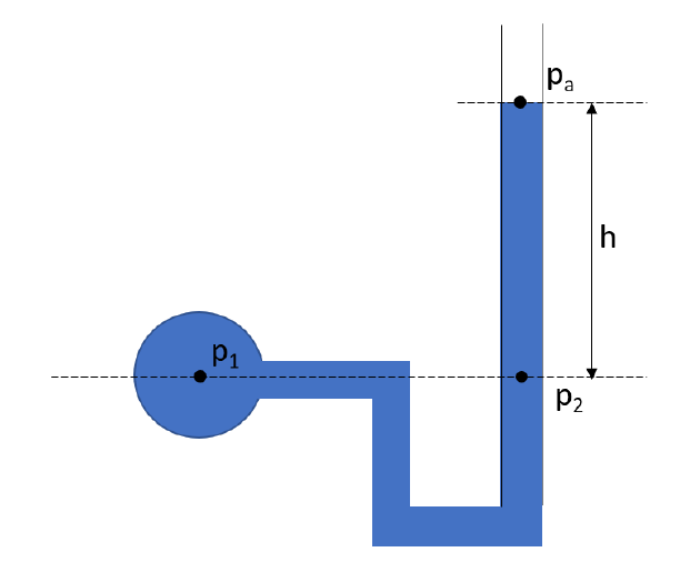
| What is the relationship between the pressures $p_1\,$and $p_2$?
\nWhat is the pressure at $p_2\,$and hence at $p_1$?. You can assume that the fluid in the manometer is water with density $\rho=1000\,$kg/m$^3\,$and $h=10\,$cm.
| 2 | 0.333333 | 1 | \n$\frac{\delta p}{\delta z}=-\rho g$. Solve this to find an expression for $p$.
***
By integration we get $p=-\rho gz +p_0$. To find the value of the constant $p_0$ we can set $z=0$ at the top of the pipe, where the pressure is atmospheric pressure, $p_a$. 
Substitute $p_o$ into the equation for $p$ that you found to get a general equation for pressure.
***
You should find that $p_0=p_a$ and that $P=-\rho gz +p_a$. At point 2 the $z$ co-ordinate is $-h$ (note we are measuring the height h downwards from the top of the pipe so it is in a negative direction),
Using this and the general equation for pressure, find an equation for $p_2$
***
You should find that $p_2=-\rho g(-h) +p_a$. Taking $p_a= 101$ kPa and $g=9.81$ m/s$^2$ find $p_2$.
Use this and the relationship between $p_1$ and $p_2$ from the previous part to find the value for $p_1$.
***
Convert the value of $p_1$ to a gauge pressure.
| \n$\frac{\delta p}{\delta z}=-\rho g$ so integrating we get $P=-\rho gz +P_0$
To find the value of the constant $P_0$ we can set $z=0$ at the top of the pipe, where the pressure is atmospheric pressure, $p_a$. Then we substitute these values for pressure and $z$ into the general equation $P=-\rho gz +P_0=p_a=0+P_0$ and so $P_0$ must equal $p_a$. The general equation for pressure can then be written $P=-\rho gz +p_a$
At point 2 the $z$ co-ordinate is $-h$ (note we are measuring the height h downwards from the top of the pipe so it is in a negative direction).$p_2=-\rho g(-h) +p_a$.
Taking $p_a= 101$ kPa and $g=9.81$ m/s$^2$ then $p_2=-1000*9.81*(-0.1)+101 000 = 101.981$ kPa = $p_1$
In this case it is probably more appropriate to give the answer as a gauge pressure (i.e. relative to atmospheric pressure) $p_1=981$ Pa
| Manometers are instruments used to measure pressure based on columns of liquid. The figure below shows a u-bend manometer, usually used to measure small pressures.

What is the relationship between the pressures $p_1\,$and $p_2$?
\nWhat is the pressure at $p_2\,$and hence at $p_1$?. You can assume that the fluid in the manometer is water with density $\rho=1000\,$kg/m$^3\,$and $h=10\,$cm.
| 67 | 7 | 19 | 19 | 130 | 22 | 41 | 7 | 1 | Manometers are instruments used to measure pressure based on columns of liquid. The figure below shows a u-bend manometer, usually used to measure small pressures. What is the relationship between the pressures $p_1\,$and $p_2$? What is the pressure at $p_2\,$and hence at $p_1$?. You can assume that the fluid in the manometer is water with density $\rho=1000\,$kg/m$^3\,$and $h=10\,$cm. | 5 |
0cb8c336-3d09-4f2e-bd02-ee344c226af7 | 0 | 0 | 1 | 16 | 6 | 1 | 7 | 8 | In search of an Arts Council grant, the artist Damien Worst wishes to paint the **inside** surface of the musical funnel obtained by rotating the curve $y = {1\over x}$ for $(1\leq x\leq \infty)$ about the $x$-axis. His 'friend' Banxy has told him that he will surely need an infinite amount of paint - and he senses that this might be expensive...
His partner Andromeda observes that the volume inside the funnel is finite so all he has to do is to pour in the correct volume of paint and pour away any surplus. 
He thinks she might be joking. Can you help Damien to resolve this apparent paradox?!
| In search of an Arts Council grant, the artist Damien Worst wishes to paint the **inside** surface of the musical funnel obtained by rotating the curve $y = {1\over x}$ for $(1\leq x\leq \infty)$ about the $x$-axis. His 'friend' Banxy has told him that he will surely need an infinite amount of paint - and he senses that this might be expensive...
His partner Andromeda observes that the volume inside the funnel is finite so all he has to do is to pour in the correct volume of paint and pour away any surplus. 
He thinks she might be joking. Can you help Damien to resolve this apparent paradox?!
| 1 | 1 | 2 | If you were painting a wall, how would you go about calculating the volume of paint that you would need to buy?
***
What conclusion can you draw from this? Consider when a finite/infinite amount of paint would be required based on the required thickness of the paint.
***
You can show that the volume would be finite using the formula for volumes of revolution about the $x$ axis.
***
Now you can find an expression for the surface area of the funnel, and compare this to the integral of ${1\over x}$ with the same limits to show that the surface area would be infinite.
| You can show that the volume would be finite using the formula for volumes of revolution about the $x$ axis.
***
The volume,
$$
\begin{aligned}
V = \pi \int_1^\infty {1\over x^2}\mathrm{d}x = \pi
\end{aligned}
$$
is finite.
***
Now you can find an expression for the surface area of the funnel, and compare this to the integral of ${1\over x}$ with the same limits to show that the surface area would be infinite.
***
The (inside) surface area of the musical funnel is
$$
\begin{aligned}
S = 2\pi \int_1^\infty {1\over x}\left(1+{1\over x^4}\right)^{1\over2} \mathrm{d}x > 2\pi\int_1^\infty {1\over x}\mathrm{d} x \to \infty
\end{aligned}
$$
so the surface area is infinite.
***
What conclusion can you draw from this? Consider when a finite/infinite amount of paint would be required based on the requiredd thickness of the paint.
***
So if the paint is required to have a certain thickness $d>0$, then an infinite amount *would* be required (This cannot be achieved using the 'fill and pour' method), but of course, the funnel gets narrower than any such finite $d$!. 
But if there are no limitations on thickness, then a finite amount of paint can be used to cover the funnel.
\[This result is essentially about Torricelli's Funnel / Gabrielle's Horn]
| In search of an Arts Council grant, the artist Damien Worst wishes to paint the **inside** surface of the musical funnel obtained by rotating the curve $y = {1\over x}$ for $(1\leq x\leq \infty)$ about the $x$-axis. His 'friend' Banxy has told him that he will surely need an infinite amount of paint - and he senses that this might be expensive...
His partner Andromeda observes that the volume inside the funnel is finite so all he has to do is to pour in the correct volume of paint and pour away any surplus. 
He thinks she might be joking. Can you help Damien to resolve this apparent paradox?!
| 105 | 3 | 6 | 6 | 179 | 2 | 105 | 3 | 0 | Can you help Damien to resolve this apparent paradox? | 1 |
0ce1cf22-a410-4a4f-8800-780ed360edeb | 0 | 0 | 2 | 14 | 4 | 2 | 16 | 4 | Consider a turbulent and incompressible flow. | Apply Reynolds decomposition to the velocity field and time-average the continuity equation to show that:
$$
\frac{\partial \bar{u}}{\partial x}+\frac{\partial \bar{v}}{\partial y}+\frac{\partial \bar{w}}{\partial z} = 0.
$$\nShow that the velocity fluctuations also satisfy the continuity equation, that is:
$$
\frac{\partial u^\prime}{\partial x} + \frac{\partial v^\prime}{\partial y} + \frac{\partial w^\prime}{\partial z} = 0.
$$ | 2 | 0.5 | 2 | \n | \n | Consider a turbulent and incompressible flow.Apply Reynolds decomposition to the velocity field and time-average the continuity equation to show that:
$$
\frac{\partial \bar{u}}{\partial x}+\frac{\partial \bar{v}}{\partial y}+\frac{\partial \bar{w}}{\partial z} = 0.
$$\nShow that the velocity fluctuations also satisfy the continuity equation, that is:
$$
\frac{\partial u^\prime}{\partial x} + \frac{\partial v^\prime}{\partial y} + \frac{\partial w^\prime}{\partial z} = 0.
$$ | 34 | 2 | 0 | 0 | 1 | 0 | 29 | 2 | 0 | Consider a turbulent and incompressible flow.Apply Reynolds decomposition to the velocity field and time-average the continuity equation to show that: $ \frac{\partial \bar{u}}{\partial x}+\frac{\partial \bar{v}}{\partial y}+\frac{\partial \bar{w}}{\partial z} = 0. | 1 |
0d2632f2-1c09-48e8-b0ec-13b3bf89315c | 1 | 0 | 0 | 15 | 5 | 0 | 6 | 4 | An ecologist is using a clinometer to estimate the height (and therefore the biomass) of a tree. A clinometer is a tube attached to a protractor with a weighted string (see the diagram below), which can be used to measure angles between the ground and a distant point. The ecologist stands exactly $10 \, \mathrm{m}$ from the base of the tree on level ground and sights the top of the tree through the tube of the clinometer. The clinometer is held exactly $1 \, \mathrm{m}$ above the ground. The angle made by the weight and the tube of the clinometer is $42 ^\circ$. 
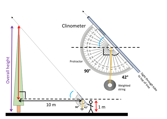
| What is the *overall* height of the tree to the closest metre?
| 1 | 1 | 1 | null | $$
1\,\mathrm{m} + 10\,\mathrm{m} \times \tan(90\degree -42\degree) = 12.1\,\mathrm{m}
$$
| An ecologist is using a clinometer to estimate the height (and therefore the biomass) of a tree. A clinometer is a tube attached to a protractor with a weighted string (see the diagram below), which can be used to measure angles between the ground and a distant point. The ecologist stands exactly $10 \, \mathrm{m}$ from the base of the tree on level ground and sights the top of the tree through the tube of the clinometer. The clinometer is held exactly $1 \, \mathrm{m}$ above the ground. The angle made by the weight and the tube of the clinometer is $42 ^\circ$. 

What is the *overall* height of the tree to the closest metre?
| 110 | 3 | 1 | 1 | 1 | 0 | 10 | 0 | 1 | An ecologist is using a clinometer to estimate the height and therefore the biomass of a tree. A clinometer is a tube attached to a protractor with a weighted string see the diagram below, which can be used to measure angles between the ground and a distant point. What is the overall height of the tree to the closest metre? | 3 |
0d36ee3e-25fd-49a8-9452-894589501cb0 | 0 | 4 | 0 | 19 | 6 | 1 | 5 | 0 | **(L7/8)**: For each of the following sets of simultaneous equations, determine if there is:
1. A unique solution
2. No solutions
3. An infinity of solutions
| $$
\begin{aligned}
x+y+z&=6\, ,\\
2x+y-z&=3\, ,\\
x+y&=4\, .
\end{aligned}
$$
\n$$
\begin{aligned}
x+y+z&=6\, ,\\
2x+y-z&=3\, ,\\
4x+3y+z&=1\, .
\end{aligned}
$$
\n$$
\begin{aligned}
x+y+z&=6\, ,\\
2x+y-z&=3\, ,\\
2x+2y+2z&=12\, .
\end{aligned}
$$
\n$$
\begin{aligned}
-x+2y-2z&=1, \\
4x-y+6z&=2\, ,\\
2x+3y+2z&=4\, ,\\
\end{aligned}
$$
| 4 | 0.333333 | 3 | Refer to **section 2.7**: what are the Cramer's Rule conditions for unique solutions, no solutions or an infinity of solutions? **Note:** In some cases, you *may* be able to deduce the type of solution by inspecting the simultaneous equations: are the planes independent?
***
Start by evaluating $\Delta$ (to speed this up, use determinant properties from **section 2.2**)...
***
... If $\Delta=0$, you must now check for unique solutions, or an infinity of solutions. 
***
Evaluate one of $\Delta_{1,2 ~\text{or} ~3}$. If you find that any are non-zero, this indicates no solutions.
***
For an infinity of solutions, each of $\Delta_{1,2~\text{and}~3}$ must be zero.
\nRefer to **section 2.7**: what are the Cramer's Rule conditions for unique solutions, no solutions or an infinity of solutions? **Note:** In some cases, you *may* be able to deduce the type of solution by inspecting the simultaneous equations: are the planes independent?
***
Start by evaluating $\Delta$ (to speed this up, use determinant properties from **section 2.2**)...
***
... If $\Delta=0$, you must now check for unique solutions, or an infinity of solutions. 
***
Evaluate one of $\Delta_{1,2 ~\text{or} ~3}$. If you find that any are non-zero, this indicates no solutions.
***
For an infinity of solutions, each of $\Delta_{1,2~\text{and}~3}$ must be zero.
| (**Section 2.8**): We start by evaluating $\Delta$. If $\Delta\ne0$, there are unique solutions. If $\Delta=0$, we check for the other two cases:
* For no solutions, *one of* $\Delta_{1,2~\text{or}~3}$ is non-zero. 
* For an infinity of solutions, *all of* $\Delta_{1,2~\text{and}~3}$ must be zero. 
***
Evaluating $\Delta$, using determinant properties to simplify the evaluation:
***
$$
\Delta \ =
\begin{vmatrix} \ 1 &\ 1 &\ 1\\ 2 & 1 & -1\\ 1 & 1 & 0 \end{vmatrix} =
-\begin{vmatrix} \ 1 & 1 & 0\\ 2 & 1 & -1\\ 1 & 1 & 1 \end{vmatrix} =
-\begin{vmatrix} \ 1 & 0 & 0\\ 2 & -1 & -1\\ 1 & 0 & 1 \end{vmatrix} \
$$
* First, swapped R1 and R3.
* Then, subtracted C1 from C2. 
Reducing this to a 2$\times$2 determinant:
***
$$
=\
-\begin{vmatrix} -1 & -1\\ 0 & 1 \end{vmatrix} = 1
$$
$\Delta\ne0\implies$**Unique solutions**. 
\n(**Section 2.8**): We start by evaluating $\Delta$. If $\Delta\ne0$, there are unique solutions. If $\Delta=0$, we check for the other two cases:
* For no solutions, *one of* $\Delta_{1,2~\text{or}~3}$ is non-zero. 
* For an infinity of solutions, *all of* $\Delta_{1,2~\text{and}~3}$ must be zero. 
***
Evaluating $\Delta$, using determinant properties to simplify the evaluation:
***
$$
\Delta \ =
\begin{vmatrix} \ 1 &\ 1 &\ 1\\ 2 & 1 & -1\\ 4 & 3 & 1 \end{vmatrix} =
\begin{vmatrix} 1 & 0 & 0\\ 2 & -1 & -3\\ 4 & -1 & -3 \end{vmatrix} =\ \begin{vmatrix} \ 1 & 3 \\ \ 1 & 3 \end{vmatrix} =0\
$$
* Subtracted C1 from C2 and C3.
***
$\Delta=0\implies$No unique solutions. Now we must check for no solutions or an infinity of solutions. We start by choosing any of $\Delta_{1,2,~\text{or}~3}$ to evaluate, e.g. $\Delta_3$:
***
$$
\Delta _{3} \ =\begin{vmatrix} \ 1 &\ 1 &\ 6\\ 2 & 1 & 3\\ 4 & 3 & 1 \end{vmatrix} = \begin{vmatrix} 1 & 0 & 0\\ 2 & -1 & -9\\ 4 & -1 & -23 \end{vmatrix} =\
\begin{vmatrix} 1 & 9\\ 1 & 23 \end{vmatrix} =14
$$
* Subtracted C1 from C2, and 6$\times$C1 from C3. 
We have found a single determinant that in non-zero, so there are **no solutions** to this system of equations.
\n(**Section 2.8**): We start by evaluating $\Delta$. If $\Delta\ne0$, there are unique solutions. If $\Delta=0$, we check for the other two cases:
* For no solutions, *one of* $\Delta_{1,2~\text{or}~3}$ is non-zero. 
* For an infinity of solutions, *all of* $\Delta_{1,2~\text{and}~3}$ must be zero.
**Note:** In this question, it is possible to see the type of solution by inspecting the equations: are the planes linearly independent? (the methodology behind this is discussed at the end)
***
Evaluating $\Delta$, using determinant properties to simplify the evaluation:
***
$$
\Delta \ =
\begin{vmatrix}\ 1 &\ 1 & 1\\ 2 & 1 & -1\\ 2 & 2 & 2 \end{vmatrix} =
\begin{vmatrix}\ 1 &\ 0 & 0\\ 2 & 1 & -1\\ 2 & 0 & 0 \end{vmatrix} =0
$$
* We notice that R3 is simply 2$\times$R1, and so we could multiply R3 so that R1=R3. If two determinant row/columns are equivalent, the determinant evaluates to 0. 
***
$\Delta=0\implies$No unique solutions. Now we must check for no solutions or an infinity of solutions. We start by choosing any of $\Delta_{1,2,~\text{or}~3}$ to evaluate.
***
$$
\Delta _{1} \ =
\begin{vmatrix} 6 & 1 & 1\\ 3 & 1 & -1\\ 12 & 2 & 2 \end{vmatrix} = 0 ,
\qquad
\Delta _{2} \ =
\begin{vmatrix}\ 1 &\ 1 & 1\\ 2 & 1 & -1\\ 2 & 2 & 2 \end{vmatrix} = 0,
\qquad
\Delta _{3} \ =
\begin{vmatrix}\ 1 &\ 1 & 1\\ 2 & 1 & -1\\ 2 & 2 & 2 \end{vmatrix} = 0
$$
* In each case, R3 is a multiple of R1, so as before, they immediately evaluate to 0. 
***
Since each of $\Delta_{1,2 ~ \text{and} ~ 3}$ is zero, there are an **infinity** **of solutions**. Indeed, we could have spotted initially that the bottom equation is multiple of top, so there are only two independent equations for three unknowns $ \rightarrow $ not enough to have a unique solution. Hence there will just be an intersection between the two independent planes.
\n(**Section 2.8**): We start by evaluating $\Delta$. If $\Delta\ne0$, there are unique solutions. If $\Delta=0$, we check for the other two cases:
* For no solutions, *one of* $\Delta_{1,2~\text{or}~3}$ is non-zero. 
* For an infinity of solutions, *all of* $\Delta_{1,2~\text{and}~3}$ must be zero. 
***
Evaluating $\Delta$, using determinant properties to simplify the evaluation:
***
$$
\Delta \ =\begin{vmatrix} -1 & 2 & -2\\ 4 & -1 & 6\\ 2 & 3 & 2 \end{vmatrix} =
\begin{vmatrix} -1 & 0 & 0\\ 4 & 7 & -2\\ 2 & 7 & -2 \end{vmatrix} \ =\
\begin{vmatrix} 7 & -2\\ 7 & -2 \end{vmatrix} =0
$$
* Added 2$\times$C1 to C2, and subtracted 2$\times$C1 from C3. 
***
$\Delta=0\implies$No unique solutions. Now we must check for no solutions or an infinity of solutions. We start by choosing any of $\Delta_{1,2,~\text{or}~3}$ to evaluate.
***
$$
\begin{aligned}
&
\Delta _{1} \ =
\begin{vmatrix} 1 & 2 & -2\\ 2 & -1 & 6\\ 4 & 3 & 2 \end{vmatrix} =
\begin{vmatrix} 1 & 0 & 0\\ 2 & -5 & 10\\ 4 & -5 & 10 \end{vmatrix} = 0,\\
\end{aligned}
$$
* Subtracted 2$\times$C1 from C2, and added 2$\times$C1 to C3.
* Observe that the resulting 2$\times$2 determinant has equal rows/columns, and so evaluates to 0.
***
$$
\begin{aligned}
&
\Delta _{2} \ =
\begin{vmatrix} -1 & 1 & -2\\ 4 & 2 & 6\\ 2 & 4 & 2 \end{vmatrix} =
\begin{vmatrix} -1 & 0 & 0\\ 4 & 6 & -2\\ 2 & 6 & -2 \end{vmatrix} =
0\\
\end{aligned}
$$
* Added C1 to C2, and subtracted 2$\times$C1 from C3.
* Observe that the resulting 2$\times$2 determinant has equal rows/columns, and so evaluates to 0.
***
$$
\begin{aligned}
&
\Delta _{3} \ =\begin{vmatrix} -1 & 2 & 1\\ 4 & -1 & 2\\ 2 & 3 & 4 \end{vmatrix} =
\begin{vmatrix} -1 & 0 & 0\\ 4 & 7 & 6\\ 2 & 7 & 6 \end{vmatrix} \ =\
\begin{vmatrix} 7 & 6\\ 7 & 6 \end{vmatrix} =0
\end{aligned}
$$
* Added 2$\times$C1 to C2, and added C1 to C3.
* Observe that the resulting 2$\times$2 determinant has equal rows/columns, and so evaluates to 0.
***
Since each of $\Delta_{1,2 ~ \text{and} ~ 3}$ is zero, there are an **infinity** **of solutions**. This was not so obvious from the simultaneous equations. 
| **(L7/8)**: For each of the following sets of simultaneous equations, determine if there is:
1. A unique solution
2. No solutions
3. An infinity of solutions
$$
\begin{aligned}
x+y+z&=6\, ,\\
2x+y-z&=3\, ,\\
x+y&=4\, .
\end{aligned}
$$
\n$$
\begin{aligned}
x+y+z&=6\, ,\\
2x+y-z&=3\, ,\\
4x+3y+z&=1\, .
\end{aligned}
$$
\n$$
\begin{aligned}
x+y+z&=6\, ,\\
2x+y-z&=3\, ,\\
2x+2y+2z&=12\, .
\end{aligned}
$$
\n$$
\begin{aligned}
-x+2y-2z&=1, \\
4x-y+6z&=2\, ,\\
2x+3y+2z&=4\, ,\\
\end{aligned}
$$
| 33 | 4 | 57 | 57 | 650 | 16 | 7 | 4 | 0 | L7/8: For each of the following sets of simultaneous equations, determine if there is: 1. \end{aligned} $ $ \begin{aligned} x+y+z&=6\, ,\\ 2x+y-z&=3\, ,\\ 4x+3y+z&=1\, . \end{aligned} $ $ \begin{aligned} x+y+z&=6\, ,\\ 2x+y-z&=3\, ,\\ 2x+2y+2z&=12\, . \end{aligned} $ $ \begin{aligned} -x+2y-2z&=1, \\ 4x-y+6z&=2\, ,\\ 2x+3y+2z&=4\, ,\\ \end{aligned} $ | 4 |
0d4b9dc3-b242-493c-982a-e08fefe374f5 | 0 | 0 | 1 | 11 | 4 | 2 | 6 | 4 | Consider a counterflow heat exchanger in which the fluids on the hot and cold sides have inlet temperatures $T_\mathrm{hi}$ and $T_\mathrm{ci}$ respectively, while the temperature of the environment is $T_0$. The fluids can be taken to be the same gas on each side, assumed to behave as a perfect gas with constant-pressure specific heat $c_\mathrm{p}$. The mass flow rate $\dot{m}$ is the same on each side, so that the temperature difference $\Delta T$ between the hot and cold sides is constant throughout the heat exchanger. Heat loss from the heat exchanger casing and frictional pressure drops can be neglected. Show that the exergy destruction $\dot{B}_\mathrm{destroyed}$ or irreversibility $\dot{I}$ can be expressed in dimensionless form by:
| $\frac{\dot{B}_\mathrm{destroyed}}{\dot{m}c_\mathrm{p}T_0} = \frac{\dot{I}}{\dot{m}c_\mathrm{p}T_0} = \mathrm{ln}(1+K_1\Delta T + K_2(\Delta T)^2)$
  
where
  
$K_1 = \frac{T_\mathrm{hi}- T_\mathrm{ci}}{T_\mathrm{hi}T_\mathrm{ci}}$
  
and 
  
$K_2 = -\frac{1}{T_\mathrm{hi}T_\mathrm{ci}}$
| 1 | 1 | 2 | null | It can be helpful to draw a diagram of the heat exchanger:
***
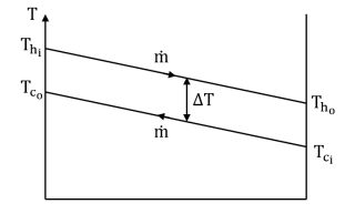
***
$\dot{B}_\mathrm{destroyed} = \dot{I} = T_0\dot{S}_\mathrm{gen}$
***
where $\dot{S}_\mathrm{gen} = \dot{S_2}-\dot{S_1}$
***
For a perfect gas:
  
$\dot{S_2}-\dot{S_1} = \dot{m}[c_\mathrm{p} \mathrm{ln}(\frac{T_2}{T_1})+R\mathrm{ln}(\frac{P_2}{P_1})]$
***
Since there is no pressure drop, $P_2 = P_1$ and the above expression simplifies to:
***
$\dot{S_2}-\dot{S_1} = \dot{m}c_\mathrm{p} \mathrm{ln}(\frac{T_2}{T_1})$
***
For both streams together:
  
$\dot{S_2}-\dot{S_1} = \dot{m}c_\mathrm{p}[\mathrm{ln}(\frac{T_\mathrm{h_o}}{T_\mathrm{h_i}}) + \mathrm{ln}(\frac{T_\mathrm{c_o}}{T_\mathrm{c_i}})]$
***
$\dot{S_2}-\dot{S_1} = \dot{m}c_\mathrm{p}\mathrm{ln}(\frac{T_\mathrm{h_o}T_\mathrm{c_o}}{T_\mathrm{h_i}T_\mathrm{c_i}})$
***
$T_\mathrm{h_o} = T_\mathrm{c_i} + \Delta T$
   
$T_\mathrm{c_o} = T_\mathrm{h_i} - \Delta T$
***
Hence:
  
$\dot{S_2}-\dot{S_1} = \dot{m}c_\mathrm{p}\mathrm{ln}(\frac{(T_\mathrm{c_i} + \Delta T)(T_\mathrm{h_i} - \Delta T)}{T_\mathrm{h_i}T_\mathrm{c_i}})$
***
Expanding the numerator:
  
$\dot{S_2}-\dot{S_1} = \dot{m}c_\mathrm{p}\mathrm{ln}(\frac{T_\mathrm{c_i}T_\mathrm{h_i} + \Delta T(T_\mathrm{h_i} -T_\mathrm{c_i}) - (\Delta T)^2}{T_\mathrm{h_i}T_\mathrm{c_i}})$
***
Simplifiying:
  
$\dot{S_2}-\dot{S_1} = \dot{m}c_\mathrm{p}\mathrm{ln}(1 + K_1\Delta T + K_2 (\Delta T)^2)$
***
Therefore:
  
$\dot{B}_\mathrm{destroyed} = \dot{I} = T_0\dot{m}c_\mathrm{p}\mathrm{ln}(1 + K_1\Delta T + K_2 (\Delta T)^2)$
***
Dividing by $\dot{m}c_\mathrm{p}T_0$:
  
$\frac{\dot{B}_\mathrm{destroyed}}{\dot{m}c_\mathrm{p}T_0} = \frac{\dot{I}}{\dot{m}c_\mathrm{p}T_0} = \mathrm{ln}(1+K_1\Delta T + K_2(\Delta T)^2)$
| Consider a counterflow heat exchanger in which the fluids on the hot and cold sides have inlet temperatures $T_\mathrm{hi}$ and $T_\mathrm{ci}$ respectively, while the temperature of the environment is $T_0$. The fluids can be taken to be the same gas on each side, assumed to behave as a perfect gas with constant-pressure specific heat $c_\mathrm{p}$. The mass flow rate $\dot{m}$ is the same on each side, so that the temperature difference $\Delta T$ between the hot and cold sides is constant throughout the heat exchanger. Heat loss from the heat exchanger casing and frictional pressure drops can be neglected. Show that the exergy destruction $\dot{B}_\mathrm{destroyed}$ or irreversibility $\dot{I}$ can be expressed in dimensionless form by:
$\frac{\dot{B}_\mathrm{destroyed}}{\dot{m}c_\mathrm{p}T_0} = \frac{\dot{I}}{\dot{m}c_\mathrm{p}T_0} = \mathrm{ln}(1+K_1\Delta T + K_2(\Delta T)^2)$
  
where
  
$K_1 = \frac{T_\mathrm{hi}- T_\mathrm{ci}}{T_\mathrm{hi}T_\mathrm{ci}}$
  
and 
  
$K_2 = -\frac{1}{T_\mathrm{hi}T_\mathrm{ci}}$
| 125 | 11 | 15 | 15 | 81 | 0 | 9 | 3 | 0 | Consider a counterflow heat exchanger in which the fluids on the hot and cold sides have inlet temperatures $T_\mathrm{hi}$ and $T_\mathrm{ci}$ respectively, while the temperature of the environment is $T_0$. The fluids can be taken to be the same gas on each side, assumed to behave as a perfect gas with constant-pressure specific heat $c_\mathrm{p}$. Show that the exergy destruction $\dot{B}_\mathrm{destroyed}$ or irreversibility $\dot{I}$ can be expressed in dimensionless form by: $\frac{\dot{B}_\mathrm{destroyed}}{\dot{m}c_\mathrm{p}T_0} = \frac{\dot{I}}{\dot{m}c_\mathrm{p}T_0} = \mathrm{ln}(1+K_1\Delta T + K_2(\Delta T)^2)$ where $K_1 = \frac{T_\mathrm{hi}- T_\mathrm{ci}}{T_\mathrm{hi}T_\mathrm{ci}}$ and $T_\mathrm{ci}$0 | 3 |
0d81759e-b284-40f7-854b-fce603b34a62 | 1 | 0 | 0 | 13 | 4 | 2 | 4 | 0 | A wheel is rolling along a horizontal path towards a step which lies across its path.
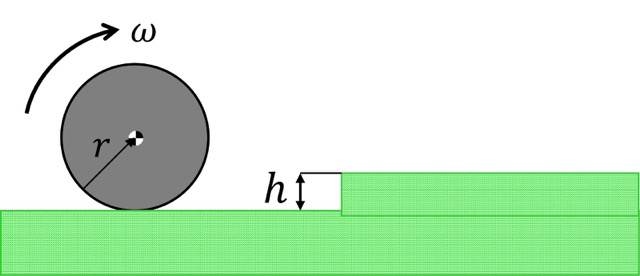
The wheel, of radius $r = 0.5~\mathrm{m}$ and radius of gyration $k = 0.4~\mathrm{m}$ about its centre, rolls with angular velocity $\omega=2~\mathrm{rad/s}$ along a horizontal path towards a step of height $h = 0.2~ \mathrm{m}$ ($ < r $).
| Find the angular velocity $\dot{\theta}_2$ of the wheel at the instant when it leaves the path and starts to mount the step. Assume no slip and no rebound from the step.
*(Take rotation in the clockwise direction to be positive)*
| 1 | 0.666667 | 3 | Let’s take angular momentum about a fixed point to make our lives easier and apply the conservation of momentum principle. What would be a suitable point? 
***
The top tip of the step serves this purpose very well in this case for example. 
Remember that the total angular momentum about a point is the sum of the angular momentum of the moving body around its own centre of gravity and the moment produced by its linear momentum about the chosen point –in this case it would be the angular momentum of the wheel around its centre and the moment of its linear momentum about the tip of the step (momentum times the perpendicular distance).
***
After impact, the wheel spins about itself as well as the step (consider the tangential velocity here), so the angular momentum equation about the step tip will have two respective expressions. The conservation of momentum method will help you find an expression for the angular velocity after impact. You’ll find it easier to first write your expressions of angular momentum in terms of linear velocities, the mass of the wheel and the mass moment of inertia about its centre of gravity.
***
After rearranging to find an expression for the angular velocity after impact, substitute in the variables given to you in the questions as the required answer is only in terms of the variables provided (i.e. the angular velocity before impact, the radius of the wheel $r$, the radius of gyration of the wheel $k$ about its centre and the height of the step $h$).
| Free body diagram and kinematic diagram:
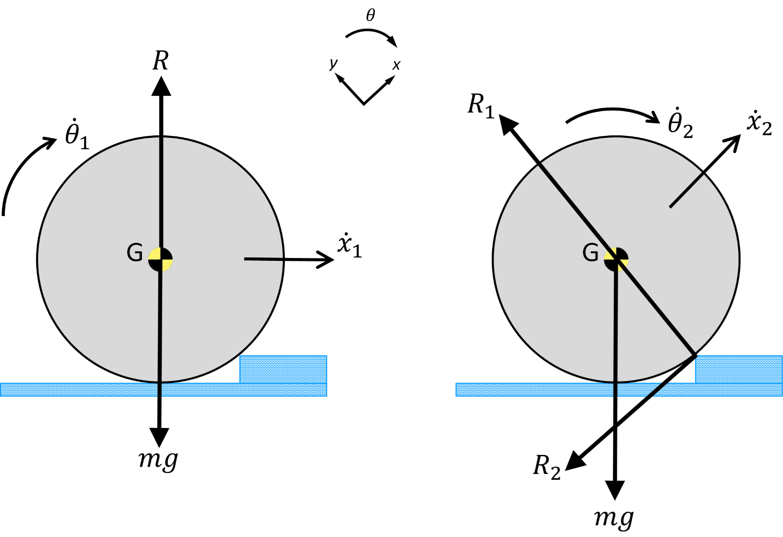
***
Starting with the equation for angular momentum about a general point:
$$
\begin{aligned}
H_O=I_G\dot{\theta}+m{\dot{x}}_G\left(y_G-y_O\right)-m{\dot{y}}_G\left(x_G-x_O\right)
\end{aligned}
$$
***
Consider the angular momentum at point O before the impact:
$$
\begin{aligned}
H_{O,1}=I_G{\dot{\theta}}_1+m{\dot{x}}_1\left(r-h\right)~~\mathrm{(Equation~1)}
\end{aligned}
$$
***
Consider the angular momentum at point O after the impact:
$$
\begin{aligned}
H_{O,2}=I_G{\dot{\theta}}_2+m{\dot{x}}_2r~~\mathrm{(Equation~2)}
\end{aligned}
$$
***
Applying conservation of momentum by combining Equations 1 and 2:
$$
\begin{aligned}
I_G{\dot{\theta}}_1+m{\dot{x}}_1\left(r-h\right)=I_G{\dot{\theta}}_2+m{\dot{x}}_2r~~\mathrm{(Equation~3)}
\end{aligned}
$$
***
But there is no slip so:
$$
\begin{aligned}
\dot{x}=r\dot{\theta}
\end{aligned}
$$
***
And the moment of inertia is given by:
$$
\begin{aligned}
I_G=mk^2
\end{aligned}
$$
***
Equation 3 can therefore be rewritten as:
$$
\begin{aligned}
\left(mk^2\right){\dot{\theta}}_1+m\left(r{\dot{\theta}}_1\right)\left(r-h\right)={\left(mk^2\right)\dot{\theta}}_2+m\left(r{\dot{\theta}}_2\right)r
\end{aligned}
$$
***
Rearranging for ${\dot{\theta}}_2$:
$$
\begin{aligned}
{\dot{\theta}}_2={\dot{\theta}}_1\frac{\left(k^2+r\left(r-h\right)\right)}{\left(r^2+k^2\right)}
\end{aligned}
$$
***
Substituting the values of the parameters gives:
$$
\begin{aligned}
{\dot{\theta}}_2=2\times\frac{\left({0.4}^2+0.5\times\left(0.5-0.2\right)\right)}{\left({0.5}^2+{0.4}^2\right)}
\end{aligned}
$$
$$
{\dot{\theta}}_2=1.51~\mathrm{rad/s}
$$
| A wheel is rolling along a horizontal path towards a step which lies across its path.

The wheel, of radius $r = 0.5~\mathrm{m}$ and radius of gyration $k = 0.4~\mathrm{m}$ about its centre, rolls with angular velocity $\omega=2~\mathrm{rad/s}$ along a horizontal path towards a step of height $h = 0.2~ \mathrm{m}$ ($ < r $).
Find the angular velocity $\dot{\theta}_2$ of the wheel at the instant when it leaves the path and starts to mount the step. Assume no slip and no rebound from the step.
*(Take rotation in the clockwise direction to be positive)*
| 88 | 6 | 11 | 11 | 99 | 3 | 40 | 1 | 1 | Find the angular velocity $\dot{\theta}_2$ of the wheel at the instant when it leaves the path and starts to mount the step. Assume no slip and no rebound from the step. Take rotation in the clockwise direction to be positive | 3 |
0da53862-6330-4f62-a563-840b35c837dd | 2 | 0 | 0 | 14 | 4 | 2 | 4 | 3 | Tests on a model propeller in a wind tunnel at sea level (air density $\rho = 1.2\,\mathrm{kg/m}^3$) gave the following results for the thrust at a number of forward velocities.
  
$$
\begin{array} {c|ccccc} \mathrm{U (m/s)}&\mathrm{0}&\mathrm{10}&\mathrm{15}&\mathrm{20}&\mathrm{30}\\ \hline \mathrm{Thrust (N)}&\mathrm{300}&\mathrm{278}&\mathrm{245}&\mathrm{211}&\mathrm{100} \end{array}
$$
  
The propeller diameter was $0.8,\mathrm{m}$ and it was spun at $2000,\mathrm{rpm}$.
| Using dimensional analysis find the non-dimensional parameters which govern this observed behavior.\nUsing experimental data given in the table, find the thrust generated by a geometrically similar propeller of diameter $3\,\mathrm{m}$, spinning at $1500\,\mathrm{rpm}$ at a forward velocity of $45\,\mathrm{m/s}$, while operating at an altitude where the density is half that at sea level. You may interpolate from tabulated values. | 2 | 0.5 | 2 | \n | \n | Tests on a model propeller in a wind tunnel at sea level (air density $\rho = 1.2\,\mathrm{kg/m}^3$) gave the following results for the thrust at a number of forward velocities.
  
$$
\begin{array} {c|ccccc} \mathrm{U (m/s)}&\mathrm{0}&\mathrm{10}&\mathrm{15}&\mathrm{20}&\mathrm{30}\\ \hline \mathrm{Thrust (N)}&\mathrm{300}&\mathrm{278}&\mathrm{245}&\mathrm{211}&\mathrm{100} \end{array}
$$
  
The propeller diameter was $0.8,\mathrm{m}$ and it was spun at $2000,\mathrm{rpm}$.
Using dimensional analysis find the non-dimensional parameters which govern this observed behavior.\nUsing experimental data given in the table, find the thrust generated by a geometrically similar propeller of diameter $3\,\mathrm{m}$, spinning at $1500\,\mathrm{rpm}$ at a forward velocity of $45\,\mathrm{m/s}$, while operating at an altitude where the density is half that at sea level. You may interpolate from tabulated values. | 105 | 7 | 0 | 0 | 1 | 0 | 61 | 3 | 0 | Tests on a model propeller in a wind tunnel at sea level air density $\rho = 1.2\,\mathrm{kg/m}^3$ gave the following results for the thrust at a number of forward velocities. Using dimensional analysis find the non-dimensional parameters which govern this observed behavior. Using experimental data given in the table, find the thrust generated by a geometrically similar propeller of diameter $3\,\mathrm{m}$, spinning at $1500\,\mathrm{rpm}$ at a forward velocity of $45\,\mathrm{m/s}$, while operating at an altitude where the density is half that at sea level. | 3 |
0df0dd8e-3185-427a-9f46-f4e28cddca81 | 1 | 0 | 0 | 10 | 4 | 2 | 8 | 2 | The creep rupture properties of Nimonic 105 are shown in the figure below. Using this figure, estimate the maximum operating temperature of a gas turbine blade made out of this material which is to withstand a stress of $150\text{ MPa}$ for a duration of $10,000$ hours. 
   
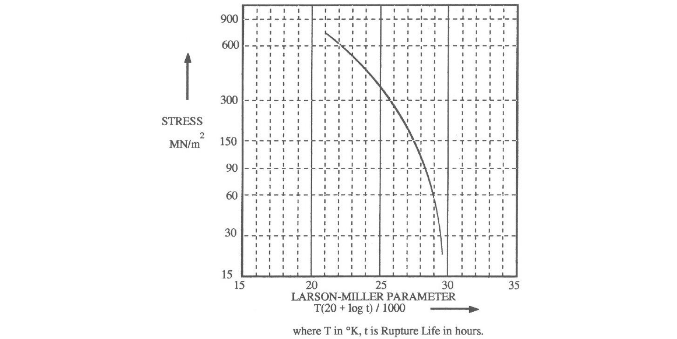
$$
\footnotesize
\text{Figure Q4.3: Graph of Larson-Miller Parameter vs. Stress}
$$
| What would be the new design life if the engine rate $40^\circ\text{C}$ hotter?
| 1 | 0.666667 | 2 | null | Using the following equation for the Larson-Miller Parameter:
   
$$
P_{LM}=T(\log t_r+C)
$$
   
Where $T$ is the temperature, $t_r$ is the time to rupture, and $C=T(20+\log t)$.
   
***
Using values read from the graph at $150\text{ MPa}$:
   
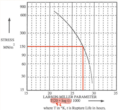
$$
\footnotesize
\text{Figure Q4.3.1: Annotated Larson-Miller Parameter vs. Stress graph.}
$$
   
***
And then substituting numbers into the earlier equation:
   
$$
27.5\times10^3=T(\log10,000+20)\\
~\\
T=1146\text{ K}=873\degree\text{C}
$$
   
***
Increasing $T$ by $40\degree \text{C}$ and then substituting back into the equation to find a new value for $t_r$.
   
$$
T=913\degree\text{C}=1186\text{ K}
$$
   
$$
27.5\times10^3=1186(\log t_r+20)\\ ~\\
t_r=1538\text{ hours}\approx\boxed{1500\text{ hours}}
$$
| The creep rupture properties of Nimonic 105 are shown in the figure below. Using this figure, estimate the maximum operating temperature of a gas turbine blade made out of this material which is to withstand a stress of $150\text{ MPa}$ for a duration of $10,000$ hours. 
   

$$
\footnotesize
\text{Figure Q4.3: Graph of Larson-Miller Parameter vs. Stress}
$$
What would be the new design life if the engine rate $40^\circ\text{C}$ hotter?
| 62 | 4 | 12 | 12 | 85 | 0 | 13 | 1 | 1 | Using this figure, estimate the maximum operating temperature of a gas turbine blade made out of this material which is to withstand a stress of $150\text{ MPa}$ for a duration of $10,000$ hours. Stress} $ What would be the new design life if the engine rate $40^\circ\text{C}$ hotter? | 2 |
0ea1717d-dcaa-4eec-a76f-2f7a350b1878 | 0 | 1 | 0 | 2 | 1 | 2 | 0 | 13 | Select all of the features that describe a turbulent flow.
| Select all of the features that describe a turbulent flow.
| 1 | 0.333333 | 0 | null | null | Select all of the features that describe a turbulent flow.
| 10 | 0 | 0 | 0 | 0 | 0 | 10 | 0 | 0 | Select all of the features that describe a turbulent flow. | 1 |
0f457acf-716d-416e-924b-091158ac4995 | 3 | 0 | 0 | 19 | 6 | 1 | 9 | 4 | A particle starts at position $\vec{r}_{0}=(0, 1, 0)$ with a velocity $\vec{v} = (2, 1, 3)$. It collides with a wall whose position is given by the equation $x+y+z = 4$. (You may assume throughout this question that all physical quantities are given in dimensionless units, and there are no external forces acting on the particle.)
| Give an expression for the trajectory of the particle before the collision. 
\nFind the position at which the particle strikes the wall. 
\nFind the velocity of the particle after the collision with the wall, assuming the collision is elastic.
| 3 | 0.666667 | 2 | $\vec{r}(t) = \vec{r}_0 + \vec{v}t$
\nYour goal is to find the intersection of the linear trajectory of the particle and the plane.
***
Express your trajectory equation from part (a) as $x=x(t),y=y(t),z=z(t)$. 
***
Insert these results into the equation of the plane and solve for the time of intersection.
***
Using this time, can you find the *point* of intersection?
\nDraw a diagram of the plane, and the incoming and outgoing trajectories. Add to your diagram the velocity components perpendicular and parallel to the plane.
***
Split the velocity *before* the collision into components parallel and perpendicular to the plane...
***
... The perpendicular component is the one parallel to the *normal* of the plane. 
***
Find this by computing the projection of $\vec{v}$ onto $\mathbf{\hat{n}}$.
***
After this, can you compute the parallel velocity component to the plane?
***
After the collision, which of the velocity components change, and how? Hence calculate the new velocity.
| $$
\vec{r}(t) = \vec{r}_0 + \vec{v}t=\begin{pmatrix}0\\1\\0\end{pmatrix}+\begin{pmatrix}2\\1\\3\end{pmatrix}t=\begin{pmatrix}2t\\1+1t\\3t\end{pmatrix}
$$
\nFrom part (a): $x=2 t, \quad y=1+t, \quad z=3 t$. Inserting this into the plane equation:
***
$$
\begin{array}{l l }
\text{in} \qquad x+y+z=4, \quad
& \Rightarrow 2 t+(1+t)+3 t=4 \\
&\Rightarrow \quad 6 t=3 \\
&\Rightarrow \quad t=1 / 2 \\
\end{array}
$$
***
Inserting this time into the trajectory of the particle yields the point of collision:
***
$$
\begin{array}{l}
\quad & \vec{r}_{\text {coll }}=\left(\begin{array}{l}
0 \\
1 \\
0
\end{array}\right)+\dfrac{1}{2}\left(\begin{array}{l}
2 \\
1 \\
3
\end{array}\right)=\left(\begin{array}{c}
1\\ 3 / 2 \\ 3 / 2
\end{array}\right)
\end{array}
$$
\n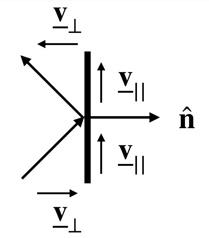
***
We start by expressing the velocity before the collision in terms of components *perpendicular* to the wall, and parallel to the wall.
***
The perpendicular component of the velocity is parallel to the normal vector $\mathbf{\underline{n}}=(1,1,1)$ of the plane. 
***
Hence, to find this component, we find the projection of $\vec{v}$ onto the normalised normal vector, using the dot product:
***
$$
\vec{n}=\left(\begin{array}{l}
1 \\ 1 \\ 1
\end{array}\right) \qquad \rightarrow \qquad \mathbf{\hat{n}}=\frac{1}{\sqrt{3}}\left(\begin{array}{l}
1 \\ 1 \\ 1
\end{array}\right)
$$
***
$$
\begin{align*}
\vec{v}_{\perp} \ =\ \frac{1}{\sqrt{3}}\left\{\left(\begin{array}{l}
1 \\ 1 \\ 1
\end{array}\right) \cdot\left(\begin{array}{l}
2 \\ 3 \\ 1
\end{array}\right)\right\}\frac{1}{\sqrt{3}}\left(\begin{array}{l}
1 \\ 1 \\ 1
\end{array}\right)\ = \
\frac{1}{3}\{6\} \cdot\left(\begin{array}{l}
1 \\
1 \\
1
\end{array}\right) \
=\ \left(\begin{array}{l}
2 \\ 2 \\ 2
\end{array}\right)
\end{align*}
$$
***
The parallel component to the plane before collision is found by negating the perpendicular component from $\vec{v}$ (see diagram):
***
$$
\vec{v}_{||}=\left(\begin{array}{l}
2 \\ 1 \\ 3
\end{array}\right)-\left(\begin{array}{l}
2 \\ 2 \\ 2
\end{array}\right)=\left(\begin{array}{c}
0 \\ -1 \\ 1
\end{array}\right)
$$
***
After the collision, the parallel component is unchanged, but the perpendicular component reverses. Therefore, 
$$
\vec{v}_{\perp}{^{\prime}}=\left(\begin{array}{l}
-2 \\ -2 \\ -2
\end{array}\right)
$$
Thus, the velocity vector after collision is:
***
$$
\vec{v}_{\text {after}}= \vec{v}_{\perp}{^{\prime}} +\vec{v}_{||}=\left(\begin{array}{c}
-2 \\
-2 \\
-2
\end{array}\right)+\left(\begin{array}{c}
0 \\
-1 \\
1
\end{array}\right) =\left(\begin{array}{c}
-2 \\
-3 \\
-1
\end{array}\right)
$$
| A particle starts at position $\vec{r}_{0}=(0, 1, 0)$ with a velocity $\vec{v} = (2, 1, 3)$. It collides with a wall whose position is given by the equation $x+y+z = 4$. (You may assume throughout this question that all physical quantities are given in dimensionless units, and there are no external forces acting on the particle.)
Give an expression for the trajectory of the particle before the collision. 
\nFind the position at which the particle strikes the wall. 
\nFind the velocity of the particle after the collision with the wall, assuming the collision is elastic.
| 89 | 3 | 12 | 12 | 144 | 4 | 39 | 0 | 0 | It collides with a wall whose position is given by the equation $x+y+z = 4$. You may assume throughout this question that all physical quantities are given in dimensionless units, and there are no external forces acting on the particle. Give an expression for the trajectory of the particle before the collision. Find the position at which the particle strikes the wall. Find the velocity of the particle after the collision with the wall, assuming the collision is elastic. | 5 |
10703359-bbd8-4c73-b85e-57c27e140d16 | 3 | 0 | 0 | 15 | 5 | 0 | 3 | 1 | If a population of cells is exposed to radioactive UTP labelled with $^{32}\mathrm{P}$ (a radioactive isotope of phosphorus), the mRNA being formed at that moment will be labelled. As the mRNA is degraded, the amount of labelled mRNA decreases exponentially with time (we will assume no radioactive uracil is recycled):
$$
L=L_{0}\cdot e^{-\lambda \cdot t}
$$
$$
\lambda = \frac{\ln{2}}{H}
$$
* $L$ Mass of labelled mRNA
<!---->
* $L_{0}$ Mass of labelled mRNA at beginning of experiment
<!---->
* $H$ Half-life of the mRNA (time it takes for half the mRNA to degrade)
<!---->
* $\lambda$ Decay constant
| Rearrange the left-hand equation for $\lambda$
\nCalculate the half-lives of histone H3 and fructose-*bis*-phosphatase mRNAs from the data below. How much longer lived is FBP mRNA than H3 mRNA?
| mRNA | Mass of labelled mRNA at $t=0 \,\mathrm{min}$ ($\mathrm{\mu g \cdot L^{-1}}$) | Mass of labelled mRNA at $t=180 \mathrm{min}$ ($\mathrm{\mu g \cdot L^{-1}}$) |
| :--------- | :---------------------------------------------------------------------------- | :---------------------------------------------------------------------------- |
| FBP | 1.00 | 0.812 |
| Histone H3 | 20.0 | 0.313 |
\nAfter messing about with all this radioactivity, you need to dispose of the radioactive waste. Given that the waste has an activity of $3360 \, \mathrm{Bq}$ (the Becquerel is the SI unit of radioactivity), and that $^{32}\mathrm{P}$ has a half-life of $14.28 \mathrm{days}$, how long would you need to wait until the activity has decayed to just $10 \, \mathrm{Bq}$?
| 3 | 1 | 1 | \n\n | $\lambda=\frac{-\ln{\frac{L}{L_0}}}{t}=\frac{\ln{L_0}-\ln{L}}{t}$
There are lots of other ways of writing this!
\nHalf-lives are $10$ and $0.5$
$10/0.5= 20$
| mRNA | Calculation | $H$ |
| :--------- | :---------------------------------------------------------------- | :---- |
| FBP | $H=\frac{\ln{2}}{\left(\frac{\ln{1}-\ln{0.812}}{180}\right)}=600$ | $10$ |
| Histone H3 | $H=\frac{\ln{2}}{\left(\frac{\ln{20}-\ln{0.313}}{180}\right)}=30$ | $0.5$ |
\n$$
P=P_0e^{-\left(\frac{\ln{2}}{H}\right)t}\
\newline
t=-\frac{\ln{\left(\frac{P}{P_0}\right)}}{\left(\frac{\ln{2}}{H}\right)}=-\frac{\ln{\left(\frac{10}{3360}\right)}}{\left(\frac{\ln{2}}{14.28}\right)}=120\,\mathrm{d}
$$
| If a population of cells is exposed to radioactive UTP labelled with $^{32}\mathrm{P}$ (a radioactive isotope of phosphorus), the mRNA being formed at that moment will be labelled. As the mRNA is degraded, the amount of labelled mRNA decreases exponentially with time (we will assume no radioactive uracil is recycled):
$$
L=L_{0}\cdot e^{-\lambda \cdot t}
$$
$$
\lambda = \frac{\ln{2}}{H}
$$
* $L$ Mass of labelled mRNA
<!---->
* $L_{0}$ Mass of labelled mRNA at beginning of experiment
<!---->
* $H$ Half-life of the mRNA (time it takes for half the mRNA to degrade)
<!---->
* $\lambda$ Decay constant
Rearrange the left-hand equation for $\lambda$
\nCalculate the half-lives of histone H3 and fructose-*bis*-phosphatase mRNAs from the data below. How much longer lived is FBP mRNA than H3 mRNA?
| mRNA | Mass of labelled mRNA at $t=0 \,\mathrm{min}$ ($\mathrm{\mu g \cdot L^{-1}}$) | Mass of labelled mRNA at $t=180 \mathrm{min}$ ($\mathrm{\mu g \cdot L^{-1}}$) |
| :--------- | :---------------------------------------------------------------------------- | :---------------------------------------------------------------------------- |
| FBP | 1.00 | 0.812 |
| Histone H3 | 20.0 | 0.313 |
\nAfter messing about with all this radioactivity, you need to dispose of the radioactive waste. Given that the waste has an activity of $3360 \, \mathrm{Bq}$ (the Becquerel is the SI unit of radioactivity), and that $^{32}\mathrm{P}$ has a half-life of $14.28 \mathrm{days}$, how long would you need to wait until the activity has decayed to just $10 \, \mathrm{Bq}$?
| 225 | 16 | 10 | 10 | 47 | 0 | 131 | 9 | 3 | As the mRNA is degraded, the amount of labelled mRNA decreases exponentially with time we will assume no radioactive uracil is recycled: $ L=L_{0}\cdot e^{-\lambda \cdot t} $ $ \lambda = \frac{\ln{2}}{H} $ $L$ Mass of labelled mRNA embedded $L_{0}$ Mass of labelled mRNA at beginning of experiment embedded $H$ Half-life of the mRNA time it takes for half the mRNA to degrade embedded $\lambda$ Decay constant Rearrange the left-hand equation for $\lambda$ Calculate the half-lives of histone H3 and fructose-bis-phosphatase mRNAs from the data below. How much longer lived is FBP mRNA than H3 mRNA? Given that the waste has an activity of $3360 \, \mathrm{Bq}$ the Becquerel is the SI unit of radioactivity, and that $^{32}\mathrm{P}$ has a half-life of $ L=L_{0}\cdot e^{-\lambda \cdot t} $0, how long would you need to wait until the activity has decayed to just $ L=L_{0}\cdot e^{-\lambda \cdot t} $1? | 3 |
10cb0c12-9685-4f7f-9bc4-fe7f3022a872 | 3 | 0 | 0 | 8 | 4 | 2 | 3 | 2 | Two strain gauges are fitted at $\pm45^{\circ}$ to the axis of a $75\text{ mm}$ diameter steel shaft. The shaft is rotating, and in addition to transmitting power, it is subjected to an unknown bending moment and a direct thrust. The readings of the gauges are recorded, and it is found that the maxima or minima values for each gauge occur at $180^{\circ}$ intervals of shaft rotation and are $-0.00060$ and $+0.00030$ for the two gauges at one instant, and $-0.00050$ and $+0.00040$ for the same gauges $180^{\circ}$ of rotation later. Assume that all the forces and moments are steady, i.e. they do not vary during each rotation of the shaft.
| Calculate the transmitted torque.
\nCalculate the applied bending moment.
\nCalculate the end thrust.
| 3 | 1 | 4 | \n\n | First draw a diagram of the problem:
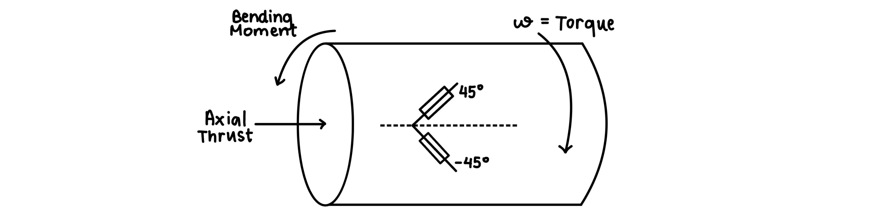  
The strain gauges readings pre rotation:
   
$$
e_{45}=-0.00060 \hspace{30pt} e_{-45}=+0.00030
$$
   
The strain gauge readings post rotation:
   
$$
e_{45}=-0.00050 \hspace{30pt} e_{-45}=+0.00040
$$
   
***
To calculate the transmitted torque, $\gamma_{\theta z}$ needs to be found.
   
***
Looking at both of the strain gauges and using equation 1 (note that the strain gauge values prior to rotation are used as it's best to find the shear stress that results from the torque alone.)
   
$$
\begin{align}
e_\text{n}=\frac{e_\theta+e_z}{2}+\frac{e_\theta-e_z}{2}\cos2\theta+\frac{\gamma_{\theta z}}{2}\sin2\theta
\end{align}
$$
   
***
@ $45\degree$:
$$
\begin{align*}
e_\text{45}&=\frac{e_\theta+e_z}{2}+\cancel{\frac{e_\theta-e_z}{2}\cos90}+\frac{\gamma_{\theta z}}{2}\cancel{\sin90}\\
\hspace{10pt}
\end{align*} \\
$$
$$
\begin{align}
-0.0006=\frac{e_\theta+e_z}{2}+\frac{\gamma_{\theta z}}{2}
\end{align}
$$
   
***
@ $-45\degree$:
$$
\begin{align*}
e_\text{45}&=\frac{e_\theta+e_z}{2}+\cancel{\frac{e_\theta-e_z}{2}\cos(-90)}+\frac{\gamma_{\theta z}}{2}\cancel{\sin(-90)}\\
\hspace{10pt}\\
\end{align*}
$$
$$
\begin{align}
0.0003&=\frac{e_\theta+e_z}{2}-\frac{\gamma_{\theta z}}{2}
\end{align}
$$
   
***
Using equation $(2)$ and $(3)$:
$$
\cancel{\frac{e_\theta+e_z}{2}}+\frac{\gamma_{\theta z}}{2}+0.0006=\cancel{\frac{e_\theta+e_z}{2}}-\frac{\gamma_{\theta z}}{2}-0.0003 \\
\hspace{10pt} \\
\gamma_{\theta z}=-0.0009
$$
   
***
To now find the transmitted torque, using equations from ME1-SAN:
   
$$
\tau=\frac{Tr}{J} \hspace{50pt} G=\frac{\tau}{\gamma}
$$
   
***
Combining the two equations, then solving for torque ($T$):
  
$$
\frac{Tr}{J}=G\gamma\\
\hspace{10pt} \\
\begin{aligned}
T&=\frac{G\gamma J}{r}\\
&=\left( \frac{79.6\times10^9\times-0.0009\times\frac{\pi}{32}(75\times10^{-3})^4}{(75\times10^{-3})}\right)\\
&=\boxed{-5.934\text{ kN}}
\end{aligned}
$$
   
Note that it is also possible to have the torque be positive as it depends on the chosen coordinate system.
\nTo find the bending moment, the following relationship needs to be used:
   
$$
\begin{align}
\sigma_{z, \text{ BM}}=\frac{My}{I} \hspace{30pt}\rightarrow \hspace{30pt}M=\frac{\sigma_{z, \text{ BM}}I}{y}
\end{align}
$$
   
***
First calculate the second moment of area ($I$) and the neutral axis ($y$). $\sigma_{z, \text{ BM}}$ is unknown.
   
$$
\begin{align}
I=\frac{\pi r^4}{4}=\frac{\pi(\frac{75}{2}\times10^{-3})^4}{4}=1.553\times10^{-6}\text{ m}^4
\end{align}
$$
   
$$
\begin{align}
y=r=0.0375 \text{ m}
\end{align}
$$
 
***
Looking at the strain in the normal direction as derived from part (a) for strain gauges that are $\pm\hspace{2pt}45\degree$
   
$$
\begin{align}
(\text{for strain gauge at }45\degree)\text{ }e_\text{n}&=\frac{e_z+e_\theta}{2}+\frac{\gamma_{\theta z}}{2}\\
(\text{for strain gauge at }-45\degree)\text{ }e_\text{n}&=\frac{e_z+e_\theta}{2}-\frac{\gamma_{\theta z}}{2}
\end{align}
$$
   
***
Then find the strain in the axial direction, making sure to include the axial strain as a result of the axial force applied to the shaft and the bending moment.
   
$$
\begin{align}
e_z=e_{AF}+e_{z,\text{ BM}}
\end{align}
$$
   
And find the hoop strain using the definition of Poisson's ratio:
   
$$
\begin{align}
\nu=-\frac{e_\theta}{e_z} \hspace{20pt} \rightarrow \hspace{20pt} e_\theta=-\nu e_z
\end{align}
$$
   
***
Substituting $e_\theta$ and $e_z$ into the equation for $e_\text{n}$:
   
$$
\begin{align}
e_\text{n}=\frac{(e_{AF}+e_{z,\text{BM}})-\nu(e_{AF}+e_{z,\text{BM}})}{2}\pm\frac{\gamma_{\theta z}}{2}
\end{align}
$$
   
***
First looking at the strain gauges prior to rotation:
   
$$
\begin{align}
-0.0006=\frac{1}{2}[(e_{AF}+e_{z,\text{BM}})(1-\nu)+\gamma_{\theta z}] \\
+0.0003=\frac{1}{2}[(e_{AF}+e_{z,\text{BM}})(1-\nu)-\gamma_{\theta z}]
\end{align}
$$
   
***
Subtract equation $(9)$ and equation $(10)$:
   
$$
\begin{align}
-0.0003=(e_{AF}+e_{z,\text{BM}})(1-\nu)
\end{align}
$$
   
***
Then substitute the values of the strain gauges post rotation, note the negative sign to accommodate the $180\degree$ rotation. 
   
$$
\begin{align}
-0.0005=\frac{1}{2}[(e_{AF}-e_{z,\text{BM}})(1-\nu)+\gamma_{\theta z}] \\
+0.0004=\frac{1}{2}[(e_{AF}-e_{z,\text{BM}})(1-\nu)-\gamma_{\theta z}]
\end{align}
$$
   
***
Subtract equation $(12)$ and $(13)$:
   
$$
\begin{align}
-0.0001=(e_{AF}-e_{z,\text{BM}})(1-\nu)
\end{align}
$$
   
***
Then add equations $(11)$ and $(14)$:
   
$$
\begin{align}
-0.0004=2(e_{AF})(1-\nu)
\end{align}
$$
   
***
Rearrange and solve for , using $\nu=0.3$:$e_{AF}$
$$
e_{AF}=-0.0002857
$$
   
***
Substitute $e_{AF}$ into equation $(11)$ to find $e_{z,\text{ BM}}$:
   
$$
\begin{align}
-0.0003&=(-0.002857+e_{z,\text{ BM}})(1-0.3)\\
e_{z,\text{ BM}}&=-0.0001429
\end{align}
$$
   
***
By definition, Young's Modulus is:
   
$$
\begin{align}
E=\frac{\sigma_{z,\text{ BM}}}{e_{z,\text{ BM}}} \hspace{30pt} \rightarrow \hspace{30pt} \sigma_{z,\text{ BM}}=E\times e_{z,\text{ BM}}
\end{align}
$$
   
As such, this can then be used to find the bending moment.
   
***
Going back to equation $(1)$ and substituting the values from $(2), (3),$ and $(17)$ to solve for the bending moment (where $E=207 \text{ GPa}$).
$$
M=\frac{E\times e_{z,\text{ BM}}\times I}{y}=\boxed{-1.225 \text{ kNm}}
$$
\nTo find the axial thrust, use the axial strain ($e_{AF}$) calculated in (b):
   
$$
F_{AF}=\sigma_{AF}\times{A}
$$
***
   
$$
\sigma_{AF}=-0.0002857\times207\times10^9=-59.14\text{ MPa} \\
\hspace{10pt}\\
F_{AF}=\frac{-59.14\times10^6}{\pi (37.5\times10^{-3})^2}=\boxed{-2.613\text{ kPa}}
$$
   
Note the negative sign as the shaft is in compression.
| Two strain gauges are fitted at $\pm45^{\circ}$ to the axis of a $75\text{ mm}$ diameter steel shaft. The shaft is rotating, and in addition to transmitting power, it is subjected to an unknown bending moment and a direct thrust. The readings of the gauges are recorded, and it is found that the maxima or minima values for each gauge occur at $180^{\circ}$ intervals of shaft rotation and are $-0.00060$ and $+0.00030$ for the two gauges at one instant, and $-0.00050$ and $+0.00040$ for the same gauges $180^{\circ}$ of rotation later. Assume that all the forces and moments are steady, i.e. they do not vary during each rotation of the shaft.
Calculate the transmitted torque.
\nCalculate the applied bending moment.
\nCalculate the end thrust.
| 122 | 8 | 58 | 58 | 491 | 0 | 13 | 0 | 0 | The readings of the gauges are recorded, and it is found that the maxima or minima values for each gauge occur at $180^{\circ}$ intervals of shaft rotation and are $-0.00060$ and $+0.00030$ for the two gauges at one instant, and $-0.00050$ and $+0.00040$ for the same gauges $180^{\circ}$ of rotation later. Assume that all the forces and moments are steady, i.e. Calculate the transmitted torque. Calculate the applied bending moment. Calculate the end thrust. | 5 |
117dcbfd-a250-41f3-8eeb-4be2993a67c3 | 0 | 1 | 0 | 15 | 5 | 0 | 1 | 1 | The binding of calcium ions to the signalling protein calmodulin can be modelled by the equation:
$$
\theta=\frac{C^{n}}{K_{d}+C^n}
$$
Where:
* $\theta$ is the fraction of calmodulin molecules bound to calcium 
* $C$ is the concentration of calcium
* $n$ is a constant, greater than zero
* $K_{d}$ is the apparent dissociation constant for the calmodulin/calcium complex; also a number greater than zero
| Consider a plot of $\theta$ ($Y$-axis) against $C$ ($X$-axis).
Which one of the following is true?
| 1 | 1 | 0 | null | As $C$ becomes very large compared to $K_d$, $θ$ tends to $C^{n} / ( C^{n} ) = 1 $
| The binding of calcium ions to the signalling protein calmodulin can be modelled by the equation:
$$
\theta=\frac{C^{n}}{K_{d}+C^n}
$$
Where:
* $\theta$ is the fraction of calmodulin molecules bound to calcium 
* $C$ is the concentration of calcium
* $n$ is a constant, greater than zero
* $K_{d}$ is the apparent dissociation constant for the calmodulin/calcium complex; also a number greater than zero
Consider a plot of $\theta$ ($Y$-axis) against $C$ ($X$-axis).
Which one of the following is true?
| 81 | 9 | 4 | 4 | 13 | 0 | 20 | 4 | 0 | Which one of the following is true? | 1 |
End of preview. Expand
in Dataset Viewer.
README.md exists but content is empty.
Use the Edit dataset card button to edit it.
- Downloads last month
- 0