
hexsha
stringlengths 40
40
| size
int64 6
14.9M
| ext
stringclasses 1
value | lang
stringclasses 1
value | max_stars_repo_path
stringlengths 6
260
| max_stars_repo_name
stringlengths 6
119
| max_stars_repo_head_hexsha
stringlengths 40
41
| max_stars_repo_licenses
sequence | max_stars_count
int64 1
191k
⌀ | max_stars_repo_stars_event_min_datetime
stringlengths 24
24
⌀ | max_stars_repo_stars_event_max_datetime
stringlengths 24
24
⌀ | max_issues_repo_path
stringlengths 6
260
| max_issues_repo_name
stringlengths 6
119
| max_issues_repo_head_hexsha
stringlengths 40
41
| max_issues_repo_licenses
sequence | max_issues_count
int64 1
67k
⌀ | max_issues_repo_issues_event_min_datetime
stringlengths 24
24
⌀ | max_issues_repo_issues_event_max_datetime
stringlengths 24
24
⌀ | max_forks_repo_path
stringlengths 6
260
| max_forks_repo_name
stringlengths 6
119
| max_forks_repo_head_hexsha
stringlengths 40
41
| max_forks_repo_licenses
sequence | max_forks_count
int64 1
105k
⌀ | max_forks_repo_forks_event_min_datetime
stringlengths 24
24
⌀ | max_forks_repo_forks_event_max_datetime
stringlengths 24
24
⌀ | avg_line_length
float64 2
1.04M
| max_line_length
int64 2
11.2M
| alphanum_fraction
float64 0
1
| cells
sequence | cell_types
sequence | cell_type_groups
sequence |
|---|---|---|---|---|---|---|---|---|---|---|---|---|---|---|---|---|---|---|---|---|---|---|---|---|---|---|---|---|---|---|
d0000eb66b25d89c2d8a5d46ce7f89d88ad58f91
| 14,725
|
ipynb
|
Jupyter Notebook
|
Lectures/09_StrainGage.ipynb
|
eiriniflorou/GWU-MAE3120_2022
|
52cd589c4cfcb0dda357c326cc60c2951cedca3b
|
[
"BSD-3-Clause"
] | 5
|
2022-01-11T17:38:12.000Z
|
2022-02-05T05:02:50.000Z
|
Lectures/09_StrainGage.ipynb
|
eiriniflorou/GWU-MAE3120_2022
|
52cd589c4cfcb0dda357c326cc60c2951cedca3b
|
[
"BSD-3-Clause"
] | null | null | null |
Lectures/09_StrainGage.ipynb
|
eiriniflorou/GWU-MAE3120_2022
|
52cd589c4cfcb0dda357c326cc60c2951cedca3b
|
[
"BSD-3-Clause"
] | 9
|
2022-01-13T17:55:14.000Z
|
2022-03-24T14:41:03.000Z
| 38.955026
| 518
| 0.584652
|
[
[
[
"# 09 Strain Gage\n\nThis is one of the most commonly used sensor. It is used in many transducers. Its fundamental operating principle is fairly easy to understand and it will be the purpose of this lecture. \n\nA strain gage is essentially a thin wire that is wrapped on film of plastic. \n<img src=\"img/StrainGage.png\" width=\"200\">\nThe strain gage is then mounted (glued) on the part for which the strain must be measured. \n<img src=\"img/Strain_gauge_2.jpg\" width=\"200\">\n\n## Stress, Strain\nWhen a beam is under axial load, the axial stress, $\\sigma_a$, is defined as:\n\\begin{align*}\n\\sigma_a = \\frac{F}{A}\n\\end{align*}\nwith $F$ the axial load, and $A$ the cross sectional area of the beam under axial load.\n\n<img src=\"img/BeamUnderStrain.png\" width=\"200\">\n\nUnder the load, the beam of length $L$ will extend by $dL$, giving rise to the definition of strain, $\\epsilon_a$:\n\\begin{align*}\n\\epsilon_a = \\frac{dL}{L}\n\\end{align*}\nThe beam will also contract laterally: the cross sectional area is reduced by $dA$. This results in a transverval strain $\\epsilon_t$. The transversal and axial strains are related by the Poisson's ratio:\n\\begin{align*}\n\\nu = - \\frac{\\epsilon_t }{\\epsilon_a}\n\\end{align*}\nFor a metal the Poission's ratio is typically $\\nu = 0.3$, for an incompressible material, such as rubber (or water), $\\nu = 0.5$.\n\nWithin the elastic limit, the axial stress and axial strain are related through Hooke's law by the Young's modulus, $E$:\n\\begin{align*}\n\\sigma_a = E \\epsilon_a\n\\end{align*}\n\n<img src=\"img/ElasticRegime.png\" width=\"200\">",
"_____no_output_____"
],
[
"## Resistance of a wire\n\nThe electrical resistance of a wire $R$ is related to its physical properties (the electrical resistiviy, $\\rho$ in $\\Omega$/m) and its geometry: length $L$ and cross sectional area $A$.\n\n\\begin{align*}\nR = \\frac{\\rho L}{A}\n\\end{align*}\n\nMathematically, the change in wire dimension will result inchange in its electrical resistance. This can be derived from first principle:\n\\begin{align}\n\\frac{dR}{R} = \\frac{d\\rho}{\\rho} + \\frac{dL}{L} - \\frac{dA}{A}\n\\end{align}\nIf the wire has a square cross section, then:\n\\begin{align*}\nA & = L'^2 \\\\\n\\frac{dA}{A} & = \\frac{d(L'^2)}{L'^2} = \\frac{2L'dL'}{L'^2} = 2 \\frac{dL'}{L'}\n\\end{align*}\nWe have related the change in cross sectional area to the transversal strain.\n\\begin{align*}\n\\epsilon_t = \\frac{dL'}{L'}\n\\end{align*}\nUsing the Poisson's ratio, we can relate then relate the change in cross-sectional area ($dA/A$) to axial strain $\\epsilon_a = dL/L$.\n\\begin{align*}\n\\epsilon_t &= - \\nu \\epsilon_a \\\\\n\\frac{dL'}{L'} &= - \\nu \\frac{dL}{L} \\; \\text{or}\\\\\n\\frac{dA}{A} & = 2\\frac{dL'}{L'} = -2 \\nu \\frac{dL}{L}\n\\end{align*}\nFinally we can substitute express $dA/A$ in eq. for $dR/R$ and relate change in resistance to change of wire geometry, remembering that for a metal $\\nu =0.3$:\n\\begin{align}\n\\frac{dR}{R} & = \\frac{d\\rho}{\\rho} + \\frac{dL}{L} - \\frac{dA}{A} \\\\\n& = \\frac{d\\rho}{\\rho} + \\frac{dL}{L} - (-2\\nu \\frac{dL}{L}) \\\\\n& = \\frac{d\\rho}{\\rho} + 1.6 \\frac{dL}{L} = \\frac{d\\rho}{\\rho} + 1.6 \\epsilon_a\n\\end{align}\nIt also happens that for most metals, the resistivity increases with axial strain. In general, one can then related the change in resistance to axial strain by defining the strain gage factor:\n\\begin{align}\nS = 1.6 + \\frac{d\\rho}{\\rho}\\cdot \\frac{1}{\\epsilon_a}\n\\end{align}\nand finally, we have:\n\\begin{align*}\n\\frac{dR}{R} = S \\epsilon_a\n\\end{align*}\n$S$ is materials dependent and is typically equal to 2.0 for most commercially availabe strain gages. It is dimensionless.\n\nStrain gages are made of thin wire that is wraped in several loops, effectively increasing the length of the wire and therefore the sensitivity of the sensor.\n\n_Question:\n\nExplain why a longer wire is necessary to increase the sensitivity of the sensor_.\n\nMost commercially available strain gages have a nominal resistance (resistance under no load, $R_{ini}$) of 120 or 350 $\\Omega$.\n\nWithin the elastic regime, strain is typically within the range $10^{-6} - 10^{-3}$, in fact strain is expressed in unit of microstrain, with a 1 microstrain = $10^{-6}$. Therefore, changes in resistances will be of the same order. If one were to measure resistances, we will need a dynamic range of 120 dB, whih is typically very expensive. Instead, one uses the Wheatstone bridge to transform the change in resistance to a voltage, which is easier to measure and does not require such a large dynamic range.",
"_____no_output_____"
],
[
"## Wheatstone bridge:\n<img src=\"img/WheatstoneBridge.png\" width=\"200\">\n\nThe output voltage is related to the difference in resistances in the bridge:\n\\begin{align*}\n\\frac{V_o}{V_s} = \\frac{R_1R_3-R_2R_4}{(R_1+R_4)(R_2+R_3)}\n\\end{align*}\n\nIf the bridge is balanced, then $V_o = 0$, it implies: $R_1/R_2 = R_4/R_3$.\n\nIn practice, finding a set of resistors that balances the bridge is challenging, and a potentiometer is used as one of the resistances to do minor adjustement to balance the bridge. If one did not do the adjustement (ie if we did not zero the bridge) then all the measurement will have an offset or bias that could be removed in a post-processing phase, as long as the bias stayed constant.\n\nIf each resistance $R_i$ is made to vary slightly around its initial value, ie $R_i = R_{i,ini} + dR_i$. For simplicity, we will assume that the initial value of the four resistances are equal, ie $R_{1,ini} = R_{2,ini} = R_{3,ini} = R_{4,ini} = R_{ini}$. This implies that the bridge was initially balanced, then the output voltage would be:\n\n\\begin{align*}\n\\frac{V_o}{V_s} = \\frac{1}{4} \\left( \\frac{dR_1}{R_{ini}} - \\frac{dR_2}{R_{ini}} + \\frac{dR_3}{R_{ini}} - \\frac{dR_4}{R_{ini}} \\right)\n\\end{align*}\n\nNote here that the changes in $R_1$ and $R_3$ have a positive effect on $V_o$, while the changes in $R_2$ and $R_4$ have a negative effect on $V_o$. In practice, this means that is a beam is a in tension, then a strain gage mounted on the branch 1 or 3 of the Wheatstone bridge will produce a positive voltage, while a strain gage mounted on branch 2 or 4 will produce a negative voltage. One takes advantage of this to increase sensitivity to measure strain.\n\n### Quarter bridge\nOne uses only one quarter of the bridge, ie strain gages are only mounted on one branch of the bridge.\n\n\\begin{align*}\n\\frac{V_o}{V_s} = \\pm \\frac{1}{4} \\epsilon_a S\n\\end{align*}\nSensitivity, $G$:\n\\begin{align*}\nG = \\frac{V_o}{\\epsilon_a} = \\pm \\frac{1}{4}S V_s\n\\end{align*}\n\n\n### Half bridge\nOne uses half of the bridge, ie strain gages are mounted on two branches of the bridge.\n\n\\begin{align*}\n\\frac{V_o}{V_s} = \\pm \\frac{1}{2} \\epsilon_a S\n\\end{align*}\n\n### Full bridge\n\nOne uses of the branches of the bridge, ie strain gages are mounted on each branch.\n\n\\begin{align*}\n\\frac{V_o}{V_s} = \\pm \\epsilon_a S\n\\end{align*}\n\nTherefore, as we increase the order of bridge, the sensitivity of the instrument increases. However, one should be carefull how we mount the strain gages as to not cancel out their measurement.",
"_____no_output_____"
],
[
"_Exercise_\n\n1- Wheatstone bridge\n\n<img src=\"img/WheatstoneBridge.png\" width=\"200\">\n\n> How important is it to know \\& match the resistances of the resistors you employ to create your bridge?\n> How would you do that practically?\n> Assume $R_1=120\\,\\Omega$, $R_2=120\\,\\Omega$, $R_3=120\\,\\Omega$, $R_4=110\\,\\Omega$, $V_s=5.00\\,\\text{V}$. What is $V_\\circ$?",
"_____no_output_____"
]
],
[
[
"Vs = 5.00\nVo = (120**2-120*110)/(230*240) * Vs\nprint('Vo = ',Vo, ' V')",
"Vo = 0.10869565217391304 V\n"
],
[
"# typical range in strain a strain gauge can measure\n# 1 -1000 micro-Strain\nAxialStrain = 1000*10**(-6) # axial strain\nStrainGageFactor = 2\nR_ini = 120 # Ohm\nR_1 = R_ini+R_ini*StrainGageFactor*AxialStrain\nprint(R_1)\nVo = (120**2-120*(R_1))/((120+R_1)*240) * Vs\nprint('Vo = ', Vo, ' V')",
"120.24\nVo = -0.002497502497502434 V\n"
]
],
[
[
"> How important is it to know \\& match the resistances of the resistors you employ to create your bridge?\n> How would you do that practically?\n> Assume $R_1= R_2 =R_3=120\\,\\Omega$, $R_4=120.01\\,\\Omega$, $V_s=5.00\\,\\text{V}$. What is $V_\\circ$?",
"_____no_output_____"
]
],
[
[
"Vs = 5.00\nVo = (120**2-120*120.01)/(240.01*240) * Vs\nprint(Vo)",
"-0.00010416232656978944\n"
]
],
[
[
"2- Strain gage 1:\n\nOne measures the strain on a bridge steel beam. The modulus of elasticity is $E=190$ GPa. Only one strain gage is mounted on the bottom of the beam; the strain gage factor is $S=2.02$.\n\n> a) What kind of electronic circuit will you use? Draw a sketch of it.\n\n> b) Assume all your resistors including the unloaded strain gage are balanced and measure $120\\,\\Omega$, and that the strain gage is at location $R_2$. The supply voltage is $5.00\\,\\text{VDC}$. Will $V_\\circ$ be positive or negative when a downward load is added?",
"_____no_output_____"
],
[
"In practice, we cannot have all resistances = 120 $\\Omega$. at zero load, the bridge will be unbalanced (show $V_o \\neq 0$). How could we balance our bridge?\n\nUse a potentiometer to balance bridge, for the load cell, we ''zero'' the instrument.\n\nOther option to zero-out our instrument? Take data at zero-load, record the voltage, $V_{o,noload}$. Substract $V_{o,noload}$ to my data.",
"_____no_output_____"
],
[
"> c) For a loading in which $V_\\circ = -1.25\\,\\text{mV}$, calculate the strain $\\epsilon_a$ in units of microstrain.",
"_____no_output_____"
],
[
"\\begin{align*}\n\\frac{V_o}{V_s} & = - \\frac{1}{4} \\epsilon_a S\\\\\n\\epsilon_a & = -\\frac{4}{S} \\frac{V_o}{V_s}\n\\end{align*}",
"_____no_output_____"
]
],
[
[
"S = 2.02\nVo = -0.00125\nVs = 5\neps_a = -1*(4/S)*(Vo/Vs)\nprint(eps_a)",
"0.0004950495049504951\n"
]
],
[
[
"> d) Calculate the axial stress (in MPa) in the beam under this load.",
"_____no_output_____"
],
[
"> e) You now want more sensitivity in your measurement, you install a second strain gage on to",
"_____no_output_____"
],
[
"p of the beam. Which resistor should you use for this second active strain gage?\n\n> f) With this new setup and the same applied load than previously, what should be the output voltage?",
"_____no_output_____"
],
[
"3- Strain Gage with Long Lead Wires \n\n<img src=\"img/StrainGageLongWires.png\" width=\"360\">\n\nA quarter bridge strain gage Wheatstone bridge circuit is constructed with $120\\,\\Omega$ resistors and a $120\\,\\Omega$ strain gage. For this practical application, the strain gage is located very far away form the DAQ station and the lead wires to the strain gage are $10\\,\\text{m}$ long and the lead wire have a resistance of $0.080\\,\\Omega/\\text{m}$. The lead wire resistance can lead to problems since $R_{lead}$ changes with temperature.\n\n> Design a modified circuit that will cancel out the effect of the lead wires.",
"_____no_output_____"
],
[
"## Homework\n",
"_____no_output_____"
]
]
] |
[
"markdown",
"code",
"markdown",
"code",
"markdown",
"code",
"markdown"
] |
[
[
"markdown",
"markdown",
"markdown",
"markdown"
],
[
"code",
"code"
],
[
"markdown"
],
[
"code"
],
[
"markdown",
"markdown",
"markdown",
"markdown"
],
[
"code"
],
[
"markdown",
"markdown",
"markdown",
"markdown",
"markdown"
]
] |
d0002eb938681f1aa86606ced02f1a76ee95018f
| 10,708
|
ipynb
|
Jupyter Notebook
|
nbs/43_tabular.learner.ipynb
|
NickVlasov/fastai
|
2daa6658b467e795bdef16c980aa7ddfbe55d09c
|
[
"Apache-2.0"
] | 5
|
2020-08-27T00:52:27.000Z
|
2022-03-31T02:46:05.000Z
|
nbs/43_tabular.learner.ipynb
|
NickVlasov/fastai
|
2daa6658b467e795bdef16c980aa7ddfbe55d09c
|
[
"Apache-2.0"
] | null | null | null |
nbs/43_tabular.learner.ipynb
|
NickVlasov/fastai
|
2daa6658b467e795bdef16c980aa7ddfbe55d09c
|
[
"Apache-2.0"
] | 2
|
2021-04-17T03:33:21.000Z
|
2022-02-25T19:32:34.000Z
| 33.254658
| 416
| 0.593108
|
[
[
[
"#export\nfrom fastai.basics import *\nfrom fastai.tabular.core import *\nfrom fastai.tabular.model import *",
"_____no_output_____"
],
[
"from fastai.tabular.data import *",
"_____no_output_____"
],
[
"#hide\nfrom nbdev.showdoc import *",
"_____no_output_____"
],
[
"#default_exp tabular.learner",
"_____no_output_____"
]
],
[
[
"# Tabular learner\n\n> The function to immediately get a `Learner` ready to train for tabular data",
"_____no_output_____"
],
[
"The main function you probably want to use in this module is `tabular_learner`. It will automatically create a `TabulaModel` suitable for your data and infer the irght loss function. See the [tabular tutorial](http://docs.fast.ai/tutorial.tabular) for an example of use in context.",
"_____no_output_____"
],
[
"## Main functions",
"_____no_output_____"
]
],
[
[
"#export\n@log_args(but_as=Learner.__init__)\nclass TabularLearner(Learner):\n \"`Learner` for tabular data\"\n def predict(self, row):\n tst_to = self.dls.valid_ds.new(pd.DataFrame(row).T)\n tst_to.process()\n tst_to.conts = tst_to.conts.astype(np.float32)\n dl = self.dls.valid.new(tst_to)\n inp,preds,_,dec_preds = self.get_preds(dl=dl, with_input=True, with_decoded=True)\n i = getattr(self.dls, 'n_inp', -1)\n b = (*tuplify(inp),*tuplify(dec_preds))\n full_dec = self.dls.decode((*tuplify(inp),*tuplify(dec_preds)))\n return full_dec,dec_preds[0],preds[0]",
"_____no_output_____"
],
[
"show_doc(TabularLearner, title_level=3)",
"_____no_output_____"
]
],
[
[
"It works exactly as a normal `Learner`, the only difference is that it implements a `predict` method specific to work on a row of data.",
"_____no_output_____"
]
],
[
[
"#export\n@log_args(to_return=True, but_as=Learner.__init__)\n@delegates(Learner.__init__)\ndef tabular_learner(dls, layers=None, emb_szs=None, config=None, n_out=None, y_range=None, **kwargs):\n \"Get a `Learner` using `dls`, with `metrics`, including a `TabularModel` created using the remaining params.\"\n if config is None: config = tabular_config()\n if layers is None: layers = [200,100]\n to = dls.train_ds\n emb_szs = get_emb_sz(dls.train_ds, {} if emb_szs is None else emb_szs)\n if n_out is None: n_out = get_c(dls)\n assert n_out, \"`n_out` is not defined, and could not be infered from data, set `dls.c` or pass `n_out`\"\n if y_range is None and 'y_range' in config: y_range = config.pop('y_range')\n model = TabularModel(emb_szs, len(dls.cont_names), n_out, layers, y_range=y_range, **config)\n return TabularLearner(dls, model, **kwargs)",
"_____no_output_____"
]
],
[
[
"If your data was built with fastai, you probably won't need to pass anything to `emb_szs` unless you want to change the default of the library (produced by `get_emb_sz`), same for `n_out` which should be automatically inferred. `layers` will default to `[200,100]` and is passed to `TabularModel` along with the `config`.\n\nUse `tabular_config` to create a `config` and cusotmize the model used. There is just easy access to `y_range` because this argument is often used.\n\nAll the other arguments are passed to `Learner`.",
"_____no_output_____"
]
],
[
[
"path = untar_data(URLs.ADULT_SAMPLE)\ndf = pd.read_csv(path/'adult.csv')\ncat_names = ['workclass', 'education', 'marital-status', 'occupation', 'relationship', 'race']\ncont_names = ['age', 'fnlwgt', 'education-num']\nprocs = [Categorify, FillMissing, Normalize]\ndls = TabularDataLoaders.from_df(df, path, procs=procs, cat_names=cat_names, cont_names=cont_names, \n y_names=\"salary\", valid_idx=list(range(800,1000)), bs=64)\nlearn = tabular_learner(dls)",
"_____no_output_____"
],
[
"#hide\ntst = learn.predict(df.iloc[0])",
"_____no_output_____"
],
[
"#hide\n#test y_range is passed\nlearn = tabular_learner(dls, y_range=(0,32))\nassert isinstance(learn.model.layers[-1], SigmoidRange)\ntest_eq(learn.model.layers[-1].low, 0)\ntest_eq(learn.model.layers[-1].high, 32)\n\nlearn = tabular_learner(dls, config = tabular_config(y_range=(0,32)))\nassert isinstance(learn.model.layers[-1], SigmoidRange)\ntest_eq(learn.model.layers[-1].low, 0)\ntest_eq(learn.model.layers[-1].high, 32)",
"_____no_output_____"
],
[
"#export\n@typedispatch\ndef show_results(x:Tabular, y:Tabular, samples, outs, ctxs=None, max_n=10, **kwargs):\n df = x.all_cols[:max_n]\n for n in x.y_names: df[n+'_pred'] = y[n][:max_n].values\n display_df(df)",
"_____no_output_____"
]
],
[
[
"## Export -",
"_____no_output_____"
]
],
[
[
"#hide\nfrom nbdev.export import notebook2script\nnotebook2script()",
"Converted 00_torch_core.ipynb.\nConverted 01_layers.ipynb.\nConverted 02_data.load.ipynb.\nConverted 03_data.core.ipynb.\nConverted 04_data.external.ipynb.\nConverted 05_data.transforms.ipynb.\nConverted 06_data.block.ipynb.\nConverted 07_vision.core.ipynb.\nConverted 08_vision.data.ipynb.\nConverted 09_vision.augment.ipynb.\nConverted 09b_vision.utils.ipynb.\nConverted 09c_vision.widgets.ipynb.\nConverted 10_tutorial.pets.ipynb.\nConverted 11_vision.models.xresnet.ipynb.\nConverted 12_optimizer.ipynb.\nConverted 13_callback.core.ipynb.\nConverted 13a_learner.ipynb.\nConverted 13b_metrics.ipynb.\nConverted 14_callback.schedule.ipynb.\nConverted 14a_callback.data.ipynb.\nConverted 15_callback.hook.ipynb.\nConverted 15a_vision.models.unet.ipynb.\nConverted 16_callback.progress.ipynb.\nConverted 17_callback.tracker.ipynb.\nConverted 18_callback.fp16.ipynb.\nConverted 18a_callback.training.ipynb.\nConverted 19_callback.mixup.ipynb.\nConverted 20_interpret.ipynb.\nConverted 20a_distributed.ipynb.\nConverted 21_vision.learner.ipynb.\nConverted 22_tutorial.imagenette.ipynb.\nConverted 23_tutorial.vision.ipynb.\nConverted 24_tutorial.siamese.ipynb.\nConverted 24_vision.gan.ipynb.\nConverted 30_text.core.ipynb.\nConverted 31_text.data.ipynb.\nConverted 32_text.models.awdlstm.ipynb.\nConverted 33_text.models.core.ipynb.\nConverted 34_callback.rnn.ipynb.\nConverted 35_tutorial.wikitext.ipynb.\nConverted 36_text.models.qrnn.ipynb.\nConverted 37_text.learner.ipynb.\nConverted 38_tutorial.text.ipynb.\nConverted 40_tabular.core.ipynb.\nConverted 41_tabular.data.ipynb.\nConverted 42_tabular.model.ipynb.\nConverted 43_tabular.learner.ipynb.\nConverted 44_tutorial.tabular.ipynb.\nConverted 45_collab.ipynb.\nConverted 46_tutorial.collab.ipynb.\nConverted 50_tutorial.datablock.ipynb.\nConverted 60_medical.imaging.ipynb.\nConverted 61_tutorial.medical_imaging.ipynb.\nConverted 65_medical.text.ipynb.\nConverted 70_callback.wandb.ipynb.\nConverted 71_callback.tensorboard.ipynb.\nConverted 72_callback.neptune.ipynb.\nConverted 73_callback.captum.ipynb.\nConverted 74_callback.cutmix.ipynb.\nConverted 97_test_utils.ipynb.\nConverted 99_pytorch_doc.ipynb.\nConverted index.ipynb.\nConverted tutorial.ipynb.\n"
]
]
] |
[
"code",
"markdown",
"code",
"markdown",
"code",
"markdown",
"code",
"markdown",
"code"
] |
[
[
"code",
"code",
"code",
"code"
],
[
"markdown",
"markdown",
"markdown"
],
[
"code",
"code"
],
[
"markdown"
],
[
"code"
],
[
"markdown"
],
[
"code",
"code",
"code",
"code"
],
[
"markdown"
],
[
"code"
]
] |
d00035cf4f5a61a585acf0b2f163831e7a3d6c66
| 97,108
|
ipynb
|
Jupyter Notebook
|
notebooks/spark/other_notebooks/AerospikeSparkMLLinearRegression.ipynb
|
artanderson/interactive-notebooks
|
73a4744eeabe53dfdfeb6a97d72d3969f9389700
|
[
"MIT"
] | 11
|
2020-09-28T08:00:57.000Z
|
2021-07-21T01:40:08.000Z
|
notebooks/spark/other_notebooks/AerospikeSparkMLLinearRegression.ipynb
|
artanderson/interactive-notebooks
|
73a4744eeabe53dfdfeb6a97d72d3969f9389700
|
[
"MIT"
] | 19
|
2020-10-02T16:35:32.000Z
|
2022-02-12T22:46:04.000Z
|
notebooks/spark/other_notebooks/AerospikeSparkMLLinearRegression.ipynb
|
artanderson/interactive-notebooks
|
73a4744eeabe53dfdfeb6a97d72d3969f9389700
|
[
"MIT"
] | 17
|
2020-09-29T16:55:38.000Z
|
2022-03-22T15:03:10.000Z
| 104.305048
| 13,864
| 0.779112
|
[
[
[
"# Aerospike Connect for Spark - SparkML Prediction Model Tutorial\n## Tested with Java 8, Spark 3.0.0, Python 3.7, and Aerospike Spark Connector 3.0.0",
"_____no_output_____"
],
[
"## Summary\nBuild a linear regression model to predict birth weight using Aerospike Database and Spark.\nHere are the features used:\n- gestation weeks\n- mother’s age\n- father’s age\n- mother’s weight gain during pregnancy\n- [Apgar score](https://en.wikipedia.org/wiki/Apgar_score)\n\nAerospike is used to store the Natality dataset that is published by CDC. The table is accessed in Apache Spark using the Aerospike Spark Connector, and Spark ML is used to build and evaluate the model. The model can later be converted to PMML and deployed on your inference server for predictions.",
"_____no_output_____"
],
[
"### Prerequisites\n\n1. Load Aerospike server if not alrady available - docker run -d --name aerospike -p 3000:3000 -p 3001:3001 -p 3002:3002 -p 3003:3003 aerospike\n2. Feature key needs to be located in AS_FEATURE_KEY_PATH\n3. [Download the connector](https://www.aerospike.com/enterprise/download/connectors/aerospike-spark/3.0.0/)",
"_____no_output_____"
]
],
[
[
"#IP Address or DNS name for one host in your Aerospike cluster. \n#A seed address for the Aerospike database cluster is required\nAS_HOST =\"127.0.0.1\"\n# Name of one of your namespaces. Type 'show namespaces' at the aql prompt if you are not sure\nAS_NAMESPACE = \"test\" \nAS_FEATURE_KEY_PATH = \"/etc/aerospike/features.conf\"\nAEROSPIKE_SPARK_JAR_VERSION=\"3.0.0\"\n\nAS_PORT = 3000 # Usually 3000, but change here if not\nAS_CONNECTION_STRING = AS_HOST + \":\"+ str(AS_PORT)",
"_____no_output_____"
],
[
"#Locate the Spark installation - this'll use the SPARK_HOME environment variable\n\nimport findspark\nfindspark.init()",
"_____no_output_____"
],
[
"# Below will help you download the Spark Connector Jar if you haven't done so already.\nimport urllib\nimport os\n\ndef aerospike_spark_jar_download_url(version=AEROSPIKE_SPARK_JAR_VERSION):\n DOWNLOAD_PREFIX=\"https://www.aerospike.com/enterprise/download/connectors/aerospike-spark/\"\n DOWNLOAD_SUFFIX=\"/artifact/jar\"\n AEROSPIKE_SPARK_JAR_DOWNLOAD_URL = DOWNLOAD_PREFIX+AEROSPIKE_SPARK_JAR_VERSION+DOWNLOAD_SUFFIX\n return AEROSPIKE_SPARK_JAR_DOWNLOAD_URL\n\ndef download_aerospike_spark_jar(version=AEROSPIKE_SPARK_JAR_VERSION):\n JAR_NAME=\"aerospike-spark-assembly-\"+AEROSPIKE_SPARK_JAR_VERSION+\".jar\"\n if(not(os.path.exists(JAR_NAME))) :\n urllib.request.urlretrieve(aerospike_spark_jar_download_url(),JAR_NAME)\n else :\n print(JAR_NAME+\" already downloaded\")\n return os.path.join(os.getcwd(),JAR_NAME)\n\nAEROSPIKE_JAR_PATH=download_aerospike_spark_jar()\nos.environ[\"PYSPARK_SUBMIT_ARGS\"] = '--jars ' + AEROSPIKE_JAR_PATH + ' pyspark-shell'",
"aerospike-spark-assembly-3.0.0.jar already downloaded\n"
],
[
"import pyspark\nfrom pyspark.context import SparkContext\nfrom pyspark.sql.context import SQLContext\nfrom pyspark.sql.session import SparkSession\nfrom pyspark.ml.linalg import Vectors\nfrom pyspark.ml.regression import LinearRegression\nfrom pyspark.sql.types import StringType, StructField, StructType, ArrayType, IntegerType, MapType, LongType, DoubleType",
"_____no_output_____"
],
[
"#Get a spark session object and set required Aerospike configuration properties\nsc = SparkContext.getOrCreate()\nprint(\"Spark Verison:\", sc.version)\n\nspark = SparkSession(sc)\nsqlContext = SQLContext(sc)\n\nspark.conf.set(\"aerospike.namespace\",AS_NAMESPACE)\nspark.conf.set(\"aerospike.seedhost\",AS_CONNECTION_STRING)\nspark.conf.set(\"aerospike.keyPath\",AS_FEATURE_KEY_PATH )",
"Spark Verison: 3.0.0\n"
]
],
[
[
"## Step 1: Load Data into a DataFrame",
"_____no_output_____"
]
],
[
[
"as_data=spark \\\n.read \\\n.format(\"aerospike\") \\\n.option(\"aerospike.set\", \"natality\").load()\n\nas_data.show(5)\n\nprint(\"Inferred Schema along with Metadata.\")\nas_data.printSchema()",
"+-----+--------------------+---------+------------+-------+-------------+---------------+-------------+----------+----------+----------+\n|__key| __digest| __expiry|__generation| __ttl| weight_pnd|weight_gain_pnd|gstation_week|apgar_5min|mother_age|father_age|\n+-----+--------------------+---------+------------+-------+-------------+---------------+-------------+----------+----------+----------+\n| null|[00 E0 68 A0 09 5...|354071840| 1|2367835| 6.9996768185| 99| 36| 99| 13| 15|\n| null|[01 B0 1F 4D D6 9...|354071839| 1|2367834| 5.291094288| 18| 40| 9| 14| 99|\n| null|[02 C0 93 23 F1 1...|354071837| 1|2367832| 6.8122838958| 24| 39| 9| 42| 36|\n| null|[02 B0 C4 C7 3B F...|354071838| 1|2367833|7.67649596284| 99| 39| 99| 14| 99|\n| null|[02 70 2A 45 E4 2...|354071843| 1|2367838| 7.8594796403| 40| 39| 8| 13| 99|\n+-----+--------------------+---------+------------+-------+-------------+---------------+-------------+----------+----------+----------+\nonly showing top 5 rows\n\nInferred Schema along with Metadata.\nroot\n |-- __key: string (nullable = true)\n |-- __digest: binary (nullable = false)\n |-- __expiry: integer (nullable = false)\n |-- __generation: integer (nullable = false)\n |-- __ttl: integer (nullable = false)\n |-- weight_pnd: double (nullable = true)\n |-- weight_gain_pnd: long (nullable = true)\n |-- gstation_week: long (nullable = true)\n |-- apgar_5min: long (nullable = true)\n |-- mother_age: long (nullable = true)\n |-- father_age: long (nullable = true)\n\n"
]
],
[
[
"### To speed up the load process at scale, use the [knobs](https://www.aerospike.com/docs/connect/processing/spark/performance.html) available in the Aerospike Spark Connector. \nFor example, **spark.conf.set(\"aerospike.partition.factor\", 15 )** will map 4096 Aerospike partitions to 32K Spark partitions. <font color=red> (Note: Please configure this carefully based on the available resources (CPU threads) in your system.)</font>",
"_____no_output_____"
],
[
"## Step 2 - Prep data",
"_____no_output_____"
]
],
[
[
"# This Spark3.0 setting, if true, will turn on Adaptive Query Execution (AQE), which will make use of the \n# runtime statistics to choose the most efficient query execution plan. It will speed up any joins that you\n# plan to use for data prep step.\nspark.conf.set(\"spark.sql.adaptive.enabled\", 'true')\n\n# Run a query in Spark SQL to ensure no NULL values exist.\nas_data.createOrReplaceTempView(\"natality\")\n\nsql_query = \"\"\"\nSELECT *\nfrom natality\nwhere weight_pnd is not null\nand mother_age is not null\nand father_age is not null\nand father_age < 80\nand gstation_week is not null\nand weight_gain_pnd < 90\nand apgar_5min != \"99\"\nand apgar_5min != \"88\"\n\"\"\"\nclean_data = spark.sql(sql_query)\n\n#Drop the Aerospike metadata from the dataset because its not required. \n#The metadata is added because we are inferring the schema as opposed to providing a strict schema\ncolumns_to_drop = ['__key','__digest','__expiry','__generation','__ttl' ]\nclean_data = clean_data.drop(*columns_to_drop)\n\n# dropping null values\nclean_data = clean_data.dropna()\n\n\nclean_data.cache()\nclean_data.show(5)\n\n#Descriptive Analysis of the data\nclean_data.describe().toPandas().transpose()",
"+------------------+---------------+-------------+----------+----------+----------+\n| weight_pnd|weight_gain_pnd|gstation_week|apgar_5min|mother_age|father_age|\n+------------------+---------------+-------------+----------+----------+----------+\n| 7.5398093604| 38| 39| 9| 42| 41|\n| 7.3634395508| 25| 37| 9| 14| 18|\n| 7.06361087448| 26| 39| 9| 42| 28|\n|6.1244416383599996| 20| 37| 9| 44| 41|\n| 7.06361087448| 49| 38| 9| 14| 18|\n+------------------+---------------+-------------+----------+----------+----------+\nonly showing top 5 rows\n\n"
]
],
[
[
"## Step 3 Visualize Data",
"_____no_output_____"
]
],
[
[
"import numpy as np\nimport matplotlib.pyplot as plt\nimport pandas as pd\nimport math\n\n\npdf = clean_data.toPandas()\n\n#Histogram - Father Age\npdf[['father_age']].plot(kind='hist',bins=10,rwidth=0.8)\nplt.xlabel('Fathers Age (years)',fontsize=12)\nplt.legend(loc=None)\nplt.style.use('seaborn-whitegrid')\nplt.show()\n\n'''\npdf[['mother_age']].plot(kind='hist',bins=10,rwidth=0.8)\nplt.xlabel('Mothers Age (years)',fontsize=12)\nplt.legend(loc=None)\nplt.style.use('seaborn-whitegrid')\nplt.show()\n'''\n\npdf[['weight_pnd']].plot(kind='hist',bins=10,rwidth=0.8)\nplt.xlabel('Babys Weight (Pounds)',fontsize=12)\nplt.legend(loc=None)\nplt.style.use('seaborn-whitegrid')\nplt.show()\n\npdf[['gstation_week']].plot(kind='hist',bins=10,rwidth=0.8)\nplt.xlabel('Gestation (Weeks)',fontsize=12)\nplt.legend(loc=None)\nplt.style.use('seaborn-whitegrid')\nplt.show()\n\npdf[['weight_gain_pnd']].plot(kind='hist',bins=10,rwidth=0.8)\nplt.xlabel('mother’s weight gain during pregnancy',fontsize=12)\nplt.legend(loc=None)\nplt.style.use('seaborn-whitegrid')\nplt.show()\n\n#Histogram - Apgar Score\nprint(\"Apgar Score: Scores of 7 and above are generally normal; 4 to 6, fairly low; and 3 and below are generally \\\nregarded as critically low and cause for immediate resuscitative efforts.\")\npdf[['apgar_5min']].plot(kind='hist',bins=10,rwidth=0.8)\nplt.xlabel('Apgar score',fontsize=12)\nplt.legend(loc=None)\nplt.style.use('seaborn-whitegrid')\nplt.show()",
"_____no_output_____"
]
],
[
[
"## Step 4 - Create Model\n\n**Steps used for model creation:**\n1. Split cleaned data into Training and Test sets\n2. Vectorize features on which the model will be trained\n3. Create a linear regression model (Choose any ML algorithm that provides the best fit for the given dataset)\n4. Train model (Although not shown here, you could use K-fold cross-validation and Grid Search to choose the best hyper-parameters for the model)\n5. Evaluate model",
"_____no_output_____"
]
],
[
[
"# Define a function that collects the features of interest\n# (mother_age, father_age, and gestation_weeks) into a vector.\n# Package the vector in a tuple containing the label (`weight_pounds`) for that\n# row.## \n\ndef vector_from_inputs(r):\n return (r[\"weight_pnd\"], Vectors.dense(float(r[\"mother_age\"]),\n float(r[\"father_age\"]),\n float(r[\"gstation_week\"]),\n float(r[\"weight_gain_pnd\"]),\n float(r[\"apgar_5min\"])))\n\n\n",
"_____no_output_____"
],
[
"#Split that data 70% training and 30% Evaluation data\ntrain, test = clean_data.randomSplit([0.7, 0.3])\n\n#Check the shape of the data\ntrain.show()\nprint((train.count(), len(train.columns)))\ntest.show()\nprint((test.count(), len(test.columns)))",
"+------------------+---------------+-------------+----------+----------+----------+\n| weight_pnd|weight_gain_pnd|gstation_week|apgar_5min|mother_age|father_age|\n+------------------+---------------+-------------+----------+----------+----------+\n| 4.0565056208| 50| 33| 9| 44| 41|\n| 4.68702769012| 70| 36| 9| 44| 40|\n| 4.87442061282| 23| 33| 9| 43| 46|\n|6.1244416383599996| 20| 37| 9| 44| 41|\n|6.2501051276999995| 12| 38| 9| 44| 45|\n| 6.56316153974| 40| 38| 9| 47| 45|\n| 6.7681914434| 33| 39| 10| 47| 45|\n| 6.87621795178| 19| 38| 9| 44| 46|\n| 7.06361087448| 26| 39| 9| 42| 28|\n| 7.1099079495| 35| 39| 10| 43| 61|\n| 7.24879917456| 40| 37| 9| 44| 44|\n| 7.5398093604| 38| 39| 9| 42| 41|\n| 7.5618555866| 50| 38| 9| 42| 35|\n| 7.7492485093| 40| 38| 9| 44| 48|\n| 7.87491199864| 59| 41| 9| 43| 46|\n| 8.18796841068| 22| 40| 9| 42| 34|\n| 9.31232594688| 28| 41| 9| 45| 44|\n| 4.5856150496| 23| 36| 9| 42| 43|\n| 5.1257475915| 25| 36| 9| 54| 54|\n| 5.3131405142| 55| 36| 9| 47| 45|\n+------------------+---------------+-------------+----------+----------+----------+\nonly showing top 20 rows\n\n(5499, 6)\n+------------------+---------------+-------------+----------+----------+----------+\n| weight_pnd|weight_gain_pnd|gstation_week|apgar_5min|mother_age|father_age|\n+------------------+---------------+-------------+----------+----------+----------+\n| 3.62439958728| 50| 35| 9| 42| 37|\n| 5.3351867404| 6| 38| 9| 43| 48|\n| 6.8122838958| 24| 39| 9| 42| 36|\n| 6.9776305923| 27| 39| 9| 46| 42|\n| 7.06361087448| 49| 38| 9| 14| 18|\n| 7.3634395508| 25| 37| 9| 14| 18|\n| 7.4075320032| 18| 38| 9| 45| 45|\n| 7.68751907594| 25| 38| 10| 42| 49|\n| 3.09088091324| 42| 32| 9| 43| 46|\n| 5.62619692624| 24| 39| 9| 44| 50|\n|6.4992274837599995| 20| 39| 9| 42| 47|\n|6.5918216337999995| 63| 35| 9| 42| 38|\n| 6.686620406459999| 36| 38| 10| 14| 17|\n| 6.6910296517| 37| 40| 9| 42| 42|\n| 6.8122838958| 13| 35| 9| 14| 15|\n| 7.1870697412| 40| 36| 8| 14| 15|\n| 7.4075320032| 19| 40| 9| 43| 45|\n| 7.4736706818| 41| 37| 9| 43| 53|\n| 7.62578964258| 35| 38| 8| 43| 46|\n| 7.62578964258| 39| 39| 9| 42| 37|\n+------------------+---------------+-------------+----------+----------+----------+\nonly showing top 20 rows\n\n(2398, 6)\n"
],
[
"# Create an input DataFrame for Spark ML using the above function.\ntraining_data = train.rdd.map(vector_from_inputs).toDF([\"label\",\n \"features\"])\n \n# Construct a new LinearRegression object and fit the training data.\nlr = LinearRegression(maxIter=5, regParam=0.2, solver=\"normal\")\n\n#Voila! your first model using Spark ML is trained\nmodel = lr.fit(training_data)\n\n# Print the model summary.\nprint(\"Coefficients:\" + str(model.coefficients))\nprint(\"Intercept:\" + str(model.intercept))\nprint(\"R^2:\" + str(model.summary.r2))\nmodel.summary.residuals.show()",
"Coefficients:[0.00858931617782676,0.0008477851947958541,0.27948866120791893,0.009329081045860402,0.18817058385589935]\nIntercept:-5.893364345930709\nR^2:0.3970187134779115\n+--------------------+\n| residuals|\n+--------------------+\n| -1.845934264937739|\n| -2.2396120149639067|\n| -0.7717836944756593|\n| -0.6160804608336026|\n| -0.6986641251138215|\n| -0.672589930891391|\n| -0.8699157049741881|\n|-0.13870265354963962|\n|-0.26366319351660383|\n| -0.5260646593713352|\n| 0.3191520988648042|\n| 0.08956511232072462|\n| 0.28423773834709554|\n| 0.5367216316177004|\n|-0.34304851596998454|\n| 0.613435294490146|\n| 1.3680838827256254|\n| -1.887922569557201|\n| -1.4788456210255978|\n| -1.5035698497034602|\n+--------------------+\nonly showing top 20 rows\n\n"
]
],
[
[
"### Evaluate Model",
"_____no_output_____"
]
],
[
[
"eval_data = test.rdd.map(vector_from_inputs).toDF([\"label\",\n \"features\"])\n\neval_data.show()\n\nevaluation_summary = model.evaluate(eval_data)\n\n\nprint(\"MAE:\", evaluation_summary.meanAbsoluteError)\nprint(\"RMSE:\", evaluation_summary.rootMeanSquaredError)\nprint(\"R-squared value:\", evaluation_summary.r2)",
"+------------------+--------------------+\n| label| features|\n+------------------+--------------------+\n| 3.62439958728|[42.0,37.0,35.0,5...|\n| 5.3351867404|[43.0,48.0,38.0,6...|\n| 6.8122838958|[42.0,36.0,39.0,2...|\n| 6.9776305923|[46.0,42.0,39.0,2...|\n| 7.06361087448|[14.0,18.0,38.0,4...|\n| 7.3634395508|[14.0,18.0,37.0,2...|\n| 7.4075320032|[45.0,45.0,38.0,1...|\n| 7.68751907594|[42.0,49.0,38.0,2...|\n| 3.09088091324|[43.0,46.0,32.0,4...|\n| 5.62619692624|[44.0,50.0,39.0,2...|\n|6.4992274837599995|[42.0,47.0,39.0,2...|\n|6.5918216337999995|[42.0,38.0,35.0,6...|\n| 6.686620406459999|[14.0,17.0,38.0,3...|\n| 6.6910296517|[42.0,42.0,40.0,3...|\n| 6.8122838958|[14.0,15.0,35.0,1...|\n| 7.1870697412|[14.0,15.0,36.0,4...|\n| 7.4075320032|[43.0,45.0,40.0,1...|\n| 7.4736706818|[43.0,53.0,37.0,4...|\n| 7.62578964258|[43.0,46.0,38.0,3...|\n| 7.62578964258|[42.0,37.0,39.0,3...|\n+------------------+--------------------+\nonly showing top 20 rows\n\nMAE: 0.9094828902906563\nRMSE: 1.1665322992147173\nR-squared value: 0.378390902740944\n"
]
],
[
[
"## Step 5 - Batch Prediction",
"_____no_output_____"
]
],
[
[
"#eval_data contains the records (ideally production) that you'd like to use for the prediction\n\npredictions = model.transform(eval_data)\npredictions.show()",
"+------------------+--------------------+-----------------+\n| label| features| prediction|\n+------------------+--------------------+-----------------+\n| 3.62439958728|[42.0,37.0,35.0,5...|6.440847435018738|\n| 5.3351867404|[43.0,48.0,38.0,6...| 6.88674880594522|\n| 6.8122838958|[42.0,36.0,39.0,2...|7.315398187463249|\n| 6.9776305923|[46.0,42.0,39.0,2...|7.382829406480911|\n| 7.06361087448|[14.0,18.0,38.0,4...|7.013375565916365|\n| 7.3634395508|[14.0,18.0,37.0,2...|6.509988959607797|\n| 7.4075320032|[45.0,45.0,38.0,1...|7.013333055266812|\n| 7.68751907594|[42.0,49.0,38.0,2...|7.244430398689434|\n| 3.09088091324|[43.0,46.0,32.0,4...|5.543968185959089|\n| 5.62619692624|[44.0,50.0,39.0,2...|7.344445812546044|\n|6.4992274837599995|[42.0,47.0,39.0,2...|7.287407500422561|\n|6.5918216337999995|[42.0,38.0,35.0,6...| 6.56297327380972|\n| 6.686620406459999|[14.0,17.0,38.0,3...|7.079420310981281|\n| 6.6910296517|[42.0,42.0,40.0,3...|7.721251613436126|\n| 6.8122838958|[14.0,15.0,35.0,1...|5.836519309057246|\n| 7.1870697412|[14.0,15.0,36.0,4...|6.179722574647495|\n| 7.4075320032|[43.0,45.0,40.0,1...|7.564460826372854|\n| 7.4736706818|[43.0,53.0,37.0,4...|6.938016907316393|\n| 7.62578964258|[43.0,46.0,38.0,3...| 6.96742600202968|\n| 7.62578964258|[42.0,37.0,39.0,3...|7.456182188345951|\n+------------------+--------------------+-----------------+\nonly showing top 20 rows\n\n"
]
],
[
[
"#### Compare the labels and the predictions, they should ideally match up for an accurate model. Label is the actual weight of the baby and prediction is the predicated weight",
"_____no_output_____"
],
[
"### Saving the Predictions to Aerospike for ML Application's consumption",
"_____no_output_____"
]
],
[
[
"# Aerospike is a key/value database, hence a key is needed to store the predictions into the database. Hence we need \n# to add the _id column to the predictions using SparkSQL\n\npredictions.createOrReplaceTempView(\"predict_view\")\n \nsql_query = \"\"\"\nSELECT *, monotonically_increasing_id() as _id\nfrom predict_view\n\"\"\"\npredict_df = spark.sql(sql_query)\npredict_df.show()\nprint(\"#records:\", predict_df.count())",
"+------------------+--------------------+-----------------+----------+\n| label| features| prediction| _id|\n+------------------+--------------------+-----------------+----------+\n| 3.62439958728|[42.0,37.0,35.0,5...|6.440847435018738| 0|\n| 5.3351867404|[43.0,48.0,38.0,6...| 6.88674880594522| 1|\n| 6.8122838958|[42.0,36.0,39.0,2...|7.315398187463249| 2|\n| 6.9776305923|[46.0,42.0,39.0,2...|7.382829406480911| 3|\n| 7.06361087448|[14.0,18.0,38.0,4...|7.013375565916365| 4|\n| 7.3634395508|[14.0,18.0,37.0,2...|6.509988959607797| 5|\n| 7.4075320032|[45.0,45.0,38.0,1...|7.013333055266812| 6|\n| 7.68751907594|[42.0,49.0,38.0,2...|7.244430398689434| 7|\n| 3.09088091324|[43.0,46.0,32.0,4...|5.543968185959089|8589934592|\n| 5.62619692624|[44.0,50.0,39.0,2...|7.344445812546044|8589934593|\n|6.4992274837599995|[42.0,47.0,39.0,2...|7.287407500422561|8589934594|\n|6.5918216337999995|[42.0,38.0,35.0,6...| 6.56297327380972|8589934595|\n| 6.686620406459999|[14.0,17.0,38.0,3...|7.079420310981281|8589934596|\n| 6.6910296517|[42.0,42.0,40.0,3...|7.721251613436126|8589934597|\n| 6.8122838958|[14.0,15.0,35.0,1...|5.836519309057246|8589934598|\n| 7.1870697412|[14.0,15.0,36.0,4...|6.179722574647495|8589934599|\n| 7.4075320032|[43.0,45.0,40.0,1...|7.564460826372854|8589934600|\n| 7.4736706818|[43.0,53.0,37.0,4...|6.938016907316393|8589934601|\n| 7.62578964258|[43.0,46.0,38.0,3...| 6.96742600202968|8589934602|\n| 7.62578964258|[42.0,37.0,39.0,3...|7.456182188345951|8589934603|\n+------------------+--------------------+-----------------+----------+\nonly showing top 20 rows\n\n#records: 2398\n"
],
[
"# Now we are good to write the Predictions to Aerospike\npredict_df \\\n.write \\\n.mode('overwrite') \\\n.format(\"aerospike\") \\\n.option(\"aerospike.writeset\", \"predictions\")\\\n.option(\"aerospike.updateByKey\", \"_id\") \\\n.save()",
"_____no_output_____"
]
],
[
[
"#### You can verify that data is written to Aerospike by using either [AQL](https://www.aerospike.com/docs/tools/aql/data_management.html) or the [Aerospike Data Browser](https://github.com/aerospike/aerospike-data-browser)",
"_____no_output_____"
],
[
"## Step 6 - Deploy\n### Here are a few options:\n1. Save the model to a PMML file by converting it using Jpmml/[pyspark2pmml](https://github.com/jpmml/pyspark2pmml) and load it into your production enviornment for inference.\n2. Use Aerospike as an [edge database for high velocity ingestion](https://medium.com/aerospike-developer-blog/add-horsepower-to-ai-ml-pipeline-15ca42a10982) for your inference pipline.",
"_____no_output_____"
]
]
] |
[
"markdown",
"code",
"markdown",
"code",
"markdown",
"code",
"markdown",
"code",
"markdown",
"code",
"markdown",
"code",
"markdown",
"code",
"markdown",
"code",
"markdown"
] |
[
[
"markdown",
"markdown",
"markdown"
],
[
"code",
"code",
"code",
"code",
"code"
],
[
"markdown"
],
[
"code"
],
[
"markdown",
"markdown"
],
[
"code"
],
[
"markdown"
],
[
"code"
],
[
"markdown"
],
[
"code",
"code",
"code"
],
[
"markdown"
],
[
"code"
],
[
"markdown"
],
[
"code"
],
[
"markdown",
"markdown"
],
[
"code",
"code"
],
[
"markdown",
"markdown"
]
] |
d0003cbcd9d17d2c4f06cd138b1bd9560704a09d
| 30,840
|
ipynb
|
Jupyter Notebook
|
notebook/fluent_ch18.ipynb
|
Lin0818/py-study-notebook
|
6f70ab9a7fde0d6b46cd65475293e2eef6ef20e7
|
[
"Apache-2.0"
] | 1
|
2018-12-12T09:00:27.000Z
|
2018-12-12T09:00:27.000Z
|
notebook/fluent_ch18.ipynb
|
Lin0818/py-study-notebook
|
6f70ab9a7fde0d6b46cd65475293e2eef6ef20e7
|
[
"Apache-2.0"
] | null | null | null |
notebook/fluent_ch18.ipynb
|
Lin0818/py-study-notebook
|
6f70ab9a7fde0d6b46cd65475293e2eef6ef20e7
|
[
"Apache-2.0"
] | null | null | null | 53.541667
| 1,424
| 0.6
|
[
[
[
"## Concurrency with asyncio\n\n### Thread vs. coroutine\n",
"_____no_output_____"
]
],
[
[
"# spinner_thread.py\nimport threading \nimport itertools\nimport time\nimport sys\n\nclass Signal:\n go = True\n\ndef spin(msg, signal):\n write, flush = sys.stdout.write, sys.stdout.flush\n for char in itertools.cycle('|/-\\\\'):\n status = char + ' ' + msg\n write(status)\n flush()\n write('\\x08' * len(status))\n time.sleep(.1)\n if not signal.go:\n break\n write(' ' * len(status) + '\\x08' * len(status))\n\ndef slow_function():\n time.sleep(3)\n return 42\n\ndef supervisor():\n signal = Signal()\n spinner = threading.Thread(target=spin, args=('thinking!', signal))\n print('spinner object:', spinner)\n spinner.start()\n result = slow_function()\n signal.go = False\n spinner.join()\n return result\n\ndef main():\n result = supervisor()\n print('Answer:', result)\n \nif __name__ == '__main__':\n main()",
"spinner object: <Thread(Thread-6, initial)>\n| thinking/ thinking- thinking\\ thinking| thinking/ thinking- thinking\\ thinking| thinking/ thinking- thinking\\ thinking| thinking/ thinking- thinking\\ thinking| thinking/ thinking- thinking\\ thinking| thinking/ thinking- thinking\\ thinking| thinking/ thinking- thinking\\ thinking| thinking/ thinking Answer: 42\n"
],
[
"# spinner_asyncio.py\nimport asyncio\nimport itertools\nimport sys\n\n@asyncio.coroutine\ndef spin(msg):\n write, flush = sys.stdout.write, sys.stdout.flush\n for char in itertools.cycle('|/-\\\\'):\n status = char + ' ' + msg\n write(status)\n flush()\n write('\\x08' * len(status))\n try:\n yield from asyncio.sleep(.1)\n except asyncio.CancelledError:\n break\n write(' ' * len(status) + '\\x08' * len(status))\n \n@asyncio.coroutine\ndef slow_function():\n yield from asyncio.sleep(3)\n return 42\n\n@asyncio.coroutine\ndef supervisor():\n #Schedule the execution of a coroutine object: \n #wrap it in a future. Return a Task object.\n spinner = asyncio.ensure_future(spin('thinking!')) \n print('spinner object:', spinner)\n result = yield from slow_function()\n spinner.cancel()\n return result\n\ndef main():\n loop = asyncio.get_event_loop()\n result = loop.run_until_complete(supervisor())\n loop.close()\n print('Answer:', result)\n \nif __name__ == '__main__':\n main()",
"_____no_output_____"
],
[
"# flags_asyncio.py \nimport asyncio\n\nimport aiohttp\n\nfrom flags import BASE_URL, save_flag, show, main\n\n@asyncio.coroutine\ndef get_flag(cc):\n url = '{}/{cc}/{cc}.gif'.format(BASE_URL, cc=cc.lower())\n resp = yield from aiohttp.request('GET', url)\n image = yield from resp.read()\n return image\n\n@asyncio.coroutine\ndef download_one(cc):\n image = yield from get_flag(cc)\n show(cc)\n save_flag(image, cc.lower() + '.gif')\n return cc\n\ndef download_many(cc_list):\n loop = asyncio.get_event_loop()\n to_do = [download_one(cc) for cc in sorted(cc_list)]\n wait_coro = asyncio.wait(to_do)\n res, _ = loop.run_until_complete(wait_coro)\n loop.close()\n \n return len(res)\n\nif __name__ == '__main__':\n main(download_many)",
"_____no_output_____"
],
[
"# flags2_asyncio.py\nimport asyncio\nimport collections\n\nimport aiohttp\nfrom aiohttp import web\nimport tqdm \n\nfrom flags2_common import HTTPStatus, save_flag, Result, main\n\nDEFAULT_CONCUR_REQ = 5\nMAX_CONCUR_REQ = 1000\n\nclass FetchError(Exception):\n def __init__(self, country_code):\n self.country_code = country_code\n\n@asyncio.coroutine\ndef get_flag(base_url, cc):\n url = '{}/{cc}/{cc}.gif'.format(BASE_URL, cc=cc.lower())\n resp = yield from aiohttp.ClientSession().get(url)\n if resp.status == 200:\n image = yield from resp.read()\n return image\n elif resp.status == 404:\n raise web.HTTPNotFound()\n else:\n raise aiohttp.HttpProcessingError(\n code=resp.status, message=resp.reason, headers=resp.headers)\n\n@asyncio.coroutine \ndef download_one(cc, base_url, semaphore, verbose):\n try:\n with (yield from semaphore):\n image = yield from get_flag(base_url, cc)\n except web.HTTPNotFound:\n status = HTTPStatus.not_found \n msg = 'not found'\n except Exception as exc:\n raise FetchError(cc) from exc\n else:\n save_flag(image, cc.lower() + '.gif') \n status = HTTPStatus.ok\n msg = 'OK'\n if verbose and msg: \n print(cc, msg)\n \n return Result(status, cc)\n\n@asyncio.coroutine\ndef downloader_coro(cc_list, base_url, verbose, concur_req): \n counter = collections.Counter()\n semaphore = asyncio.Semaphore(concur_req)\n to_do = [download_one(cc, base_url, semaphore, verbose)\n for cc in sorted(cc_list)]\n to_do_iter = asyncio.as_completed(to_do) \n if not verbose:\n to_do_iter = tqdm.tqdm(to_do_iter, total=len(cc_list)) \n for future in to_do_iter:\n try:\n res = yield from future\n except FetchError as exc: \n country_code = exc.country_code \n try:\n error_msg = exc.__cause__.args[0] \n except IndexError:\n error_msg = exc.__cause__.__class__.__name__ \n if verbose and error_msg:\n msg = '*** Error for {}: {}'\n print(msg.format(country_code, error_msg)) \n status = HTTPStatus.error\n else:\n status = res.status\n counter[status] += 1 \n return counter\n\ndef download_many(cc_list, base_url, verbose, concur_req):\n loop = asyncio.get_event_loop()\n coro = download_coro(cc_list, base_url, verbose, concur_req)\n counts = loop.run_until_complete(wait_coro)\n loop.close()\n\n return counts\n\nif __name__ == '__main__':\n main(download_many, DEFAULT_CONCUR_REQ, MAX_CONCUR_REQ)",
"_____no_output_____"
],
[
"# run_in_executor\n@asyncio.coroutine\ndef download_one(cc, base_url, semaphore, verbose):\n try:\n with (yield from semaphore):\n image = yield from get_flag(base_url, cc)\n except web.HTTPNotFound:\n status = HTTPStatus.not_found\n msg = 'not found'\n except Exception as exc:\n raise FetchError(cc) from exc\n else:\n # save_flag 也是阻塞操作,所以使用run_in_executor调用save_flag进行\n # 异步操作\n loop = asyncio.get_event_loop()\n loop.run_in_executor(None, save_flag, image, cc.lower() + '.gif')\n status = HTTPStatus.ok\n msg = 'OK'\n \n if verbose and msg:\n print(cc, msg)\n \n return Result(status, cc)",
"_____no_output_____"
],
[
"## Doing multiple requests for each download\n# flags3_asyncio.py\n@asyncio.coroutine\ndef http_get(url):\n res = yield from aiohttp.request('GET', url)\n if res.status == 200:\n ctype = res.headers.get('Content-type', '').lower()\n if 'json' in ctype or url.endswith('json'):\n data = yield from res.json()\n else:\n data = yield from res.read()\n \n elif res.status == 404:\n raise web.HTTPNotFound()\n else:\n raise aiohttp.errors.HttpProcessingError(\n code=res.status, message=res.reason,\n headers=res.headers)\n \n@asyncio.coroutine\ndef get_country(base_url, cc):\n url = '{}/{cc}/metadata.json'.format(base_url, cc=cc.lower())\n metadata = yield from http_get(url)\n return metadata['country']\n\n@asyncio.coroutine\ndef get_flag(base_url, cc):\n url = '{}/{cc}/{cc}.gif'.format(base_url, cc=cc.lower())\n return (yield from http_get(url))\n\n@asyncio.coroutine\ndef download_one(cc, base_url, semaphore, verbose):\n try:\n with (yield from semaphore):\n image = yield from get_flag(base_url, cc)\n with (yield from semaphore):\n country = yield from get_country(base_url, cc)\n except web.HTTPNotFound:\n status = HTTPStatus.not_found\n msg = 'not found'\n except Exception as exc:\n raise FetchError(cc) from exc\n else:\n country = country.replace(' ', '_')\n filename = '{}-{}.gif'.format(country, cc)\n loop = asyncio.get_event_loop()\n loop.run_in_executor(None, save_flag, image, filename)\n status = HTTPStatus.ok\n msg = 'OK'\n \n if verbose and msg:\n print(cc, msg)\n \n return Result(status, cc)",
"_____no_output_____"
]
],
[
[
"### Writing asyncio servers",
"_____no_output_____"
]
],
[
[
"# tcp_charfinder.py\nimport sys\nimport asyncio\n\nfrom charfinder import UnicodeNameIndex\n\nCRLF = b'\\r\\n'\nPROMPT = b'?>'\n\nindex = UnicodeNameIndex()\n\n@asyncio.coroutine\ndef handle_queries(reader, writer):\n while True:\n writer.write(PROMPT)\n yield from writer.drain()\n data = yield from reader.readline()\n try:\n query = data.decode().strip()\n except UnicodeDecodeError:\n query = '\\x00'\n client = writer.get_extra_info('peername')\n print('Received from {}: {!r}'.format(client, query))\n if query:\n if ord(query[:1]) < 32:\n break\n lines = list(index.find_description_strs(query))\n if lines:\n writer.writelines(line.encode() + CRLF for line in lines)\n writer.write(index.status(query, len(lines)).encode() + CRLF)\n \n yield from writer.drain()\n print('Sent {} results'.format(len(lines)))\n print('Close the client socket')\n writer.close()\n\ndef main(address='127.0.0.1', port=2323):\n port = int(port)\n loop = asyncio.get_event_loop()\n server_coro = asyncio.start_server(handle_queries, address, port, loop=loop)\n server = loop.run_until_complete(server_coro)\n \n host = server.sockets[0].getsockname()\n print('Serving on {}. Hit CTRL-C to stop.'.format(host))\n try:\n loop.run_forever()\n except KeyboardInterrupt:\n pass\n \n print('Server shutting down.')\n server.close()\n loop.run_until_complete(server.wait_closed())\n loop.close()\n \nif __name__ == '__main__':\n main()",
"_____no_output_____"
],
[
"# http_charfinder.py\n@asyncio.coroutine\ndef init(loop, address, port):\n app = web.Application(loop=loop)\n app.router.add_route('GET', '/', home)\n handler = app.make_handler()\n server = yield from loop.create_server(handler, address, port)\n return server.sockets[0].getsockname()\n\ndef home(request):\n query = request.GET.get('query', '').strip()\n print('Query: {!r}'.format(query))\n if query:\n descriptions = list(index.find_descriptions(query))\n res = '\\n'.join(ROW_TPL.format(**vars(descr)) \n for descr in descriptions)\n msg = index.status(query, len(descriptions))\n else:\n descriptions = []\n res = ''\n msg = 'Enter words describing characters.'\n \n html = template.format(query=query, result=res, message=msg)\n print('Sending {} results'.format(len(descriptions)))\n return web.Response(content_type=CONTENT_TYPE, text=html)\n \ndef main(address='127.0.0.1', port=8888):\n port = int(port)\n loop = asyncio.get_event_loop()\n host = loop.run_until_complete(init(loop, address, port))\n print('Serving on {}. Hit CTRL-C to stop.'.format(host))\n try:\n loop.run_forever()\n except KeyboardInterrupt: # CTRL+C pressed\n pass\n print('Server shutting down.')\n loop.close()\n \nif __name__ == '__main__':\n main(*sys.argv[1:])",
"_____no_output_____"
]
]
] |
[
"markdown",
"code",
"markdown",
"code"
] |
[
[
"markdown"
],
[
"code",
"code",
"code",
"code",
"code",
"code"
],
[
"markdown"
],
[
"code",
"code"
]
] |
d000491b7c790e6ee107777a67eb83691ed8c106
| 4,243
|
ipynb
|
Jupyter Notebook
|
Sessions/Problem-1.ipynb
|
Yunika-Bajracharya/pybasics
|
e04a014b70262ef9905fef5720f58a6f0acc0fda
|
[
"CC-BY-4.0"
] | 1
|
2020-07-14T13:34:41.000Z
|
2020-07-14T13:34:41.000Z
|
Sessions/Problem-1.ipynb
|
JahBirShakya/pybasics
|
e04a014b70262ef9905fef5720f58a6f0acc0fda
|
[
"CC-BY-4.0"
] | null | null | null |
Sessions/Problem-1.ipynb
|
JahBirShakya/pybasics
|
e04a014b70262ef9905fef5720f58a6f0acc0fda
|
[
"CC-BY-4.0"
] | null | null | null | 40.409524
| 468
| 0.587556
|
[
[
[
"## Problem 1\n---\n\n#### The solution should try to use all the python constructs\n\n- Conditionals and Loops\n- Functions\n- Classes\n\n#### and datastructures as possible\n\n- List\n- Tuple\n- Dictionary\n- Set",
"_____no_output_____"
],
[
"### Problem\n---\n\nMoist has a hobby -- collecting figure skating trading cards. His card collection has been growing, and it is now too large to keep in one disorganized pile. Moist needs to sort the cards in alphabetical order, so that he can find the cards that he wants on short notice whenever it is necessary.\n\nThe problem is -- Moist can't actually pick up the cards because they keep sliding out his hands, and the sweat causes permanent damage. Some of the cards are rather expensive, mind you. To facilitate the sorting, Moist has convinced Dr. Horrible to build him a sorting robot. However, in his rather horrible style, Dr. Horrible has decided to make the sorting robot charge Moist a fee of $1 whenever it has to move a trading card during the sorting process.\n\nMoist has figured out that the robot's sorting mechanism is very primitive. It scans the deck of cards from top to bottom. Whenever it finds a card that is lexicographically smaller than the previous card, it moves that card to its correct place in the stack above. This operation costs $1, and the robot resumes scanning down towards the bottom of the deck, moving cards one by one until the entire deck is sorted in lexicographical order from top to bottom.\n\nAs wet luck would have it, Moist is almost broke, but keeping his trading cards in order is the only remaining joy in his miserable life. He needs to know how much it would cost him to use the robot to sort his deck of cards.\nInput\n\nThe first line of the input gives the number of test cases, **T**. **T** test cases follow. Each one starts with a line containing a single integer, **N**. The next **N** lines each contain the name of a figure skater, in order from the top of the deck to the bottom.\nOutput\n\nFor each test case, output one line containing \"Case #x: y\", where x is the case number (starting from 1) and y is the number of dollars it would cost Moist to use the robot to sort his deck of trading cards.\nLimits\n\n1 ≤ **T** ≤ 100.\nEach name will consist of only letters and the space character.\nEach name will contain at most 100 characters.\nNo name with start or end with a space.\nNo name will appear more than once in the same test case.\nLexicographically, the space character comes first, then come the upper case letters, then the lower case letters.\n\nSmall dataset\n\n1 ≤ N ≤ 10.\n\nLarge dataset\n\n1 ≤ N ≤ 100.\n\nSample\n\n\n| Input | Output |\n|---------------------|-------------|\n| 2 | Case \\#1: 1 | \n| 2 | Case \\#2: 0 |\n| Oksana Baiul | |\n| Michelle Kwan | |\n| 3 | |\n| Elvis Stojko | |\n| Evgeni Plushenko | |\n| Kristi Yamaguchi | |\n\n\n\n*Note: Solution is not important but procedure taken to solve the problem is important*\n\t\n\n",
"_____no_output_____"
]
]
] |
[
"markdown"
] |
[
[
"markdown",
"markdown"
]
] |
d0004ddbda5277669a00c9cb8161daa5a9dbecdb
| 3,548
|
ipynb
|
Jupyter Notebook
|
filePreprocessing.ipynb
|
zinccat/WeiboTextClassification
|
ec3729450f1aa0cfa2657cac955334cfae565047
|
[
"MIT"
] | 2
|
2020-03-28T11:09:51.000Z
|
2020-04-06T13:01:14.000Z
|
filePreprocessing.ipynb
|
zinccat/WeiboTextClassification
|
ec3729450f1aa0cfa2657cac955334cfae565047
|
[
"MIT"
] | null | null | null |
filePreprocessing.ipynb
|
zinccat/WeiboTextClassification
|
ec3729450f1aa0cfa2657cac955334cfae565047
|
[
"MIT"
] | null | null | null | 27.937008
| 86
| 0.463641
|
[
[
[
"### 原始数据处理程序",
"_____no_output_____"
],
[
"本程序用于将原始txt格式数据以utf-8编码写入到csv文件中, 以便后续操作\n\n请在使用前确认原始数据所在文件夹内无无关文件,并修改各分类文件夹名至1-9\n\n一个可行的对应关系如下所示:\n\n财经 1 economy\n房产 2 realestate\n健康 3 health\n教育 4 education\n军事 5 military\n科技 6 technology\n体育 7 sports\n娱乐 8 entertainment\n证券 9 stock",
"_____no_output_____"
],
[
"先导入一些库",
"_____no_output_____"
]
],
[
[
"import os #用于文件操作\nimport pandas as pd #用于读写数据",
"_____no_output_____"
]
],
[
[
"数据处理所用函数,读取文件夹名作为数据的类别,将数据以文本(text),类别(category)的形式输出至csv文件中\n\n传入参数: corpus_path: 原始语料库根目录 out_path: 处理后文件输出目录",
"_____no_output_____"
]
],
[
[
"def processing(corpus_path, out_path):\n if not os.path.exists(out_path): #检测输出目录是否存在,若不存在则创建目录\n os.makedirs(out_path)\n clist = os.listdir(corpus_path) #列出原始数据根目录下的文件夹\n for classid in clist: #对每个文件夹分别处理\n dict = {'text': [], 'category': []}\n class_path = corpus_path+classid+\"/\"\n filelist = os.listdir(class_path)\n for fileN in filelist: #处理单个文件\n file_path = class_path + fileN\n with open(file_path, encoding='utf-8', errors='ignore') as f:\n content = f.read()\n dict['text'].append(content) #将文本内容加入字典\n dict['category'].append(classid) #将类别加入字典\n pf = pd.DataFrame(dict, columns=[\"text\", \"category\"])\n if classid == '1': #第一类数据输出时创建新文件并添加header\n pf.to_csv(out_path+'dataUTF8.csv', mode='w',\n header=True, encoding='utf-8', index=False)\n else: #将剩余类别的数据写入到已生成的文件中\n pf.to_csv(out_path+'dataUTF8.csv', mode='a',\n header=False, encoding='utf-8', index=False)",
"_____no_output_____"
]
],
[
[
"处理文件",
"_____no_output_____"
]
],
[
[
"processing(\"./data/\", \"./dataset/\")",
"_____no_output_____"
]
]
] |
[
"markdown",
"code",
"markdown",
"code",
"markdown",
"code"
] |
[
[
"markdown",
"markdown",
"markdown"
],
[
"code"
],
[
"markdown"
],
[
"code"
],
[
"markdown"
],
[
"code"
]
] |
d00053774622cc4b262f99d26678120db756bf21
| 38,336
|
ipynb
|
Jupyter Notebook
|
IBM_AI/4_Pytorch/5.1logistic_regression_prediction_v2.ipynb
|
merula89/cousera_notebooks
|
caa529a7abd3763d26f3f2add7c3ab508fbb9bd2
|
[
"MIT"
] | null | null | null |
IBM_AI/4_Pytorch/5.1logistic_regression_prediction_v2.ipynb
|
merula89/cousera_notebooks
|
caa529a7abd3763d26f3f2add7c3ab508fbb9bd2
|
[
"MIT"
] | null | null | null |
IBM_AI/4_Pytorch/5.1logistic_regression_prediction_v2.ipynb
|
merula89/cousera_notebooks
|
caa529a7abd3763d26f3f2add7c3ab508fbb9bd2
|
[
"MIT"
] | null | null | null | 40.226653
| 8,660
| 0.717054
|
[
[
[
"<a href=\"http://cocl.us/pytorch_link_top\">\n <img src=\"https://s3-api.us-geo.objectstorage.softlayer.net/cf-courses-data/CognitiveClass/DL0110EN/notebook_images%20/Pytochtop.png\" width=\"750\" alt=\"IBM Product \" />\n</a> ",
"_____no_output_____"
],
[
"<img src=\"https://s3-api.us-geo.objectstorage.softlayer.net/cf-courses-data/CognitiveClass/DL0110EN/notebook_images%20/cc-logo-square.png\" width=\"200\" alt=\"cognitiveclass.ai logo\" />",
"_____no_output_____"
],
[
"<h1>Logistic Regression</h1>",
"_____no_output_____"
],
[
"<h2>Table of Contents</h2>\n<p>In this lab, we will cover logistic regression using PyTorch.</p>\n\n<ul>\n <li><a href=\"#Log\">Logistic Function</a></li>\n <li><a href=\"#Seq\">Build a Logistic Regression Using nn.Sequential</a></li>\n <li><a href=\"#Model\">Build Custom Modules</a></li>\n</ul>\n<p>Estimated Time Needed: <strong>15 min</strong></p>\n\n<hr>",
"_____no_output_____"
],
[
"<h2>Preparation</h2>",
"_____no_output_____"
],
[
"We'll need the following libraries: ",
"_____no_output_____"
]
],
[
[
"# Import the libraries we need for this lab\n\nimport torch.nn as nn\nimport torch\nimport matplotlib.pyplot as plt ",
"_____no_output_____"
]
],
[
[
"Set the random seed:",
"_____no_output_____"
]
],
[
[
"# Set the random seed\n\ntorch.manual_seed(2)",
"_____no_output_____"
]
],
[
[
"<!--Empty Space for separating topics-->",
"_____no_output_____"
],
[
"<h2 id=\"Log\">Logistic Function</h2>",
"_____no_output_____"
],
[
"Create a tensor ranging from -100 to 100:",
"_____no_output_____"
]
],
[
[
"z = torch.arange(-100, 100, 0.1).view(-1, 1)\nprint(\"The tensor: \", z)",
"The tensor: tensor([[-100.0000],\n [ -99.9000],\n [ -99.8000],\n ...,\n [ 99.7000],\n [ 99.8000],\n [ 99.9000]])\n"
]
],
[
[
"Create a sigmoid object: ",
"_____no_output_____"
]
],
[
[
"# Create sigmoid object\n\nsig = nn.Sigmoid()",
"_____no_output_____"
]
],
[
[
"Apply the element-wise function Sigmoid with the object:",
"_____no_output_____"
]
],
[
[
"# Use sigmoid object to calculate the \n\nyhat = sig(z)",
"_____no_output_____"
]
],
[
[
"Plot the results: ",
"_____no_output_____"
]
],
[
[
"plt.plot(z.numpy(), yhat.numpy())\nplt.xlabel('z')\nplt.ylabel('yhat')",
"_____no_output_____"
]
],
[
[
"Apply the element-wise Sigmoid from the function module and plot the results:",
"_____no_output_____"
]
],
[
[
"yhat = torch.sigmoid(z)\nplt.plot(z.numpy(), yhat.numpy())",
"_____no_output_____"
]
],
[
[
"<!--Empty Space for separating topics-->",
"_____no_output_____"
],
[
"<h2 id=\"Seq\">Build a Logistic Regression with <code>nn.Sequential</code></h2>",
"_____no_output_____"
],
[
"Create a 1x1 tensor where x represents one data sample with one dimension, and 2x1 tensor X represents two data samples of one dimension:",
"_____no_output_____"
]
],
[
[
"# Create x and X tensor\n\nx = torch.tensor([[1.0]])\nX = torch.tensor([[1.0], [100]])\nprint('x = ', x)\nprint('X = ', X)",
"x = tensor([[1.]])\nX = tensor([[ 1.],\n [100.]])\n"
]
],
[
[
"Create a logistic regression object with the <code>nn.Sequential</code> model with a one-dimensional input:",
"_____no_output_____"
]
],
[
[
"# Use sequential function to create model\n\nmodel = nn.Sequential(nn.Linear(1, 1), nn.Sigmoid())",
"_____no_output_____"
]
],
[
[
"The object is represented in the following diagram: ",
"_____no_output_____"
],
[
"<img src = \"https://s3-api.us-geo.objectstorage.softlayer.net/cf-courses-data/CognitiveClass/DL0110EN/notebook_images%20/chapter3/3.1.1_logistic_regression_block_diagram.png\" width = 800, align = \"center\" alt=\"logistic regression block diagram\" />",
"_____no_output_____"
],
[
"In this case, the parameters are randomly initialized. You can view them the following ways:",
"_____no_output_____"
]
],
[
[
"# Print the parameters\n\nprint(\"list(model.parameters()):\\n \", list(model.parameters()))\nprint(\"\\nmodel.state_dict():\\n \", model.state_dict())",
"list(model.parameters()):\n [Parameter containing:\ntensor([[0.2294]], requires_grad=True), Parameter containing:\ntensor([-0.2380], requires_grad=True)]\n\nmodel.state_dict():\n OrderedDict([('0.weight', tensor([[0.2294]])), ('0.bias', tensor([-0.2380]))])\n"
]
],
[
[
"Make a prediction with one sample:",
"_____no_output_____"
]
],
[
[
"# The prediction for x\n\nyhat = model(x)\nprint(\"The prediction: \", yhat)",
"The prediction: tensor([[0.4979]], grad_fn=<SigmoidBackward>)\n"
]
],
[
[
"Calling the object with tensor <code>X</code> performed the following operation <b>(code values may not be the same as the diagrams value depending on the version of PyTorch) </b>:",
"_____no_output_____"
],
[
"<img src=\"https://s3-api.us-geo.objectstorage.softlayer.net/cf-courses-data/CognitiveClass/DL0110EN/notebook_images%20/chapter3/3.1.1_logistic_functio_example%20.png\" width=\"400\" alt=\"Logistic Example\" />",
"_____no_output_____"
],
[
"Make a prediction with multiple samples:",
"_____no_output_____"
]
],
[
[
"# The prediction for X\n\nyhat = model(X)\nyhat",
"_____no_output_____"
]
],
[
[
"Calling the object performed the following operation: ",
"_____no_output_____"
],
[
"Create a 1x2 tensor where x represents one data sample with one dimension, and 2x3 tensor X represents one data sample of two dimensions:",
"_____no_output_____"
]
],
[
[
"# Create and print samples\n\nx = torch.tensor([[1.0, 1.0]])\nX = torch.tensor([[1.0, 1.0], [1.0, 2.0], [1.0, 3.0]])\nprint('x = ', x)\nprint('X = ', X)",
"x = tensor([[1., 1.]])\nX = tensor([[1., 1.],\n [1., 2.],\n [1., 3.]])\n"
]
],
[
[
"Create a logistic regression object with the <code>nn.Sequential</code> model with a two-dimensional input: ",
"_____no_output_____"
]
],
[
[
"# Create new model using nn.sequential()\n\nmodel = nn.Sequential(nn.Linear(2, 1), nn.Sigmoid())",
"_____no_output_____"
]
],
[
[
"The object will apply the Sigmoid function to the output of the linear function as shown in the following diagram:",
"_____no_output_____"
],
[
"<img src=\"https://s3-api.us-geo.objectstorage.softlayer.net/cf-courses-data/CognitiveClass/DL0110EN/notebook_images%20/chapter3/3.1.1logistic_output.png\" width=\"800\" alt=\"The structure of nn.sequential\"/>",
"_____no_output_____"
],
[
"In this case, the parameters are randomly initialized. You can view them the following ways:",
"_____no_output_____"
]
],
[
[
"# Print the parameters\n\nprint(\"list(model.parameters()):\\n \", list(model.parameters()))\nprint(\"\\nmodel.state_dict():\\n \", model.state_dict())",
"list(model.parameters()):\n [Parameter containing:\ntensor([[ 0.1939, -0.0361]], requires_grad=True), Parameter containing:\ntensor([0.3021], requires_grad=True)]\n\nmodel.state_dict():\n OrderedDict([('0.weight', tensor([[ 0.1939, -0.0361]])), ('0.bias', tensor([0.3021]))])\n"
]
],
[
[
"Make a prediction with one sample:",
"_____no_output_____"
]
],
[
[
"# Make the prediction of x\n\nyhat = model(x)\nprint(\"The prediction: \", yhat)",
"The prediction: tensor([[0.6130]], grad_fn=<SigmoidBackward>)\n"
]
],
[
[
"The operation is represented in the following diagram:",
"_____no_output_____"
],
[
"<img src=\"https://s3-api.us-geo.objectstorage.softlayer.net/cf-courses-data/CognitiveClass/DL0110EN/notebook_images%20/chapter3/3.3.1.logisticwithouptut.png\" width=\"500\" alt=\"Sequential Example\" />",
"_____no_output_____"
],
[
"Make a prediction with multiple samples:",
"_____no_output_____"
]
],
[
[
"# The prediction of X\n\nyhat = model(X)\nprint(\"The prediction: \", yhat)",
"_____no_output_____"
]
],
[
[
"The operation is represented in the following diagram: ",
"_____no_output_____"
],
[
"<img src=\"https://s3-api.us-geo.objectstorage.softlayer.net/cf-courses-data/CognitiveClass/DL0110EN/notebook_images%20/chapter3/3.1.1_logistic_with_outputs2.png\" width=\"800\" alt=\"Sequential Example\" />",
"_____no_output_____"
],
[
"<!--Empty Space for separating topics-->",
"_____no_output_____"
],
[
"<h2 id=\"Model\">Build Custom Modules</h2>",
"_____no_output_____"
],
[
"In this section, you will build a custom Module or class. The model or object function is identical to using <code>nn.Sequential</code>.",
"_____no_output_____"
],
[
"Create a logistic regression custom module:",
"_____no_output_____"
]
],
[
[
"# Create logistic_regression custom class\n\nclass logistic_regression(nn.Module):\n \n # Constructor\n def __init__(self, n_inputs):\n super(logistic_regression, self).__init__()\n self.linear = nn.Linear(n_inputs, 1)\n \n # Prediction\n def forward(self, x):\n yhat = torch.sigmoid(self.linear(x))\n return yhat",
"_____no_output_____"
]
],
[
[
"Create a 1x1 tensor where x represents one data sample with one dimension, and 3x1 tensor where $X$ represents one data sample of one dimension:",
"_____no_output_____"
]
],
[
[
"# Create x and X tensor\n\nx = torch.tensor([[1.0]])\nX = torch.tensor([[-100], [0], [100.0]])\nprint('x = ', x)\nprint('X = ', X)",
"_____no_output_____"
]
],
[
[
"Create a model to predict one dimension: ",
"_____no_output_____"
]
],
[
[
"# Create logistic regression model\n\nmodel = logistic_regression(1)",
"_____no_output_____"
]
],
[
[
"In this case, the parameters are randomly initialized. You can view them the following ways:",
"_____no_output_____"
]
],
[
[
"# Print parameters \n\nprint(\"list(model.parameters()):\\n \", list(model.parameters()))\nprint(\"\\nmodel.state_dict():\\n \", model.state_dict())",
"_____no_output_____"
]
],
[
[
"Make a prediction with one sample:",
"_____no_output_____"
]
],
[
[
"# Make the prediction of x\n\nyhat = model(x)\nprint(\"The prediction result: \\n\", yhat)",
"_____no_output_____"
]
],
[
[
"Make a prediction with multiple samples:",
"_____no_output_____"
]
],
[
[
"# Make the prediction of X\n\nyhat = model(X)\nprint(\"The prediction result: \\n\", yhat)",
"_____no_output_____"
]
],
[
[
"Create a logistic regression object with a function with two inputs: ",
"_____no_output_____"
]
],
[
[
"# Create logistic regression model\n\nmodel = logistic_regression(2)",
"_____no_output_____"
]
],
[
[
"Create a 1x2 tensor where x represents one data sample with one dimension, and 3x2 tensor X represents one data sample of one dimension:",
"_____no_output_____"
]
],
[
[
"# Create x and X tensor\n\nx = torch.tensor([[1.0, 2.0]])\nX = torch.tensor([[100, -100], [0.0, 0.0], [-100, 100]])\nprint('x = ', x)\nprint('X = ', X)",
"_____no_output_____"
]
],
[
[
"Make a prediction with one sample:",
"_____no_output_____"
]
],
[
[
"# Make the prediction of x\n\nyhat = model(x)\nprint(\"The prediction result: \\n\", yhat)",
"_____no_output_____"
]
],
[
[
"Make a prediction with multiple samples: ",
"_____no_output_____"
]
],
[
[
"# Make the prediction of X\n\nyhat = model(X)\nprint(\"The prediction result: \\n\", yhat)",
"_____no_output_____"
]
],
[
[
"<!--Empty Space for separating topics-->",
"_____no_output_____"
],
[
"<h3>Practice</h3>",
"_____no_output_____"
],
[
"Make your own model <code>my_model</code> as applying linear regression first and then logistic regression using <code>nn.Sequential()</code>. Print out your prediction.",
"_____no_output_____"
]
],
[
[
"# Practice: Make your model and make the prediction\n\nX = torch.tensor([-10.0])",
"_____no_output_____"
]
],
[
[
"Double-click <b>here</b> for the solution.\n\n<!-- \nmy_model = nn.Sequential(nn.Linear(1, 1),nn.Sigmoid())\nyhat = my_model(X)\nprint(\"The prediction: \", yhat)\n-->",
"_____no_output_____"
],
[
"<!--Empty Space for separating topics-->",
"_____no_output_____"
],
[
"<a href=\"http://cocl.us/pytorch_link_bottom\">\n <img src=\"https://s3-api.us-geo.objectstorage.softlayer.net/cf-courses-data/CognitiveClass/DL0110EN/notebook_images%20/notebook_bottom%20.png\" width=\"750\" alt=\"PyTorch Bottom\" />\n</a>",
"_____no_output_____"
],
[
"<h2>About the Authors:</h2> \n\n<a href=\"https://www.linkedin.com/in/joseph-s-50398b136/\">Joseph Santarcangelo</a> has a PhD in Electrical Engineering, his research focused on using machine learning, signal processing, and computer vision to determine how videos impact human cognition. Joseph has been working for IBM since he completed his PhD. ",
"_____no_output_____"
],
[
"Other contributors: <a href=\"https://www.linkedin.com/in/michelleccarey/\">Michelle Carey</a>, <a href=\"www.linkedin.com/in/jiahui-mavis-zhou-a4537814a\">Mavis Zhou</a>",
"_____no_output_____"
],
[
"<hr>",
"_____no_output_____"
],
[
"Copyright © 2018 <a href=\"cognitiveclass.ai?utm_source=bducopyrightlink&utm_medium=dswb&utm_campaign=bdu\">cognitiveclass.ai</a>. This notebook and its source code are released under the terms of the <a href=\"https://bigdatauniversity.com/mit-license/\">MIT License</a>.",
"_____no_output_____"
]
]
] |
[
"markdown",
"code",
"markdown",
"code",
"markdown",
"code",
"markdown",
"code",
"markdown",
"code",
"markdown",
"code",
"markdown",
"code",
"markdown",
"code",
"markdown",
"code",
"markdown",
"code",
"markdown",
"code",
"markdown",
"code",
"markdown",
"code",
"markdown",
"code",
"markdown",
"code",
"markdown",
"code",
"markdown",
"code",
"markdown",
"code",
"markdown",
"code",
"markdown",
"code",
"markdown",
"code",
"markdown",
"code",
"markdown",
"code",
"markdown",
"code",
"markdown",
"code",
"markdown",
"code",
"markdown",
"code",
"markdown",
"code",
"markdown"
] |
[
[
"markdown",
"markdown",
"markdown",
"markdown",
"markdown",
"markdown"
],
[
"code"
],
[
"markdown"
],
[
"code"
],
[
"markdown",
"markdown",
"markdown"
],
[
"code"
],
[
"markdown"
],
[
"code"
],
[
"markdown"
],
[
"code"
],
[
"markdown"
],
[
"code"
],
[
"markdown"
],
[
"code"
],
[
"markdown",
"markdown",
"markdown"
],
[
"code"
],
[
"markdown"
],
[
"code"
],
[
"markdown",
"markdown",
"markdown"
],
[
"code"
],
[
"markdown"
],
[
"code"
],
[
"markdown",
"markdown",
"markdown"
],
[
"code"
],
[
"markdown",
"markdown"
],
[
"code"
],
[
"markdown"
],
[
"code"
],
[
"markdown",
"markdown",
"markdown"
],
[
"code"
],
[
"markdown"
],
[
"code"
],
[
"markdown",
"markdown",
"markdown"
],
[
"code"
],
[
"markdown",
"markdown",
"markdown",
"markdown",
"markdown",
"markdown"
],
[
"code"
],
[
"markdown"
],
[
"code"
],
[
"markdown"
],
[
"code"
],
[
"markdown"
],
[
"code"
],
[
"markdown"
],
[
"code"
],
[
"markdown"
],
[
"code"
],
[
"markdown"
],
[
"code"
],
[
"markdown"
],
[
"code"
],
[
"markdown"
],
[
"code"
],
[
"markdown"
],
[
"code"
],
[
"markdown",
"markdown",
"markdown"
],
[
"code"
],
[
"markdown",
"markdown",
"markdown",
"markdown",
"markdown",
"markdown",
"markdown"
]
] |
d0005af9eace679454187ce22b2c411130a19e72
| 1,217
|
ipynb
|
Jupyter Notebook
|
Access Environment variable.ipynb
|
shkhaider2015/PIAIC-QUARTER-2
|
2b6ef1c8d75f9f52b9da8e735751f5f80c76b227
|
[
"Unlicense"
] | null | null | null |
Access Environment variable.ipynb
|
shkhaider2015/PIAIC-QUARTER-2
|
2b6ef1c8d75f9f52b9da8e735751f5f80c76b227
|
[
"Unlicense"
] | null | null | null |
Access Environment variable.ipynb
|
shkhaider2015/PIAIC-QUARTER-2
|
2b6ef1c8d75f9f52b9da8e735751f5f80c76b227
|
[
"Unlicense"
] | null | null | null | 17.140845
| 59
| 0.506163
|
[
[
[
"import os",
"_____no_output_____"
],
[
"db_user = os.environ.get('DB_USER')\ndb_user_password = os.environ.get('DB_USER_PASSWORD')",
"_____no_output_____"
],
[
"print(db_user)\nprint(db_user_password)",
"shkhaider2015\nProgressive0314\n"
]
]
] |
[
"code"
] |
[
[
"code",
"code",
"code"
]
] |
d00070e01aa3101ac81e3c3f48915570e8611db3
| 5,451
|
ipynb
|
Jupyter Notebook
|
stemming.ipynb
|
Ganeshatmuri/NaturalLanguageProcessing
|
491d5bc50559c7a09e0b541a96c4314c20b80927
|
[
"Unlicense"
] | null | null | null |
stemming.ipynb
|
Ganeshatmuri/NaturalLanguageProcessing
|
491d5bc50559c7a09e0b541a96c4314c20b80927
|
[
"Unlicense"
] | null | null | null |
stemming.ipynb
|
Ganeshatmuri/NaturalLanguageProcessing
|
491d5bc50559c7a09e0b541a96c4314c20b80927
|
[
"Unlicense"
] | null | null | null | 45.806723
| 1,257
| 0.613832
|
[
[
[
"import nltk\nfrom nltk.stem import PorterStemmer\nfrom nltk.corpus import stopwords\nimport re",
"_____no_output_____"
],
[
"paragraph = \"\"\"I have three visions for India. In 3000 years of our history, people from all over \n the world have come and invaded us, captured our lands, conquered our minds. \n From Alexander onwards, the Greeks, the Turks, the Moguls, the Portuguese, the British,\n the French, the Dutch, all of them came and looted us, took over what was ours. \n Yet we have not done this to any other nation. We have not conquered anyone. \n We have not grabbed their land, their culture, \n their history and tried to enforce our way of life on them. \n Why? Because we respect the freedom of others.That is why my \n first vision is that of freedom. I believe that India got its first vision of \n this in 1857, when we started the War of Independence. It is this freedom that\n we must protect and nurture and build on. If we are not free, no one will respect us.\n My second vision for India’s development. For fifty years we have been a developing nation.\n It is time we see ourselves as a developed nation. We are among the top 5 nations of the world\n in terms of GDP. We have a 10 percent growth rate in most areas. Our poverty levels are falling.\n Our achievements are being globally recognised today. Yet we lack the self-confidence to\n see ourselves as a developed nation, self-reliant and self-assured. Isn’t this incorrect?\n I have a third vision. India must stand up to the world. Because I believe that unless India \n stands up to the world, no one will respect us. Only strength respects strength. We must be \n strong not only as a military power but also as an economic power. Both must go hand-in-hand. \n My good fortune was to have worked with three great minds. Dr. Vikram Sarabhai of the Dept. of \n space, Professor Satish Dhawan, who succeeded him and Dr. Brahm Prakash, father of nuclear material.\n I was lucky to have worked with all three of them closely and consider this the great opportunity of my life. \n I see four milestones in my career\"\"\"",
"_____no_output_____"
],
[
"sentences=nltk.sent_tokenize(paragraph)",
"_____no_output_____"
],
[
"ps=PorterStemmer()",
"_____no_output_____"
],
[
"for i in range(len(sentences)):\n words=nltk.word_tokenize(paragraph)\n words=[ps.stem(word) for word in words if not word in set(stopwords.words('english'))]\n sentences=' '.join(words)",
"_____no_output_____"
],
[
"sentences",
"_____no_output_____"
]
]
] |
[
"code"
] |
[
[
"code",
"code",
"code",
"code",
"code",
"code"
]
] |
d00076bca8d2b781f0ba8adff988c49a32fc6928
| 9,146
|
ipynb
|
Jupyter Notebook
|
jupyter/onnxruntime/machine_learning_with_ONNXRuntime.ipynb
|
raghav-deepsource/djl
|
8d774578a51b298d2ddeb1a898ddd5a157b7f0bd
|
[
"Apache-2.0"
] | 1
|
2020-11-25T06:01:52.000Z
|
2020-11-25T06:01:52.000Z
|
jupyter/onnxruntime/machine_learning_with_ONNXRuntime.ipynb
|
wulin-challenge/djl
|
5dd343ccc03a75322efcd441b6f5234339bd95f3
|
[
"Apache-2.0"
] | null | null | null |
jupyter/onnxruntime/machine_learning_with_ONNXRuntime.ipynb
|
wulin-challenge/djl
|
5dd343ccc03a75322efcd441b6f5234339bd95f3
|
[
"Apache-2.0"
] | null | null | null | 39.765217
| 439
| 0.622677
|
[
[
[
"# Classification on Iris dataset with sklearn and DJL\n\nIn this notebook, you will try to use a pre-trained sklearn model to run on DJL for a general classification task. The model was trained with [Iris flower dataset](https://en.wikipedia.org/wiki/Iris_flower_data_set).\n\n## Background \n\n### Iris Dataset\n\nThe dataset contains a set of 150 records under five attributes - sepal length, sepal width, petal length, petal width and species.\n\nIris setosa | Iris versicolor | Iris virginica\n:-------------------------:|:-------------------------:|:-------------------------:\n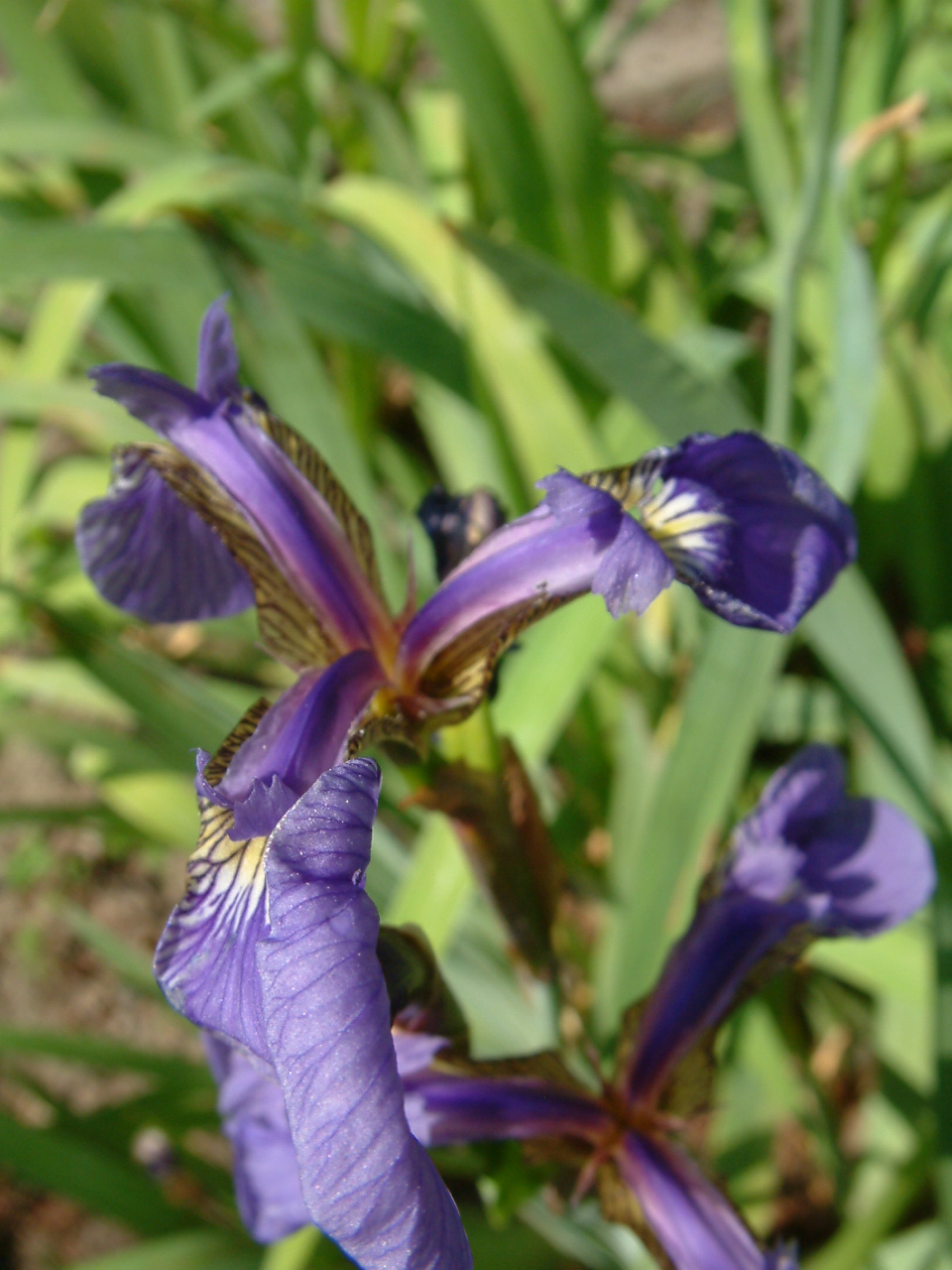 |  |  \n\nThe chart above shows three different kinds of the Iris flowers. \n\nWe will use sepal length, sepal width, petal length, petal width as the feature and species as the label to train the model.\n\n### Sklearn Model\n\nYou can find more information [here](http://onnx.ai/sklearn-onnx/). You can use the sklearn built-in iris dataset to load the data. Then we defined a [RandomForestClassifer](https://scikit-learn.org/stable/modules/generated/sklearn.ensemble.RandomForestClassifier.html) to train the model. After that, we convert the model to onnx format for DJL to run inference. The following code is a sample classification setup using sklearn:\n\n```python\n# Train a model.\nfrom sklearn.datasets import load_iris\nfrom sklearn.model_selection import train_test_split\nfrom sklearn.ensemble import RandomForestClassifier\niris = load_iris()\nX, y = iris.data, iris.target\nX_train, X_test, y_train, y_test = train_test_split(X, y)\nclr = RandomForestClassifier()\nclr.fit(X_train, y_train)\n```\n\n\n## Preparation\n\nThis tutorial requires the installation of Java Kernel. To install the Java Kernel, see the [README](https://github.com/awslabs/djl/blob/master/jupyter/README.md).\n\nThese are dependencies we will use. To enhance the NDArray operation capability, we are importing ONNX Runtime and PyTorch Engine at the same time. Please find more information [here](https://github.com/awslabs/djl/blob/master/docs/onnxruntime/hybrid_engine.md#hybrid-engine-for-onnx-runtime).",
"_____no_output_____"
]
],
[
[
"// %mavenRepo snapshots https://oss.sonatype.org/content/repositories/snapshots/\n\n%maven ai.djl:api:0.8.0\n%maven ai.djl.onnxruntime:onnxruntime-engine:0.8.0\n%maven ai.djl.pytorch:pytorch-engine:0.8.0\n%maven org.slf4j:slf4j-api:1.7.26\n%maven org.slf4j:slf4j-simple:1.7.26\n\n%maven com.microsoft.onnxruntime:onnxruntime:1.4.0\n%maven ai.djl.pytorch:pytorch-native-auto:1.6.0",
"_____no_output_____"
],
[
"import ai.djl.inference.*;\nimport ai.djl.modality.*;\nimport ai.djl.ndarray.*;\nimport ai.djl.ndarray.types.*;\nimport ai.djl.repository.zoo.*;\nimport ai.djl.translate.*;\nimport java.util.*;",
"_____no_output_____"
]
],
[
[
"## Step 1 create a Translator\n\nInference in machine learning is the process of predicting the output for a given input based on a pre-defined model.\nDJL abstracts away the whole process for ease of use. It can load the model, perform inference on the input, and provide\noutput. DJL also allows you to provide user-defined inputs. The workflow looks like the following:\n\n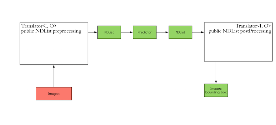\n\nThe `Translator` interface encompasses the two white blocks: Pre-processing and Post-processing. The pre-processing\ncomponent converts the user-defined input objects into an NDList, so that the `Predictor` in DJL can understand the\ninput and make its prediction. Similarly, the post-processing block receives an NDList as the output from the\n`Predictor`. The post-processing block allows you to convert the output from the `Predictor` to the desired output\nformat.\n\nIn our use case, we use a class namely `IrisFlower` as our input class type. We will use [`Classifications`](https://javadoc.io/doc/ai.djl/api/latest/ai/djl/modality/Classifications.html) as our output class type.",
"_____no_output_____"
]
],
[
[
"public static class IrisFlower {\n\n public float sepalLength;\n public float sepalWidth;\n public float petalLength;\n public float petalWidth;\n\n public IrisFlower(float sepalLength, float sepalWidth, float petalLength, float petalWidth) {\n this.sepalLength = sepalLength;\n this.sepalWidth = sepalWidth;\n this.petalLength = petalLength;\n this.petalWidth = petalWidth;\n }\n}",
"_____no_output_____"
]
],
[
[
"Let's create a translator",
"_____no_output_____"
]
],
[
[
"public static class MyTranslator implements Translator<IrisFlower, Classifications> {\n\n private final List<String> synset;\n\n public MyTranslator() {\n // species name\n synset = Arrays.asList(\"setosa\", \"versicolor\", \"virginica\");\n }\n\n @Override\n public NDList processInput(TranslatorContext ctx, IrisFlower input) {\n float[] data = {input.sepalLength, input.sepalWidth, input.petalLength, input.petalWidth};\n NDArray array = ctx.getNDManager().create(data, new Shape(1, 4));\n return new NDList(array);\n }\n\n @Override\n public Classifications processOutput(TranslatorContext ctx, NDList list) {\n return new Classifications(synset, list.get(1));\n }\n\n @Override\n public Batchifier getBatchifier() {\n return null;\n }\n}",
"_____no_output_____"
]
],
[
[
"## Step 2 Prepare your model\n\nWe will load a pretrained sklearn model into DJL. We defined a [`ModelZoo`](https://javadoc.io/doc/ai.djl/api/latest/ai/djl/repository/zoo/ModelZoo.html) concept to allow user load model from varity of locations, such as remote URL, local files or DJL pretrained model zoo. We need to define `Criteria` class to help the modelzoo locate the model and attach translator. In this example, we download a compressed ONNX model from S3.",
"_____no_output_____"
]
],
[
[
"String modelUrl = \"https://mlrepo.djl.ai/model/tabular/random_forest/ai/djl/onnxruntime/iris_flowers/0.0.1/iris_flowers.zip\";\nCriteria<IrisFlower, Classifications> criteria = Criteria.builder()\n .setTypes(IrisFlower.class, Classifications.class)\n .optModelUrls(modelUrl)\n .optTranslator(new MyTranslator())\n .optEngine(\"OnnxRuntime\") // use OnnxRuntime engine by default\n .build();\nZooModel<IrisFlower, Classifications> model = ModelZoo.loadModel(criteria);",
"_____no_output_____"
]
],
[
[
"## Step 3 Run inference\n\nUser will just need to create a `Predictor` from model to run the inference.",
"_____no_output_____"
]
],
[
[
"Predictor<IrisFlower, Classifications> predictor = model.newPredictor();\nIrisFlower info = new IrisFlower(1.0f, 2.0f, 3.0f, 4.0f);\npredictor.predict(info);",
"_____no_output_____"
]
]
] |
[
"markdown",
"code",
"markdown",
"code",
"markdown",
"code",
"markdown",
"code",
"markdown",
"code"
] |
[
[
"markdown"
],
[
"code",
"code"
],
[
"markdown"
],
[
"code"
],
[
"markdown"
],
[
"code"
],
[
"markdown"
],
[
"code"
],
[
"markdown"
],
[
"code"
]
] |
d00080cae9b7a28ebc8ef5ae33eb9e79b8f215bf
| 5,019
|
ipynb
|
Jupyter Notebook
|
Algorithms/landsat_radiance.ipynb
|
OIEIEIO/earthengine-py-notebooks
|
5d6c5cdec0c73bf02020ee17d42c9e30d633349f
|
[
"MIT"
] | 1,008
|
2020-01-27T02:03:18.000Z
|
2022-03-24T10:42:14.000Z
|
Algorithms/landsat_radiance.ipynb
|
rafatieppo/earthengine-py-notebooks
|
99fbc4abd1fb6ba41e3d8a55f8911217353a3237
|
[
"MIT"
] | 8
|
2020-02-01T20:18:18.000Z
|
2021-11-23T01:48:02.000Z
|
Algorithms/landsat_radiance.ipynb
|
rafatieppo/earthengine-py-notebooks
|
99fbc4abd1fb6ba41e3d8a55f8911217353a3237
|
[
"MIT"
] | 325
|
2020-01-27T02:03:36.000Z
|
2022-03-25T20:33:33.000Z
| 36.635036
| 470
| 0.557282
|
[
[
[
"<table class=\"ee-notebook-buttons\" align=\"left\">\n <td><a target=\"_blank\" href=\"https://github.com/giswqs/earthengine-py-notebooks/tree/master/Algorithms/landsat_radiance.ipynb\"><img width=32px src=\"https://www.tensorflow.org/images/GitHub-Mark-32px.png\" /> View source on GitHub</a></td>\n <td><a target=\"_blank\" href=\"https://nbviewer.jupyter.org/github/giswqs/earthengine-py-notebooks/blob/master/Algorithms/landsat_radiance.ipynb\"><img width=26px src=\"https://upload.wikimedia.org/wikipedia/commons/thumb/3/38/Jupyter_logo.svg/883px-Jupyter_logo.svg.png\" />Notebook Viewer</a></td>\n <td><a target=\"_blank\" href=\"https://colab.research.google.com/github/giswqs/earthengine-py-notebooks/blob/master/Algorithms/landsat_radiance.ipynb\"><img src=\"https://www.tensorflow.org/images/colab_logo_32px.png\" /> Run in Google Colab</a></td>\n</table>",
"_____no_output_____"
],
[
"## Install Earth Engine API and geemap\nInstall the [Earth Engine Python API](https://developers.google.com/earth-engine/python_install) and [geemap](https://geemap.org). The **geemap** Python package is built upon the [ipyleaflet](https://github.com/jupyter-widgets/ipyleaflet) and [folium](https://github.com/python-visualization/folium) packages and implements several methods for interacting with Earth Engine data layers, such as `Map.addLayer()`, `Map.setCenter()`, and `Map.centerObject()`.\nThe following script checks if the geemap package has been installed. If not, it will install geemap, which automatically installs its [dependencies](https://github.com/giswqs/geemap#dependencies), including earthengine-api, folium, and ipyleaflet.",
"_____no_output_____"
]
],
[
[
"# Installs geemap package\nimport subprocess\n\ntry:\n import geemap\nexcept ImportError:\n print('Installing geemap ...')\n subprocess.check_call([\"python\", '-m', 'pip', 'install', 'geemap'])",
"_____no_output_____"
],
[
"import ee\nimport geemap",
"_____no_output_____"
]
],
[
[
"## Create an interactive map \nThe default basemap is `Google Maps`. [Additional basemaps](https://github.com/giswqs/geemap/blob/master/geemap/basemaps.py) can be added using the `Map.add_basemap()` function. ",
"_____no_output_____"
]
],
[
[
"Map = geemap.Map(center=[40,-100], zoom=4)\nMap",
"_____no_output_____"
]
],
[
[
"## Add Earth Engine Python script ",
"_____no_output_____"
]
],
[
[
"# Add Earth Engine dataset\n# Load a raw Landsat scene and display it.\nraw = ee.Image('LANDSAT/LC08/C01/T1/LC08_044034_20140318')\nMap.centerObject(raw, 10)\nMap.addLayer(raw, {'bands': ['B4', 'B3', 'B2'], 'min': 6000, 'max': 12000}, 'raw')\n\n# Convert the raw data to radiance.\nradiance = ee.Algorithms.Landsat.calibratedRadiance(raw)\nMap.addLayer(radiance, {'bands': ['B4', 'B3', 'B2'], 'max': 90}, 'radiance')\n\n# Convert the raw data to top-of-atmosphere reflectance.\ntoa = ee.Algorithms.Landsat.TOA(raw)\n\nMap.addLayer(toa, {'bands': ['B4', 'B3', 'B2'], 'max': 0.2}, 'toa reflectance')\n\n",
"_____no_output_____"
]
],
[
[
"## Display Earth Engine data layers ",
"_____no_output_____"
]
],
[
[
"Map.addLayerControl() # This line is not needed for ipyleaflet-based Map.\nMap",
"_____no_output_____"
]
]
] |
[
"markdown",
"code",
"markdown",
"code",
"markdown",
"code",
"markdown",
"code"
] |
[
[
"markdown",
"markdown"
],
[
"code",
"code"
],
[
"markdown"
],
[
"code"
],
[
"markdown"
],
[
"code"
],
[
"markdown"
],
[
"code"
]
] |
d0008b5894090e9887e8ce1ff35481414c1bb8d4
| 22,698
|
ipynb
|
Jupyter Notebook
|
cp2/cp2_method0.ipynb
|
jet-code/multivariable-control-systems
|
81b57d51a4dfc92964f989794f71d525af0359ff
|
[
"MIT"
] | null | null | null |
cp2/cp2_method0.ipynb
|
jet-code/multivariable-control-systems
|
81b57d51a4dfc92964f989794f71d525af0359ff
|
[
"MIT"
] | null | null | null |
cp2/cp2_method0.ipynb
|
jet-code/multivariable-control-systems
|
81b57d51a4dfc92964f989794f71d525af0359ff
|
[
"MIT"
] | null | null | null | 22.858006
| 89
| 0.390475
|
[
[
[
"empty"
]
]
] |
[
"empty"
] |
[
[
"empty"
]
] |
d0009800054b678bfad6c1462b810393ddac51b0
| 217,601
|
ipynb
|
Jupyter Notebook
|
MNIST/Session2/3_Global_Average_Pooling.ipynb
|
gmshashank/pytorch_vision
|
54367b83e9780fe14c6f8b93157091ffdf7266eb
|
[
"MIT"
] | null | null | null |
MNIST/Session2/3_Global_Average_Pooling.ipynb
|
gmshashank/pytorch_vision
|
54367b83e9780fe14c6f8b93157091ffdf7266eb
|
[
"MIT"
] | null | null | null |
MNIST/Session2/3_Global_Average_Pooling.ipynb
|
gmshashank/pytorch_vision
|
54367b83e9780fe14c6f8b93157091ffdf7266eb
|
[
"MIT"
] | null | null | null | 101.209767
| 53,662
| 0.792552
|
[
[
[
"# Import Libraries",
"_____no_output_____"
]
],
[
[
"from __future__ import print_function\nimport torch\nimport torch.nn as nn\nimport torch.nn.functional as F\nimport torch.optim as optim\nimport torchvision\nfrom torchvision import datasets, transforms",
"_____no_output_____"
],
[
"%matplotlib inline\r\nimport matplotlib.pyplot as plt",
"_____no_output_____"
]
],
[
[
"## Data Transformations\n\nWe first start with defining our data transformations. We need to think what our data is and how can we augment it to correct represent images which it might not see otherwise. \n",
"_____no_output_____"
]
],
[
[
"# Train Phase transformations\ntrain_transforms = transforms.Compose([\n # transforms.Resize((28, 28)),\n # transforms.ColorJitter(brightness=0.10, contrast=0.1, saturation=0.10, hue=0.1),\n transforms.ToTensor(),\n transforms.Normalize((0.1307,), (0.3081,)) # The mean and std have to be sequences (e.g., tuples), therefore you should add a comma after the values. \n # Note the difference between (0.1307) and (0.1307,)\n ])\n\n# Test Phase transformations\ntest_transforms = transforms.Compose([\n # transforms.Resize((28, 28)),\n # transforms.ColorJitter(brightness=0.10, contrast=0.1, saturation=0.10, hue=0.1),\n transforms.ToTensor(),\n transforms.Normalize((0.1307,), (0.3081,))\n ])\n",
"_____no_output_____"
]
],
[
[
"# Dataset and Creating Train/Test Split",
"_____no_output_____"
]
],
[
[
"train = datasets.MNIST('./data', train=True, download=True, transform=train_transforms)\ntest = datasets.MNIST('./data', train=False, download=True, transform=test_transforms)",
"Downloading http://yann.lecun.com/exdb/mnist/train-images-idx3-ubyte.gz to ./data/MNIST/raw/train-images-idx3-ubyte.gz\n"
]
],
[
[
"# Dataloader Arguments & Test/Train Dataloaders\n",
"_____no_output_____"
]
],
[
[
"SEED = 1\n\n# CUDA?\ncuda = torch.cuda.is_available()\nprint(\"CUDA Available?\", cuda)\n\n# For reproducibility\ntorch.manual_seed(SEED)\n\nif cuda:\n torch.cuda.manual_seed(SEED)\n\n# dataloader arguments - something you'll fetch these from cmdprmt\ndataloader_args = dict(shuffle=True, batch_size=128, num_workers=4, pin_memory=True) if cuda else dict(shuffle=True, batch_size=64)\n\n# train dataloader\ntrain_loader = torch.utils.data.DataLoader(train, **dataloader_args)\n\n# test dataloader\ntest_loader = torch.utils.data.DataLoader(test, **dataloader_args)",
"CUDA Available? True\n"
]
],
[
[
"# Data Statistics\n\nIt is important to know your data very well. Let's check some of the statistics around our data and how it actually looks like",
"_____no_output_____"
]
],
[
[
"# We'd need to convert it into Numpy! Remember above we have converted it into tensors already\ntrain_data = train.train_data\ntrain_data = train.transform(train_data.numpy())\n\nprint('[Train]')\nprint(' - Numpy Shape:', train.train_data.cpu().numpy().shape)\nprint(' - Tensor Shape:', train.train_data.size())\nprint(' - min:', torch.min(train_data))\nprint(' - max:', torch.max(train_data))\nprint(' - mean:', torch.mean(train_data))\nprint(' - std:', torch.std(train_data))\nprint(' - var:', torch.var(train_data))\n\ndataiter = iter(train_loader)\nimages, labels = dataiter.next()\n\nprint(images.shape)\nprint(labels.shape)\n\n# Let's visualize some of the images\nplt.imshow(images[0].numpy().squeeze(), cmap='gray_r')",
"\n"
]
],
[
[
"## MORE\n\nIt is important that we view as many images as possible. This is required to get some idea on image augmentation later on",
"_____no_output_____"
]
],
[
[
"figure = plt.figure()\nnum_of_images = 60\nfor index in range(1, num_of_images + 1):\n plt.subplot(6, 10, index)\n plt.axis('off')\n plt.imshow(images[index].numpy().squeeze(), cmap='gray_r')",
"_____no_output_____"
]
],
[
[
"# The model\nLet's start with the model we first saw",
"_____no_output_____"
]
],
[
[
"class Net(nn.Module):\n def __init__(self):\n super(Net, self).__init__()\n # Input Block\n self.convblock1 = nn.Sequential(\n nn.Conv2d(in_channels=1, out_channels=16, kernel_size=(3, 3), padding=0, bias=False),\n nn.ReLU(),\n ) # output_size = 26\n\n # CONVOLUTION BLOCK 1\n self.convblock2 = nn.Sequential(\n nn.Conv2d(in_channels=16, out_channels=16, kernel_size=(3, 3), padding=0, bias=False),\n nn.ReLU(),\n ) # output_size = 24\n\n # TRANSITION BLOCK 1\n self.convblock3 = nn.Sequential(\n nn.Conv2d(in_channels=16, out_channels=16, kernel_size=(1, 1), padding=0, bias=False),\n nn.ReLU(),\n ) # output_size = 24\n self.pool1 = nn.MaxPool2d(2, 2) # output_size = 12\n\n # CONVOLUTION BLOCK 2\n self.convblock4 = nn.Sequential(\n nn.Conv2d(in_channels=16, out_channels=16, kernel_size=(3, 3), padding=0, bias=False),\n nn.ReLU(),\n ) # output_size = 10\n\n self.convblock5 = nn.Sequential(\n nn.Conv2d(in_channels=16, out_channels=16, kernel_size=(3, 3), padding=0, bias=False),\n nn.ReLU(),\n ) # output_size = 8\n self.convblock6 = nn.Sequential(\n nn.Conv2d(in_channels=16, out_channels=10, kernel_size=(3, 3), padding=0, bias=False),\n nn.ReLU(),\n ) # output_size = 6\n\n # OUTPUT BLOCK\n self.convblock7 = nn.Sequential(\n nn.Conv2d(in_channels=10, out_channels=10, kernel_size=(3, 3), padding=1, bias=False),\n nn.ReLU(),\n ) # output_size = 6\n\n self.gap = nn.Sequential(\n nn.AvgPool2d(kernel_size=6)\n )\n\n self.convblock8 = nn.Sequential(\n nn.Conv2d(in_channels=10, out_channels=10, kernel_size=(1, 1), padding=0, bias=False),\n # nn.BatchNorm2d(10), NEVER\n # nn.ReLU() NEVER!\n ) # output_size = 1\n\n def forward(self, x):\n x = self.convblock1(x)\n x = self.convblock2(x)\n x = self.convblock3(x)\n x = self.pool1(x)\n x = self.convblock4(x)\n x = self.convblock5(x)\n x = self.convblock6(x)\n x = self.convblock7(x)\n x = self.gap(x)\n x = self.convblock8(x)\n x = x.view(-1, 10)\n return F.log_softmax(x, dim=-1)",
"_____no_output_____"
]
],
[
[
"# Model Params\nCan't emphasize on how important viewing Model Summary is. \nUnfortunately, there is no in-built model visualizer, so we have to take external help",
"_____no_output_____"
]
],
[
[
"!pip install torchsummary\nfrom torchsummary import summary\nuse_cuda = torch.cuda.is_available()\ndevice = torch.device(\"cuda\" if use_cuda else \"cpu\")\nprint(device)\nmodel = Net().to(device)\nsummary(model, input_size=(1, 28, 28))\n",
"Requirement already satisfied: torchsummary in /usr/local/lib/python3.6/dist-packages (1.5.1)\ncuda\n----------------------------------------------------------------\n Layer (type) Output Shape Param #\n================================================================\n Conv2d-1 [-1, 16, 26, 26] 144\n ReLU-2 [-1, 16, 26, 26] 0\n Conv2d-3 [-1, 16, 24, 24] 2,304\n ReLU-4 [-1, 16, 24, 24] 0\n Conv2d-5 [-1, 16, 24, 24] 256\n ReLU-6 [-1, 16, 24, 24] 0\n MaxPool2d-7 [-1, 16, 12, 12] 0\n Conv2d-8 [-1, 16, 10, 10] 2,304\n ReLU-9 [-1, 16, 10, 10] 0\n Conv2d-10 [-1, 16, 8, 8] 2,304\n ReLU-11 [-1, 16, 8, 8] 0\n Conv2d-12 [-1, 10, 6, 6] 1,440\n ReLU-13 [-1, 10, 6, 6] 0\n Conv2d-14 [-1, 10, 6, 6] 900\n ReLU-15 [-1, 10, 6, 6] 0\n AvgPool2d-16 [-1, 10, 1, 1] 0\n Conv2d-17 [-1, 10, 1, 1] 100\n================================================================\nTotal params: 9,752\nTrainable params: 9,752\nNon-trainable params: 0\n----------------------------------------------------------------\nInput size (MB): 0.00\nForward/backward pass size (MB): 0.52\nParams size (MB): 0.04\nEstimated Total Size (MB): 0.56\n----------------------------------------------------------------\n"
]
],
[
[
"# Training and Testing\n\nLooking at logs can be boring, so we'll introduce **tqdm** progressbar to get cooler logs. \n\nLet's write train and test functions",
"_____no_output_____"
]
],
[
[
"from tqdm import tqdm\n\ntrain_losses = []\ntest_losses = []\ntrain_acc = []\ntest_acc = []\n\ndef train(model, device, train_loader, optimizer, epoch):\n\n global train_max\n model.train()\n pbar = tqdm(train_loader)\n correct = 0\n processed = 0\n for batch_idx, (data, target) in enumerate(pbar):\n # get samples\n data, target = data.to(device), target.to(device)\n\n # Init\n optimizer.zero_grad()\n # In PyTorch, we need to set the gradients to zero before starting to do backpropragation because PyTorch accumulates the gradients on subsequent backward passes. \n # Because of this, when you start your training loop, ideally you should zero out the gradients so that you do the parameter update correctly.\n\n # Predict\n y_pred = model(data)\n\n # Calculate loss\n loss = F.nll_loss(y_pred, target)\n train_losses.append(loss)\n \n # Backpropagation\n loss.backward()\n optimizer.step()\n\n # Update pbar-tqdm\n \n pred = y_pred.argmax(dim=1, keepdim=True) # get the index of the max log-probability\n correct += pred.eq(target.view_as(pred)).sum().item()\n processed += len(data)\n \n pbar.set_description(desc= f'Loss={loss.item()} Batch_id={batch_idx} Accuracy={100*correct/processed:0.2f}')\n train_acc.append(100*correct/processed)\n \n if (train_max < 100*correct/processed):\n train_max = 100*correct/processed\n\n\ndef test(model, device, test_loader):\n\n global test_max\n model.eval()\n test_loss = 0\n correct = 0\n with torch.no_grad():\n for data, target in test_loader:\n data, target = data.to(device), target.to(device)\n output = model(data)\n test_loss += F.nll_loss(output, target, reduction='sum').item() # sum up batch loss\n pred = output.argmax(dim=1, keepdim=True) # get the index of the max log-probability\n correct += pred.eq(target.view_as(pred)).sum().item()\n\n test_loss /= len(test_loader.dataset)\n test_losses.append(test_loss)\n\n print('\\nTest set: Average loss: {:.4f}, Accuracy: {}/{} ({:.2f}%)\\n'.format(\n test_loss, correct, len(test_loader.dataset),\n 100. * correct / len(test_loader.dataset)))\n\n if (test_max < 100. * correct / len(test_loader.dataset)):\n test_max = 100. * correct / len(test_loader.dataset)\n \n test_acc.append(100. * correct / len(test_loader.dataset))\n",
"_____no_output_____"
]
],
[
[
"# Let's Train and test our model",
"_____no_output_____"
]
],
[
[
"model = Net().to(device)\noptimizer = optim.SGD(model.parameters(), lr=0.01, momentum=0.9)\nEPOCHS = 15\ntrain_max=0\ntest_max=0\nfor epoch in range(EPOCHS):\n print(\"EPOCH:\", epoch)\n train(model, device, train_loader, optimizer, epoch)\n test(model, device, test_loader)\n\nprint(f\"\\nMaximum training accuracy: {train_max}\\n\")\nprint(f\"\\nMaximum test accuracy: {test_max}\\n\")\n",
"\r 0%| | 0/469 [00:00<?, ?it/s]"
],
[
"fig, axs = plt.subplots(2,2,figsize=(15,10))\naxs[0, 0].plot(train_losses)\naxs[0, 0].set_title(\"Training Loss\")\naxs[1, 0].plot(train_acc)\naxs[1, 0].set_title(\"Training Accuracy\")\naxs[0, 1].plot(test_losses)\naxs[0, 1].set_title(\"Test Loss\")\naxs[1, 1].plot(test_acc)\naxs[1, 1].set_title(\"Test Accuracy\")",
"_____no_output_____"
],
[
"fig, ((axs1, axs2), (axs3, axs4)) = plt.subplots(2,2,figsize=(15,10)) \r\n# Train plot\r\naxs1.plot(train_losses)\r\naxs1.set_title(\"Training Loss\")\r\naxs3.plot(train_acc)\r\naxs3.set_title(\"Training Accuracy\")\r\n\r\n# axs1.set_xlim([0, 5])\r\naxs1.set_ylim([0, 5])\r\naxs3.set_ylim([0, 100])\r\n\r\n\r\n# Test plot\r\naxs2.plot(test_losses)\r\naxs2.set_title(\"Test Loss\")\r\naxs4.plot(test_acc)\r\naxs4.set_title(\"Test Accuracy\")\r\n\r\naxs2.set_ylim([0, 5])\r\naxs4.set_ylim([0, 100])\r\n",
"_____no_output_____"
],
[
"",
"_____no_output_____"
]
]
] |
[
"markdown",
"code",
"markdown",
"code",
"markdown",
"code",
"markdown",
"code",
"markdown",
"code",
"markdown",
"code",
"markdown",
"code",
"markdown",
"code",
"markdown",
"code",
"markdown",
"code"
] |
[
[
"markdown"
],
[
"code",
"code"
],
[
"markdown"
],
[
"code"
],
[
"markdown"
],
[
"code"
],
[
"markdown"
],
[
"code"
],
[
"markdown"
],
[
"code"
],
[
"markdown"
],
[
"code"
],
[
"markdown"
],
[
"code"
],
[
"markdown"
],
[
"code"
],
[
"markdown"
],
[
"code"
],
[
"markdown"
],
[
"code",
"code",
"code",
"code"
]
] |
End of preview. Expand
in Data Studio
- Downloads last month
- 1,659