Deep Dive: Vision Transformers On Hugging Face Optimum Graphcore

This blog post will show how easy it is to fine-tune pre-trained Transformer models for your dataset using the Hugging Face Optimum library on Graphcore Intelligence Processing Units (IPUs). As an example, we will show a step-by-step guide and provide a notebook that takes a large, widely-used chest X-ray dataset and trains a vision transformer (ViT) model.
Introducing vision transformer (ViT) models
In 2017 a group of Google AI researchers published a paper introducing the transformer model architecture. Characterised by a novel self-attention mechanism, transformers were proposed as a new and efficient group of models for language applications. Indeed, in the last five years, transformers have seen explosive popularity and are now accepted as the de facto standard for natural language processing (NLP).
Transformers for language are perhaps most notably represented by the rapidly evolving GPT and BERT model families. Both can run easily and efficiently on Graphcore IPUs as part of the growing Hugging Face Optimum Graphcore library).
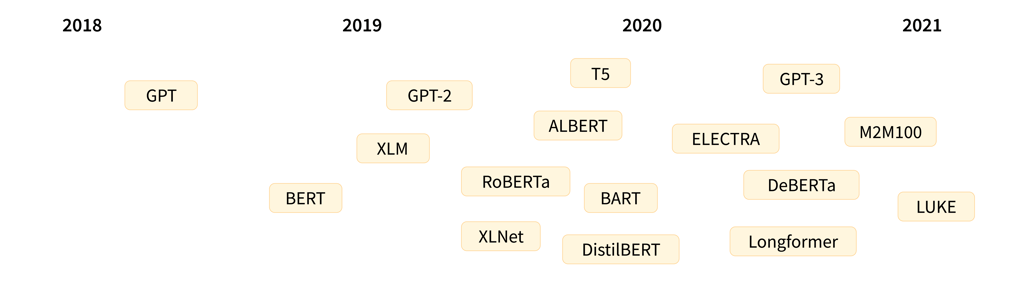
A timeline showing releases of prominent transformer language models (credit: Hugging Face)
An in-depth explainer about the transformer model architecture (with a focus on NLP) can be found on the Hugging Face website.
While transformers have seen initial success in language, they are extremely versatile and can be used for a range of other purposes including computer vision (CV), as we will cover in this blog post.
CV is an area where convolutional neural networks (CNNs) are without doubt the most popular architecture. However, the vision transformer (ViT) architecture, first introduced in a 2021 paper from Google Research, represents a breakthrough in image recognition and uses the same self-attention mechanism as BERT and GPT as its main component.
Whereas BERT and other transformer-based language processing models take a sentence (i.e., a list of words) as input, ViT models divide an input image into several small patches, equivalent to individual words in language processing. Each patch is linearly encoded by the transformer model into a vector representation that can be processed individually. This approach of splitting images into patches, or visual tokens, stands in contrast to the pixel arrays used by CNNs.
Thanks to pre-training, the ViT model learns an inner representation of images that can then be used to extract visual features useful for downstream tasks. For instance, you can train a classifier on a new dataset of labelled images by placing a linear layer on top of the pre-trained visual encoder. One typically places a linear layer on top of the [CLS] token, as the last hidden state of this token can be seen as a representation of an entire image.
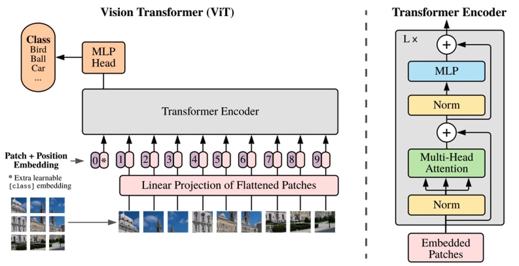
An overview of the ViT model structure as introduced in Google Research’s original 2021 paper
Compared to CNNs, ViT models have displayed higher recognition accuracy with lower computational cost, and are applied to a range of applications including image classification, object detection, and segmentation. Use cases in the healthcare domain alone include detection and classification for COVID-19, femur fractures, emphysema, breast cancer, and Alzheimer’s disease—among many others.
ViT models – a perfect fit for IPU
Graphcore IPUs are particularly well-suited to ViT models due to their ability to parallelise training using a combination of data pipelining and model parallelism. Accelerating this massively parallel process is made possible through IPU’s MIMD architecture and its scale-out solution centred on the IPU-Fabric.
By introducing pipeline parallelism, the batch size that can be processed per instance of data parallelism is increased, the access efficiency of the memory area handled by one IPU is improved, and the communication time of parameter aggregation for data parallel learning is reduced.
Thanks to the addition of a range of pre-optimized transformer models to the open-source Hugging Face Optimum Graphcore library, it’s incredibly easy to achieve a high degree of performance and efficiency when running and fine-tuning models such as ViT on IPUs.
Through Hugging Face Optimum, Graphcore has released ready-to-use IPU-trained model checkpoints and configuration files to make it easy to train models with maximum efficiency. This is particularly helpful since ViT models generally require pre-training on a large amount of data. This integration lets you use the checkpoints released by the original authors themselves within the Hugging Face model hub, so you won’t have to train them yourself. By letting users plug and play any public dataset, Optimum shortens the overall development lifecycle of AI models and allows seamless integration to Graphcore’s state-of-the-art hardware, giving a quicker time-to-value.
For this blog post, we will use a ViT model pre-trained on ImageNet-21k, based on the paper An Image is Worth 16x16 Words: Transformers for Image Recognition at Scale by Dosovitskiy et al. As an example, we will show you the process of using Optimum to fine-tune ViT on the ChestX-ray14 Dataset.
The value of ViT models for X-ray classification
As with all medical imaging tasks, radiologists spend many years learning reliably and efficiently detect problems and make tentative diagnoses on the basis of X-ray images. To a large degree, this difficulty arises from the very minute differences and spatial limitations of the images, which is why computer aided detection and diagnosis (CAD) techniques have shown such great potential for impact in improving clinician workflows and patient outcomes.
At the same time, developing any model for X-ray classification (ViT or otherwise) will entail its fair share of challenges:
- Training a model from scratch takes an enormous amount of labeled data;
- The high resolution and volume requirements mean powerful compute is necessary to train such models; and
- The complexity of multi-class and multi-label problems such as pulmonary diagnosis is exponentially compounded due to the number of disease categories.
As mentioned above, for the purpose of our demonstration using Hugging Face Optimum, we don’t need to train ViT from scratch. Instead, we will use model weights hosted in the Hugging Face model hub.
As an X-ray image can have multiple diseases, we will work with a multi-label classification model. The model in question uses google/vit-base-patch16-224-in21k checkpoints. It has been converted from the TIMM repository and pre-trained on 14 million images from ImageNet-21k. In order to parallelise and optimise the job for IPU, the configuration has been made available through the Graphcore-ViT model card.
If this is your first time using IPUs, read the IPU Programmer's Guide to learn the basic concepts. To run your own PyTorch model on the IPU see the Pytorch basics tutorial, and learn how to use Optimum through our Hugging Face Optimum Notebooks.
Training ViT on the ChestXRay-14 dataset
First, we need to download the National Institutes of Health (NIH) Clinical Center’s Chest X-ray dataset. This dataset contains 112,120 deidentified frontal view X-rays from 30,805 patients over a period from 1992 to 2015. The dataset covers a range of 14 common diseases based on labels mined from the text of radiology reports using NLP techniques.
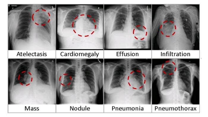
Eight visual examples of common thorax diseases (Credit: NIC)
Setting up the environment
Here are the requirements to run this walkthrough:
- A Jupyter Notebook server with the latest Poplar SDK and PopTorch environment enabled (see our guide on using IPUs from Jupyter notebooks)
- The ViT Training Notebook from the Graphcore Tutorials repo
The Graphcore Tutorials repository contains the step-by-step tutorial notebook and Python script discussed in this guide. Clone the repository and launch the walkthrough.ipynb notebook found in tutorials/tutorials/pytorch/vit_model_training/.
We’ve even made it easier and created the HF Optimum Gradient so you can launch the getting started tutorial in Free IPUs. Sign up and launch the runtime:![]()
Getting the dataset
Download the dataset's /images directory. You can use bash to extract the files: for f in images*.tar.gz; do tar xfz "$f"; done.
Next, download the Data_Entry_2017_v2020.csv file, which contains the labels. By default, the tutorial expects the /images folder and .csv file to be in the same folder as the script being run.
Once your Jupyter environment has the datasets, you need to install and import the latest Hugging Face Optimum Graphcore package and other dependencies in requirements.txt:
%pip install -r requirements.txt
The examinations contained in the Chest X-ray dataset consist of X-ray images (greyscale, 224x224 pixels) with corresponding metadata: Finding Labels, Follow-up #,Patient ID, Patient Age, Patient Gender, View Position, OriginalImage[Width Height] and OriginalImagePixelSpacing[x y].
Next, we define the locations of the downloaded images and the file with the labels to be downloaded in Getting the dataset:
We are going to train the Graphcore Optimum ViT model to predict diseases (defined by "Finding Label") from the images. "Finding Label" can be any number of 14 diseases or a "No Finding" label, which indicates that no disease was detected. To be compatible with the Hugging Face library, the text labels need to be transformed to N-hot encoded arrays representing the multiple labels which are needed to classify each image. An N-hot encoded array represents the labels as a list of booleans, true if the label corresponds to the image and false if not.
First we identify the unique labels in the dataset.
Now we transform the labels into N-hot encoded arrays:
When loading data using the datasets.load_dataset function, labels can be provided either by having folders for each of the labels (see "ImageFolder" documentation) or by having a metadata.jsonl file (see "ImageFolder with metadata" documentation). As the images in this dataset can have multiple labels, we have chosen to use a metadata.jsonl file. We write the image file names and their associated labels to the metadata.jsonl file.
Creating the dataset
We are now ready to create the PyTorch dataset and split it into training and validation sets. This step converts the dataset to the Arrow file format which allows data to be loaded quickly during training and validation (about Arrow and Hugging Face). Because the entire dataset is being loaded and pre-processed it can take a few minutes.
We are going to import the ViT model from the checkpoint google/vit-base-patch16-224-in21k. The checkpoint is a standard model hosted by Hugging Face and is not managed by Graphcore.
To fine-tune a pre-trained model, the new dataset must have the same properties as the original dataset used for pre-training. In Hugging Face, the original dataset information is provided in a config file loaded using the AutoImageProcessor. For this model, the X-ray images are resized to the correct resolution (224x224), converted from grayscale to RGB, and normalized across the RGB channels with a mean (0.5, 0.5, 0.5) and a standard deviation (0.5, 0.5, 0.5).
For the model to run efficiently, images need to be batched. To do this, we define the vit_data_collator function that returns batches of images and labels in a dictionary, following the default_data_collator pattern in Transformers Data Collator.
Visualising the dataset
To examine the dataset, we display the first 10 rows of metadata.
Let's also plot some images from the validation set with their associated labels.
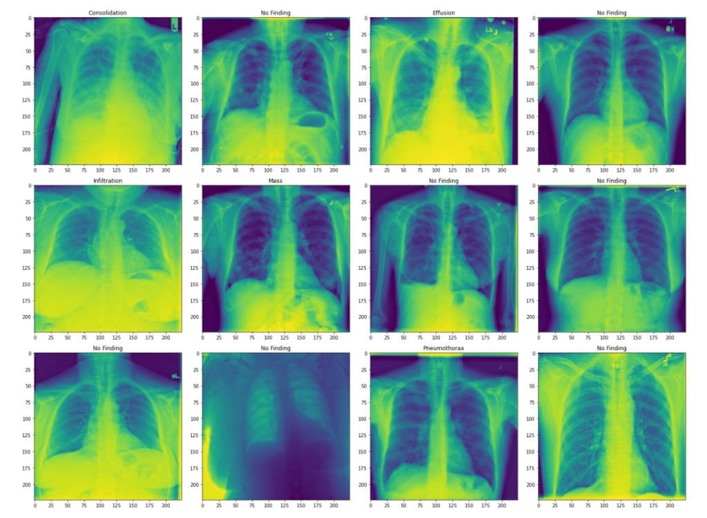
The images are chest X-rays with labels of lung diseases the patient was diagnosed with. Here, we show the transformed images.
Our dataset is now ready to be used.
Preparing the model
To train a model on the IPU we need to import it from Hugging Face Hub and define a trainer using the IPUTrainer class. The IPUTrainer class takes the same arguments as the original Transformer Trainer and works in tandem with the IPUConfig object which specifies the behaviour for compilation and execution on the IPU.
Now we import the ViT model from Hugging Face.
To use this model on the IPU we need to load the IPU configuration, IPUConfig, which gives control to all the parameters specific to Graphcore IPUs (existing IPU configs can be found here). We are going to use Graphcore/vit-base-ipu.
Let's set our training hyperparameters using IPUTrainingArguments. This subclasses the Hugging Face TrainingArguments class, adding parameters specific to the IPU and its execution characteristics.
Implementing a custom performance metric for evaluation
The performance of multi-label classification models can be assessed using the area under the ROC (receiver operating characteristic) curve (AUC_ROC). The AUC_ROC is a plot of the true positive rate (TPR) against the false positive rate (FPR) of different classes and at different threshold values. This is a commonly used performance metric for multi-label classification tasks because it is insensitive to class imbalance and easy to interpret.
For this dataset, the AUC_ROC represents the ability of the model to separate the different diseases. A score of 0.5 means that it is 50% likely to get the correct disease and a score of 1 means that it can perfectly separate the diseases. This metric is not available in Datasets, hence we need to implement it ourselves. HuggingFace Datasets package allows custom metric calculation through the load_metric() function. We define a compute_metrics function and expose it to Transformer’s evaluation function just like the other supported metrics through the datasets package. The compute_metrics function takes the labels predicted by the ViT model and computes the area under the ROC curve. The compute_metrics function takes an EvalPrediction object (a named tuple with a predictions and label_ids field), and has to return a dictionary string to float.
To train the model, we define a trainer using the IPUTrainer class which takes care of compiling the model to run on IPUs, and of performing training and evaluation. The IPUTrainer class works just like the Hugging Face Trainer class, but takes the additional ipu_config argument.
Running the training
To accelerate training we will load the last checkpoint if it exists.
Now we are ready to train.
Plotting convergence
Now that we have completed the training, we can format and plot the trainer output to evaluate the training behaviour.
We plot the training loss and the learning rate.
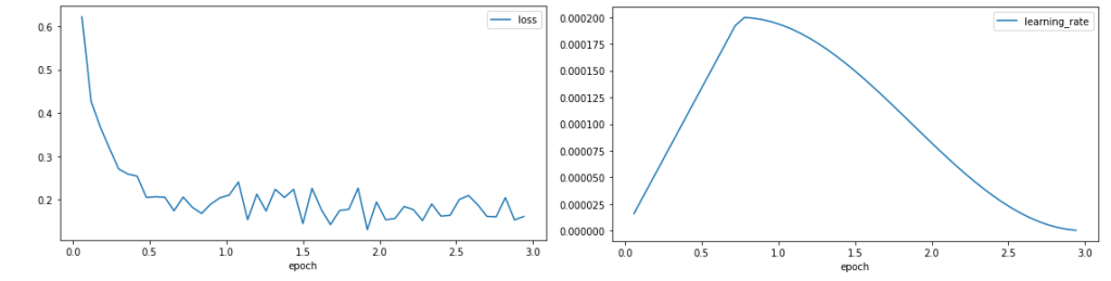 The loss curve shows a rapid reduction in the loss at the start of training before stabilising around 0.1, showing that the model is learning. The learning rate increases through the warm-up of 25% of the training period, before following a cosine decay.
Running the evaluation
Now that we have trained the model, we can evaluate its ability to predict the labels of unseen data using the validation dataset.
The metrics show the validation AUC_ROC score the tutorial achieves after 3 epochs.
There are several directions to explore to improve the accuracy of the model including longer training. The validation performance might also be improved through changing optimisers, learning rate, learning rate schedule, loss scaling, or using auto-loss scaling.
Try Hugging Face Optimum on IPUs for free
In this post, we have introduced ViT models and have provided a tutorial for training a Hugging Face Optimum model on the IPU using a local dataset.
The entire process outlined above can now be run end-to-end within minutes for free, thanks to Graphcore’s new partnership with Paperspace. Launching today, the service will provide access to a selection of Hugging Face Optimum models powered by Graphcore IPUs within Gradient—Paperspace’s web-based Jupyter notebooks.
![]()
If you’re interested in trying Hugging Face Optimum with IPUs on Paperspace Gradient including ViT, BERT, RoBERTa and more, you can sign up here and find a getting started guide here.
More Resources for Hugging Face Optimum on IPUs
- ViT Optimum tutorial code on Graphcore GitHub
- Graphcore Hugging Face Models & Datasets
- Optimum Graphcore on GitHub
This deep dive would not have been possible without extensive support, guidance, and insights from Eva Woodbridge, James Briggs, Jinchen Ge, Alexandre Payot, Thorin Farnsworth, and all others contributing from Graphcore, as well as Jeff Boudier, Julien Simon, and Michael Benayoun from Hugging Face.

