Diving deeper into policy-gradient methods

Getting the big picture

We just learned that policy-gradient methods aim to find parameters $\theta$ that maximize the expected return.

The idea is that we have a parameterized stochastic policy. In our case, a neural network outputs a probability distribution over actions. The probability of taking each action is also called the action preference.

If we take the example of CartPole-v1:

• As input, we have a state.
• As output, we have a probability distribution over actions at that state.

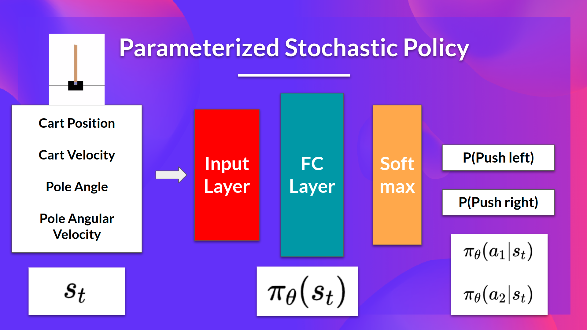
Our goal with policy-gradient is to control the probability distribution of actions by tuning the policy such that good actions (that maximize the return) are sampled more frequently in the future. Each time the agent interacts with the environment, we tweak the parameters such that good actions will be sampled more likely in the future.

But how are we going to optimize the weights using the expected return?

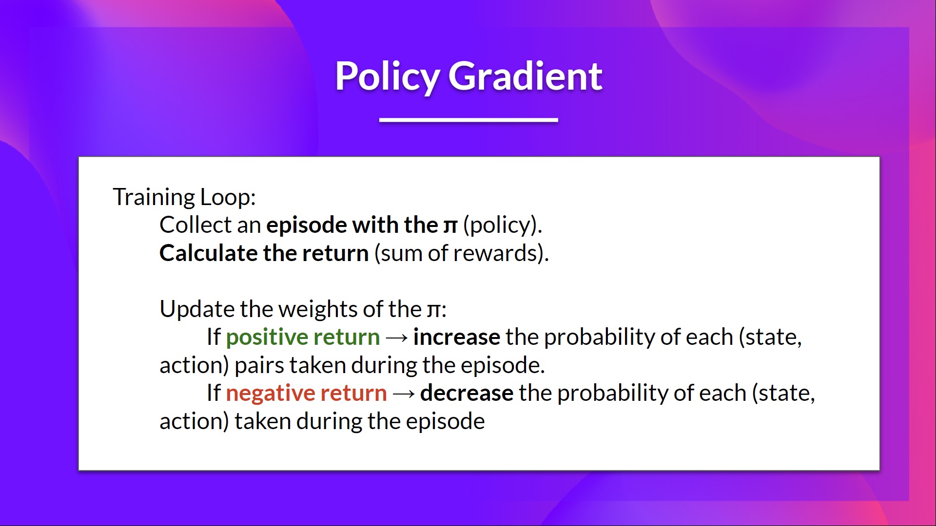
The idea is that we’re going to let the agent interact during an episode. And if we win the episode, we consider that each action taken was good and must be more sampled in the future since they lead to win.

So for each state-action pair, we want to increase the $P(a|s)$: the probability of taking that action at that state. Or decrease if we lost.

The Policy-gradient algorithm (simplified) looks like this:

Now that we got the big picture, let’s dive deeper into policy-gradient methods.

Diving deeper into policy-gradient methods

We have our stochastic policy $\pi$ which has a parameter $\theta$. This $\pi$, given a state, outputs a probability distribution of actions.

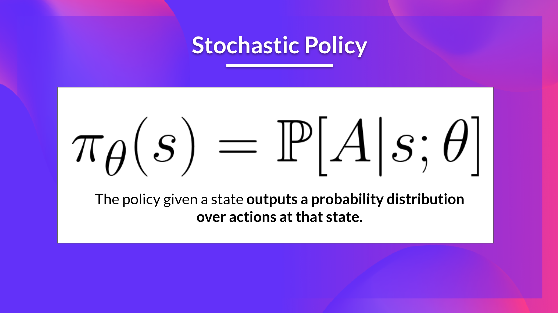
Where $\pi_\theta(a_t|s_t)$ is the probability of the agent selecting action $a_t$ from state $s_t$ given our policy.

But how do we know if our policy is good? We need to have a way to measure it. To know that, we define a score/objective function called $J(\theta)$.

The objective function

The objective function gives us the performance of the agent given a trajectory (state action sequence without considering reward (contrary to an episode)), and it outputs the expected cumulative reward.

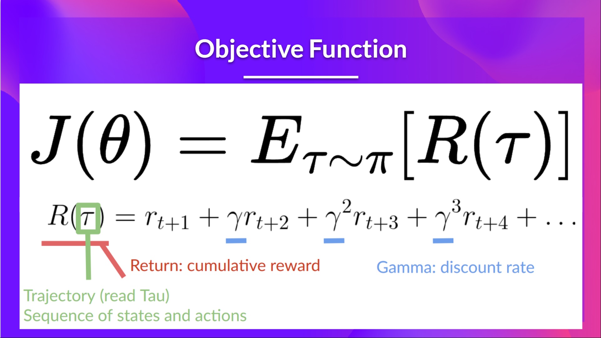
Let’s give some more details on this formula:

• The expected return (also called expected cumulative reward), is the weighted average (where the weights are given by $P(\tau;\theta)$ of all possible values that the return $R(\tau)$ can take).

-$R(\tau)$ : Return from an arbitrary trajectory. To take this quantity and use it to calculate the expected return, we need to multiply it by the probability of each possible trajectory.

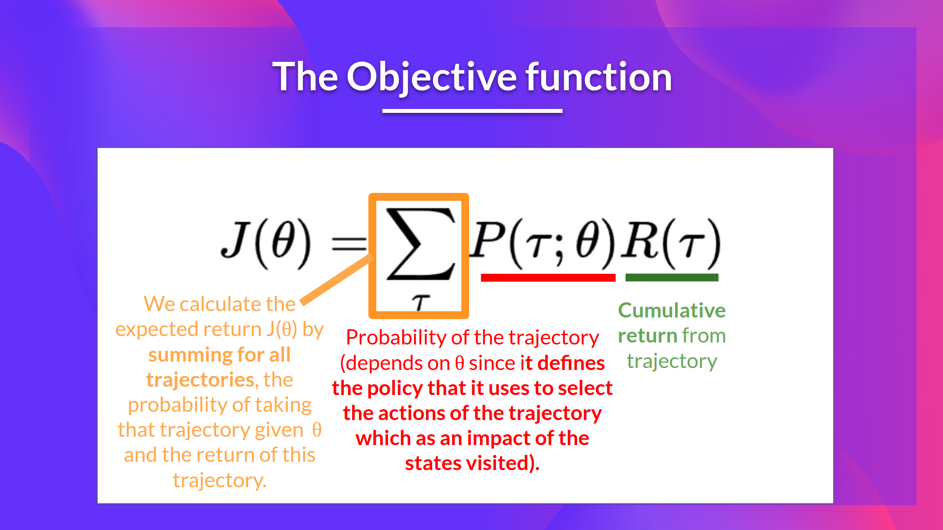
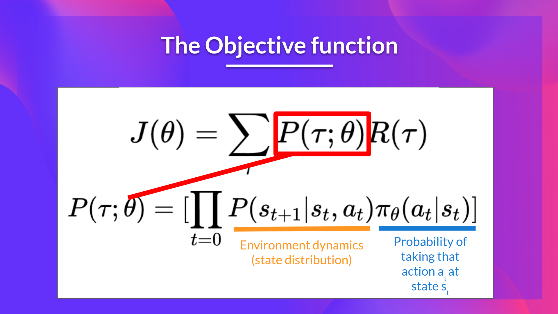
-$P(\tau;\theta)$ : Probability of each possible trajectory $\tau$ (that probability depends on $\theta$ since it defines the policy that it uses to select the actions of the trajectory which has an impact of the states visited).

-$J(\theta)$ : Expected return, we calculate it by summing for all trajectories, the probability of taking that trajectory given $\theta$ multiplied by the return of this trajectory.

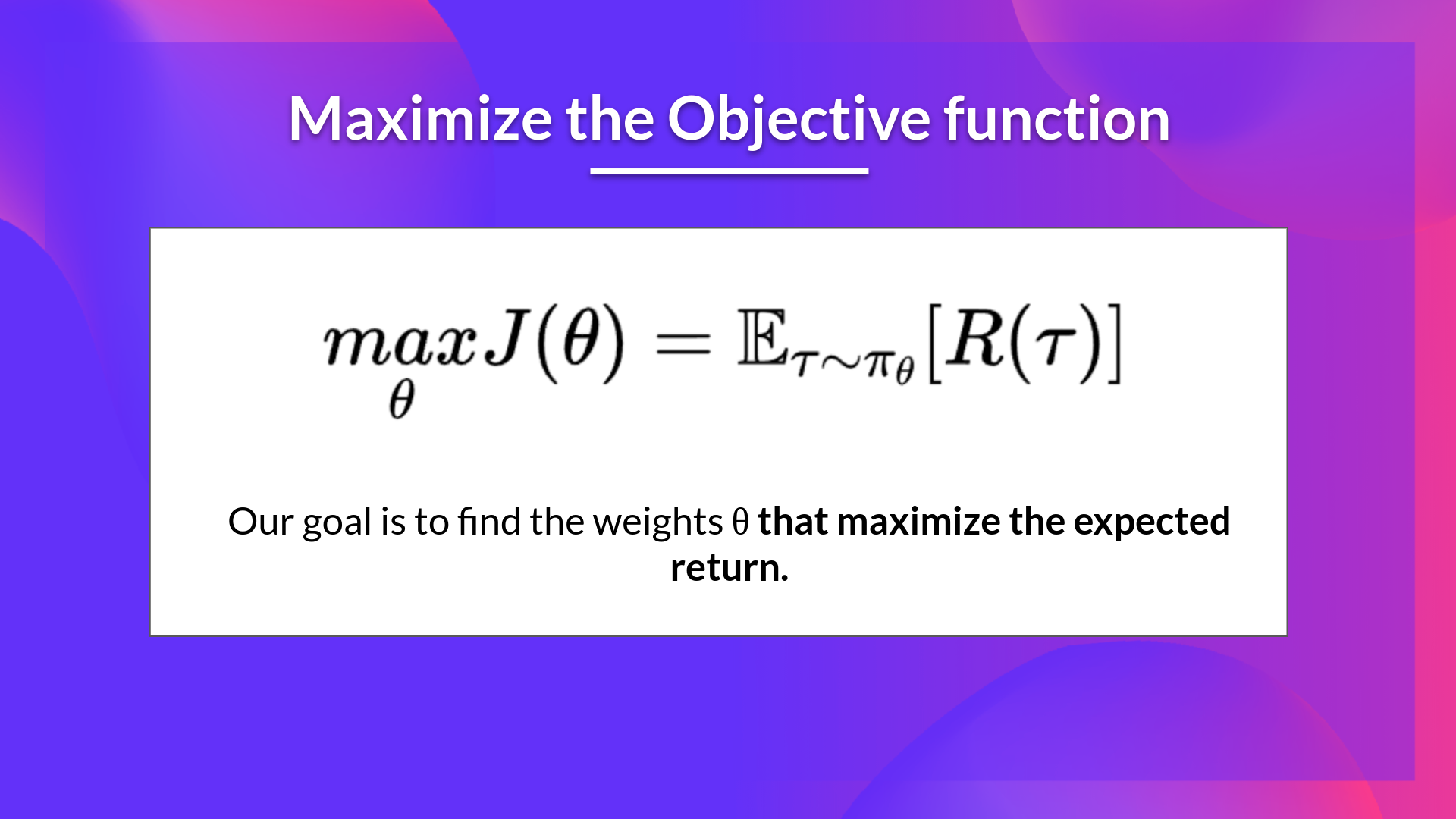
Our objective then is to maximize the expected cumulative reward by finding the $\theta$ that will output the best action probability distributions:

Gradient Ascent and the Policy-gradient Theorem

Policy-gradient is an optimization problem: we want to find the values of $\theta$ that maximize our objective function $J(\theta)$, so we need to use gradient-ascent. It’s the inverse of gradient-descent since it gives the direction of the steepest increase of $J(\theta)$.

(If you need a refresher on the difference between gradient descent and gradient ascent check this and this).

Our update step for gradient-ascent is: $\theta \leftarrow \theta + \alpha * \nabla_\theta J(\theta)$

We can repeatedly apply this update in the hopes that $\theta$ converges to the value that maximizes $J(\theta)$.

However, there are two problems with computing the derivative of $J(\theta)$:

1. We can’t calculate the true gradient of the objective function since it requires calculating the probability of each possible trajectory, which is computationally super expensive. So we want to calculate a gradient estimation with a sample-based estimate (collect some trajectories).

2. We have another problem that I explain in the next optional section. To differentiate this objective function, we need to differentiate the state distribution, called the Markov Decision Process dynamics. This is attached to the environment. It gives us the probability of the environment going into the next state, given the current state and the action taken by the agent. The problem is that we can’t differentiate it because we might not know about it.

Fortunately we’re going to use a solution called the Policy Gradient Theorem that will help us to reformulate the objective function into a differentiable function that does not involve the differentiation of the state distribution.

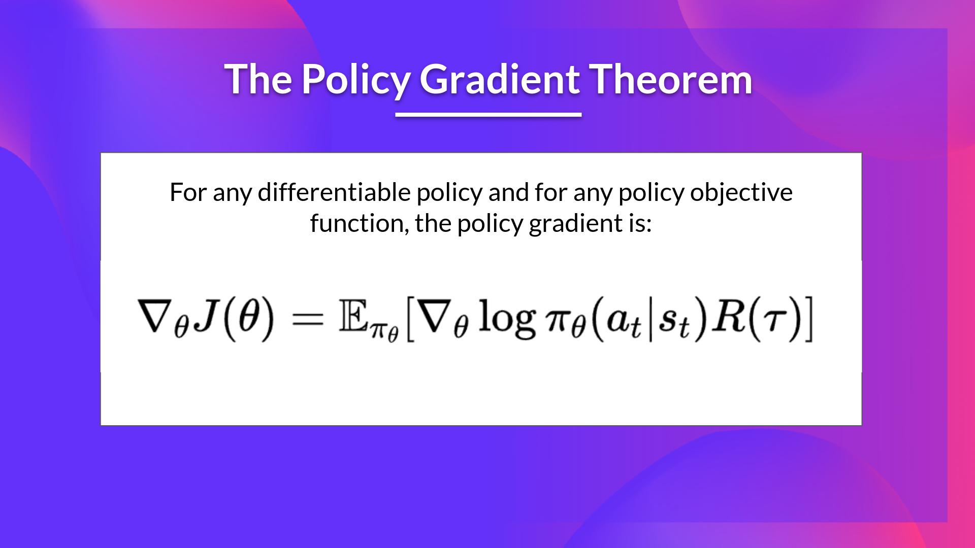
If you want to understand how we derive this formula for approximating the gradient, check out the next (optional) section.

The Reinforce algorithm (Monte Carlo Reinforce)

The Reinforce algorithm, also called Monte-Carlo policy-gradient, is a policy-gradient algorithm that uses an estimated return from an entire episode to update the policy parameter $\theta$:

In a loop:

• Use the policy $\pi_\theta$ to collect an episode $\tau$

• Use the episode to estimate the gradient $\hat{g} = \nabla_\theta J(\theta)$

  

• Update the weights of the policy: $\theta \leftarrow \theta + \alpha \hat{g}$

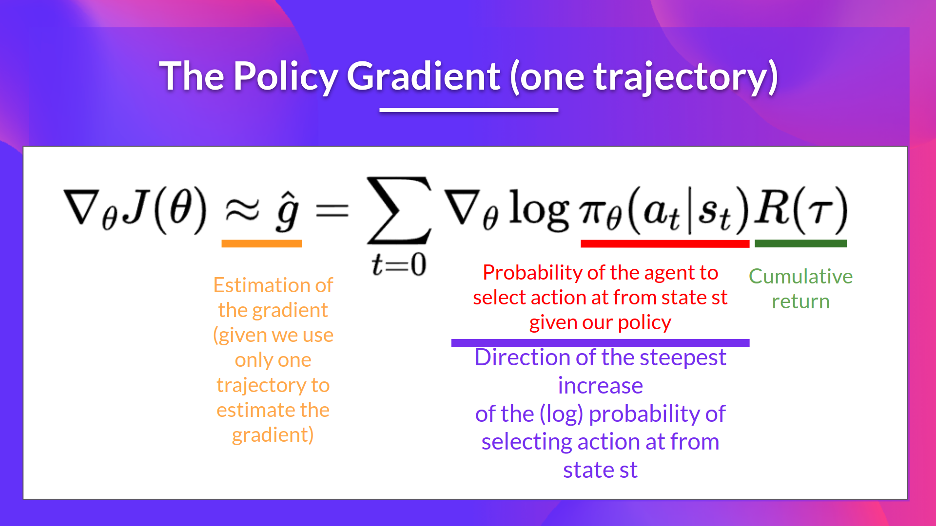
We can interpret this update as follows:

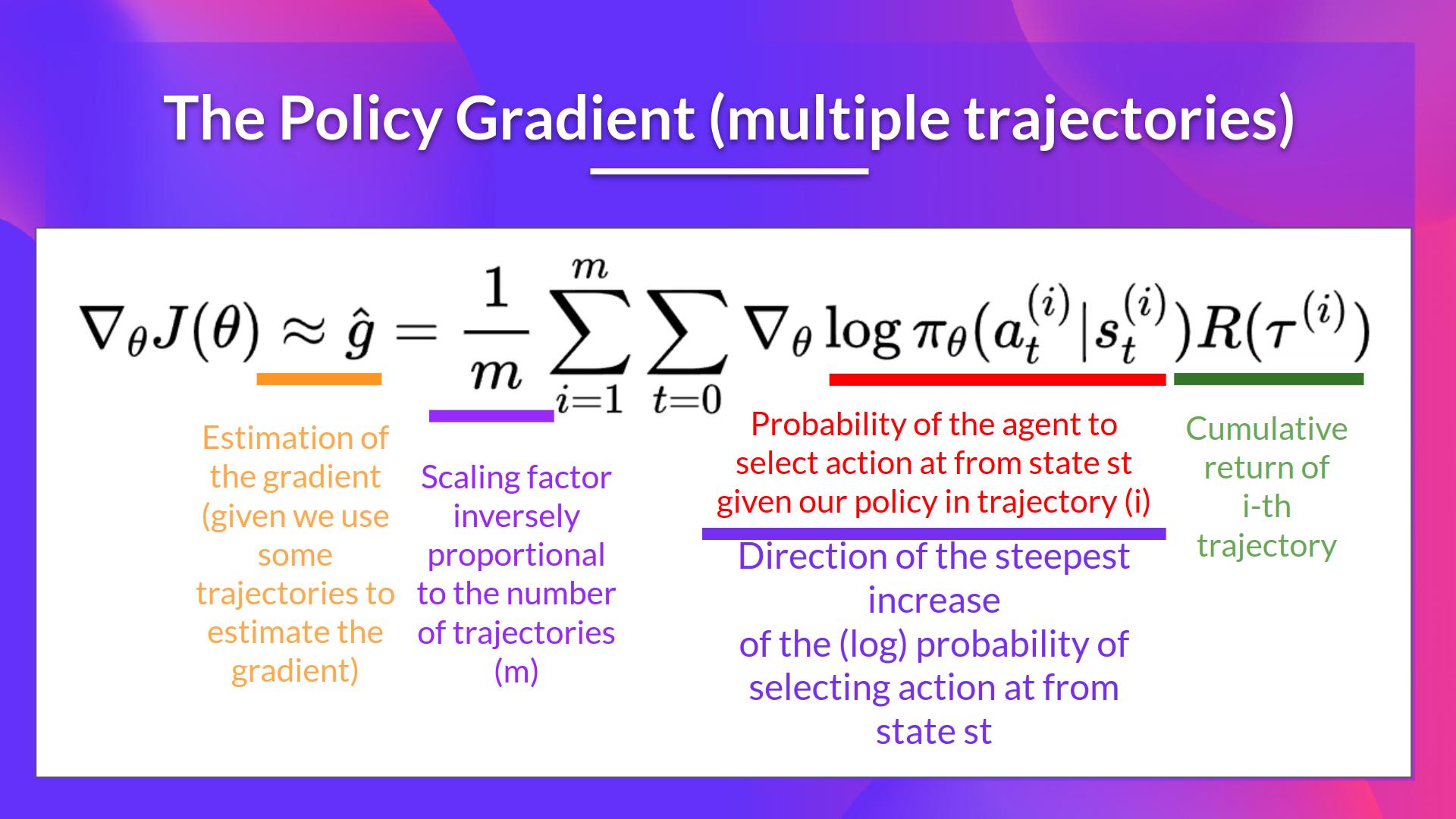
-$\nabla_\theta log \pi_\theta(a_t|s_t)$ is the direction of steepest increase of the (log) probability of selecting action$a_t$ from state$s_t$. This tells us how we should change the weights of policy if we want to increase/decrease the log probability of selecting action$a_t$ at state$s_t$.

-$R(\tau)$: is the scoring function:

• If the return is high, it will push up the probabilities of the (state, action) combinations.
• Otherwise, if the return is low, it will push down the probabilities of the (state, action) combinations.

We can also collect multiple episodes (trajectories) to estimate the gradient: