Deep RL Course documentation
Hands on
Hands on
Now that we’ve studied the theory behind Reinforce, you’re ready to code your Reinforce agent with PyTorch. And you’ll test its robustness using CartPole-v1 and PixelCopter,.
You’ll then be able to iterate and improve this implementation for more advanced environments.

To validate this hands-on for the certification process, you need to push your trained models to the Hub and:
- Get a result of >= 350 for
Cartpole-v1 - Get a result of >= 5 for
PixelCopter.
To find your result, go to the leaderboard and find your model, the result = mean_reward - std of reward. If you don’t see your model on the leaderboard, go at the bottom of the leaderboard page and click on the refresh button.
If you don’t find your model, go to the bottom of the page and click on the refresh button.
For more information about the certification process, check this section 👉 https://huggingface.co/deep-rl-course/en/unit0/introduction#certification-process
And you can check your progress here 👉 https://huggingface.co/spaces/ThomasSimonini/Check-my-progress-Deep-RL-Course
To start the hands-on click on Open In Colab button 👇 :
![]()
We strongly recommend students use Google Colab for the hands-on exercises instead of running them on their personal computers.
By using Google Colab, you can focus on learning and experimenting without worrying about the technical aspects of setting up your environments.
Unit 4: Code your first Deep Reinforcement Learning Algorithm with PyTorch: Reinforce. And test its robustness 💪

In this notebook, you’ll code your first Deep Reinforcement Learning algorithm from scratch: Reinforce (also called Monte Carlo Policy Gradient).
Reinforce is a Policy-based method: a Deep Reinforcement Learning algorithm that tries to optimize the policy directly without using an action-value function.
More precisely, Reinforce is a Policy-gradient method, a subclass of Policy-based methods that aims to optimize the policy directly by estimating the weights of the optimal policy using gradient ascent.
To test its robustness, we’re going to train it in 2 different simple environments:
- Cartpole-v1
- PixelcopterEnv
⬇️ Here is an example of what you will achieve at the end of this notebook. ⬇️
🎮 Environments:
📚 RL-Library:
- Python
- PyTorch
We’re constantly trying to improve our tutorials, so if you find some issues in this notebook, please open an issue on the GitHub Repo.
Objectives of this notebook 🏆
At the end of the notebook, you will:
- Be able to code a Reinforce algorithm from scratch using PyTorch.
- Be able to test the robustness of your agent using simple environments.
- Be able to push your trained agent to the Hub with a nice video replay and an evaluation score 🔥.
Prerequisites 🏗️
Before diving into the notebook, you need to:
🔲 📚 Study Policy Gradients by reading Unit 4
Let’s code Reinforce algorithm from scratch 🔥
Some advice 💡
It’s better to run this colab in a copy on your Google Drive, so that if it times out you still have the saved notebook on your Google Drive and do not need to fill everything in from scratch.
To do that you can either do Ctrl + S or File > Save a copy in Google Drive.
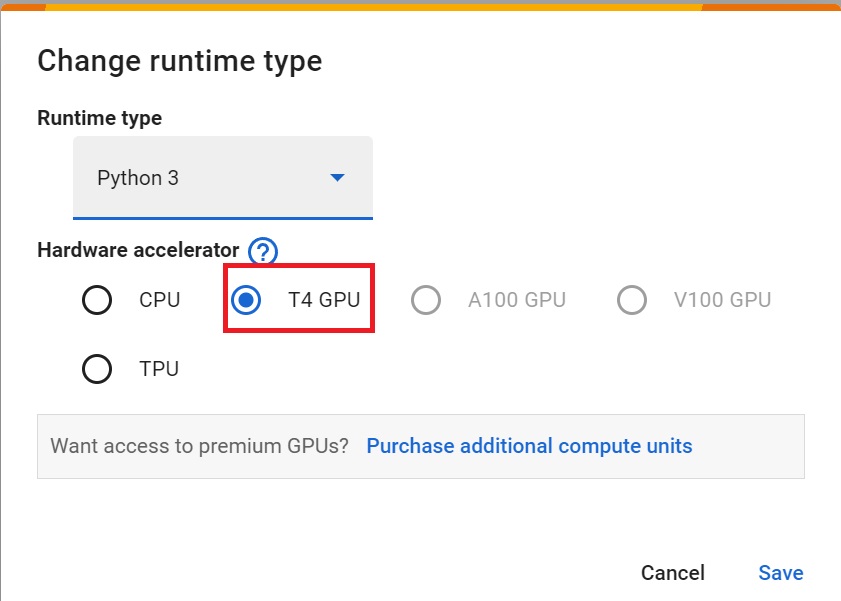
Set the GPU 💪
- To accelerate the agent’s training, we’ll use a GPU. To do that, go to
Runtime > Change Runtime type
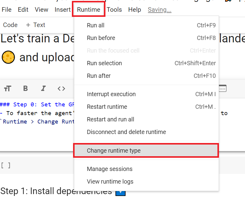
Hardware Accelerator > GPU
Create a virtual display 🖥
During the notebook, we’ll need to generate a replay video. To do so, with colab, we need to have a virtual screen to be able to render the environment (and thus record the frames).
The following cell will install the librairies and create and run a virtual screen 🖥
%%capture
!apt install python-opengl
!apt install ffmpeg
!apt install xvfb
!pip install pyvirtualdisplay
!pip install pyglet==1.5.1# Virtual display
from pyvirtualdisplay import Display
virtual_display = Display(visible=0, size=(1400, 900))
virtual_display.start()Install the dependencies 🔽
The first step is to install the dependencies. We’ll install multiple ones:
gymgym-games: Extra gym environments made with PyGame.huggingface_hub: The Hub works as a central place where anyone can share and explore models and datasets. It has versioning, metrics, visualizations, and other features that will allow you to easily collaborate with others.
You may be wondering why we install gym and not gymnasium, a more recent version of gym? Because the gym-games we are using are not updated yet with gymnasium.
The differences you’ll encounter here:
- In
gymwe don’t haveterminatedandtruncatedbut onlydone. - In
gymusingenv.step()returnsstate, reward, done, info
You can learn more about the differences between Gym and Gymnasium here 👉 https://gymnasium.farama.org/content/migration-guide/
You can see here all the Reinforce models available 👉 https://huggingface.co/models?other=reinforce
And you can find all the Deep Reinforcement Learning models here 👉 https://huggingface.co/models?pipeline_tag=reinforcement-learning
!pip install -r https://raw.githubusercontent.com/huggingface/deep-rl-class/main/notebooks/unit4/requirements-unit4.txt
Import the packages 📦
In addition to importing the installed libraries, we also import:
imageio: A library that will help us to generate a replay video
import numpy as np

from collections import deque

import matplotlib.pyplot as plt
%matplotlib inline

# PyTorch
import torch
import torch.nn as nn
import torch.nn.functional as F
import torch.optim as optim
from torch.distributions import Categorical

# Gym
import gym
import gym_pygame

# Hugging Face Hub
from huggingface_hub import notebook_login # To log to our Hugging Face account to be able to upload models to the Hub.
import imageio
Check if we have a GPU
- Let’s check if we have a GPU
- If it’s the case you should see
device:cuda0
device = torch.device("cuda:0" if torch.cuda.is_available() else "cpu")print(device)We’re now ready to implement our Reinforce algorithm 🔥
First agent: Playing CartPole-v1 🤖
Create the CartPole environment and understand how it works
The environment 🎮
Why do we use a simple environment like CartPole-v1?
As explained in Reinforcement Learning Tips and Tricks, when you implement your agent from scratch, you need to be sure that it works correctly and find bugs with easy environments before going deeper as finding bugs will be much easier in simple environments.
Try to have some “sign of life” on toy problems
Validate the implementation by making it run on harder and harder envs (you can compare results against the RL zoo). You usually need to run hyperparameter optimization for that step.
The CartPole-v1 environment
A pole is attached by an un-actuated joint to a cart, which moves along a frictionless track. The pendulum is placed upright on the cart and the goal is to balance the pole by applying forces in the left and right direction on the cart.
So, we start with CartPole-v1. The goal is to push the cart left or right so that the pole stays in the equilibrium.
The episode ends if:
- The pole Angle is greater than ±12°
- The Cart Position is greater than ±2.4
- The episode length is greater than 500
We get a reward 💰 of +1 every timestep that the Pole stays in the equilibrium.
env_id = "CartPole-v1"
# Create the env
env = gym.make(env_id)

# Create the evaluation env
eval_env = gym.make(env_id)

# Get the state space and action space
s_size = env.observation_space.shape[0]
a_size = env.action_space.nprint("_____OBSERVATION SPACE_____ \n")
print("The State Space is: ", s_size)
print("Sample observation", env.observation_space.sample()) # Get a random observationprint("\n _____ACTION SPACE_____ \n")
print("The Action Space is: ", a_size)
print("Action Space Sample", env.action_space.sample()) # Take a random actionLet’s build the Reinforce Architecture
This implementation is based on three implementations:
- PyTorch official Reinforcement Learning example
- Udacity Reinforce
- Improvement of the integration by Chris1nexus
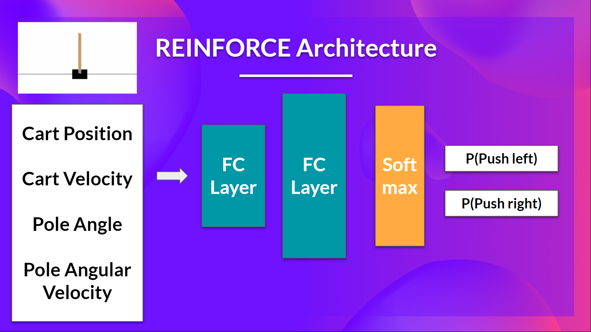
So we want:
- Two fully connected layers (fc1 and fc2).
- To use ReLU as activation function of fc1
- To use Softmax to output a probability distribution over actions
class Policy(nn.Module):
    def __init__(self, s_size, a_size, h_size):
        super(Policy, self).__init__()
        # Create two fully connected layers


    def forward(self, x):
        # Define the forward pass
        # state goes to fc1 then we apply ReLU activation function

        # fc1 outputs goes to fc2

        # We output the softmax

    def act(self, state):
        """
        Given a state, take action
        """
        state = torch.from_numpy(state).float().unsqueeze(0).to(device)
        probs = self.forward(state).cpu()
        m = Categorical(probs)
        action = np.argmax(m)
        return action.item(), m.log_prob(action)
Solution
class Policy(nn.Module):
    def __init__(self, s_size, a_size, h_size):
        super(Policy, self).__init__()
        self.fc1 = nn.Linear(s_size, h_size)
        self.fc2 = nn.Linear(h_size, a_size)

    def forward(self, x):
        x = F.relu(self.fc1(x))
        x = self.fc2(x)
        return F.softmax(x, dim=1)

    def act(self, state):
        state = torch.from_numpy(state).float().unsqueeze(0).to(device)
        probs = self.forward(state).cpu()
        m = Categorical(probs)
        action = np.argmax(m)
        return action.item(), m.log_prob(action)
I made a mistake, can you guess where?
- To find out let’s make a forward pass:
debug_policy = Policy(s_size, a_size, 64).to(device)
debug_policy.act(env.reset())
Here we see that the error says
ValueError: The value argument to log_prob must be a TensorIt means that
actioninm.log_prob(action)must be a Tensor but it’s not.Do you know why? Check the act function and try to see why it does not work.
Advice 💡: Something is wrong in this implementation. Remember that for the act function we want to sample an action from the probability distribution over actions.
(Real) Solution
class Policy(nn.Module):
    def __init__(self, s_size, a_size, h_size):
        super(Policy, self).__init__()
        self.fc1 = nn.Linear(s_size, h_size)
        self.fc2 = nn.Linear(h_size, a_size)

    def forward(self, x):
        x = F.relu(self.fc1(x))
        x = self.fc2(x)
        return F.softmax(x, dim=1)

    def act(self, state):
        state = torch.from_numpy(state).float().unsqueeze(0).to(device)
        probs = self.forward(state).cpu()
        m = Categorical(probs)
        action = m.sample()
        return action.item(), m.log_prob(action)
By using CartPole, it was easier to debug since we know that the bug comes from our integration and not from our simple environment.
Since we want to sample an action from the probability distribution over actions, we can’t use
action = np.argmax(m)since it will always output the action that has the highest probability.We need to replace this with
action = m.sample()which will sample an action from the probability distribution P(.|s)
Let’s build the Reinforce Training Algorithm
This is the Reinforce algorithm pseudocode:
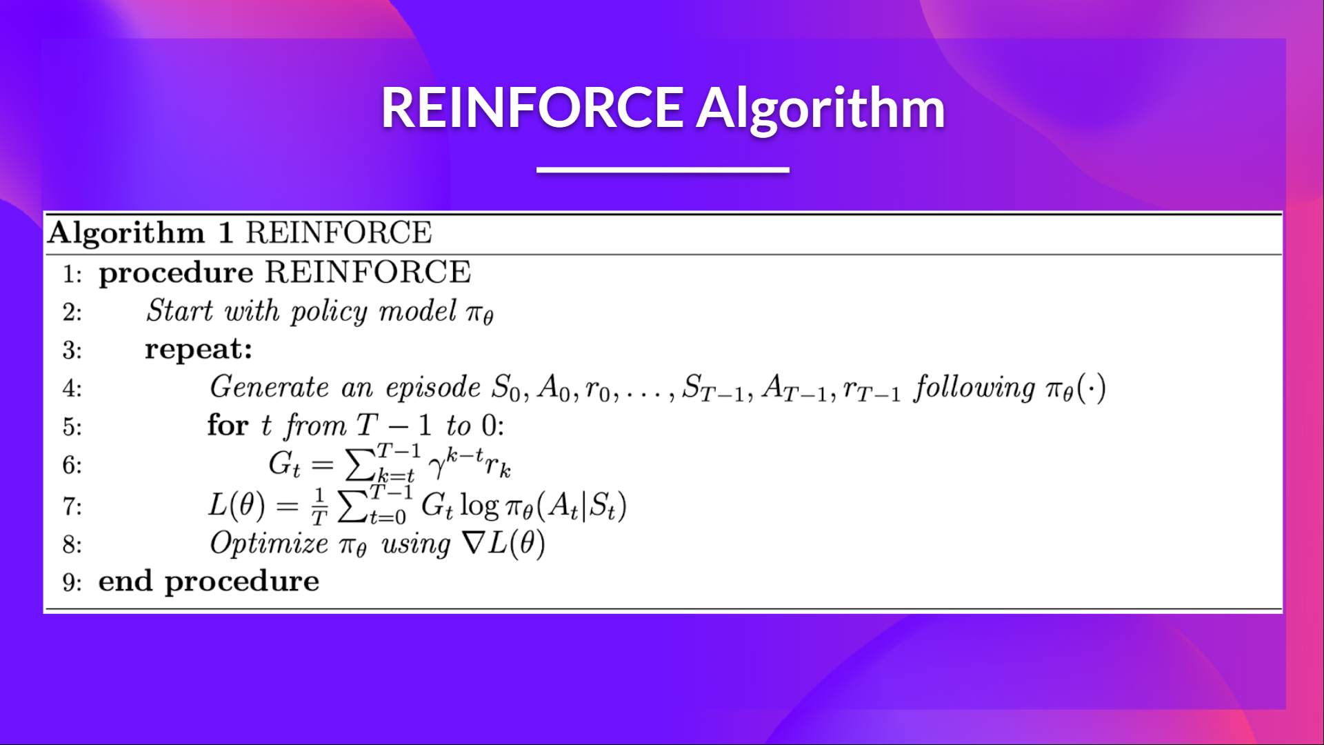
When we calculate the return Gt (line 6), we see that we calculate the sum of discounted rewards starting at timestep t.
Why? Because our policy should only reinforce actions on the basis of the consequences: so rewards obtained before taking an action are useless (since they were not because of the action), only the ones that come after the action matters.
Before coding this you should read this section don’t let the past distract you that explains why we use reward-to-go policy gradient.
We use an interesting technique coded by Chris1nexus to compute the return at each timestep efficiently. The comments explained the procedure. Don’t hesitate also to check the PR explanation But overall the idea is to compute the return at each timestep efficiently.
The second question you may ask is why do we minimize the loss? Didn’t we talk about Gradient Ascent, not Gradient Descent earlier?
- We want to maximize our utility function $J(\theta)$, but in PyTorch and TensorFlow, it’s better to minimize an objective function.
- So let’s say we want to reinforce action 3 at a certain timestep. Before training this action P is 0.25.
- So we want to modify such that
- Because all P must sum to 1, max will minimize other action probability.
- So we should tell PyTorch to min.
- This loss function approaches 0 as nears 1.
- So we are encouraging the gradient to max
def reinforce(policy, optimizer, n_training_episodes, max_t, gamma, print_every):
    # Help us to calculate the score during the training
    scores_deque = deque(maxlen=100)
    scores = []
    # Line 3 of pseudocode
    for i_episode in range(1, n_training_episodes+1):
        saved_log_probs = []
        rewards = []
        state = # TODO: reset the environment
        # Line 4 of pseudocode
        for t in range(max_t):
            action, log_prob = # TODO get the action
            saved_log_probs.append(log_prob)
            state, reward, done, _ = # TODO: take an env step
            rewards.append(reward)
            if done:
                break
        scores_deque.append(sum(rewards))
        scores.append(sum(rewards))

        # Line 6 of pseudocode: calculate the return
        returns = deque(maxlen=max_t)
        n_steps = len(rewards)
        # Compute the discounted returns at each timestep,
        # as the sum of the gamma-discounted return at time t (G_t) + the reward at time t

        # In O(N) time, where N is the number of time steps
        # (this definition of the discounted return G_t follows the definition of this quantity
        # shown at page 44 of Sutton&Barto 2017 2nd draft)
        # G_t = r_(t+1) + r_(t+2) + ...

        # Given this formulation, the returns at each timestep t can be computed
        # by re-using the computed future returns G_(t+1) to compute the current return G_t
        # G_t = r_(t+1) + gamma*G_(t+1)
        # G_(t-1) = r_t + gamma* G_t
        # (this follows a dynamic programming approach, with which we memorize solutions in order
        # to avoid computing them multiple times)

        # This is correct since the above is equivalent to (see also page 46 of Sutton&Barto 2017 2nd draft)
        # G_(t-1) = r_t + gamma*r_(t+1) + gamma*gamma*r_(t+2) + ...


        ## Given the above, we calculate the returns at timestep t as:
        #               gamma[t] * return[t] + reward[t]
        #
        ## We compute this starting from the last timestep to the first, in order
        ## to employ the formula presented above and avoid redundant computations that would be needed
        ## if we were to do it from first to last.

        ## Hence, the queue "returns" will hold the returns in chronological order, from t=0 to t=n_steps
        ## thanks to the appendleft() function which allows to append to the position 0 in constant time O(1)
        ## a normal python list would instead require O(N) to do this.
        for t in range(n_steps)[::-1]:
            disc_return_t = (returns[0] if len(returns)>0 else 0)
            returns.appendleft(    ) # TODO: complete here

        ## standardization of the returns is employed to make training more stable
        eps = np.finfo(np.float32).eps.item()

        ## eps is the smallest representable float, which is
        # added to the standard deviation of the returns to avoid numerical instabilities
        returns = torch.tensor(returns)
        returns = (returns - returns.mean()) / (returns.std() + eps)

        # Line 7:
        policy_loss = []
        for log_prob, disc_return in zip(saved_log_probs, returns):
            policy_loss.append(-log_prob * disc_return)
        policy_loss = torch.cat(policy_loss).sum()

        # Line 8: PyTorch prefers gradient descent
        optimizer.zero_grad()
        policy_loss.backward()
        optimizer.step()

        if i_episode % print_every == 0:
            print('Episode {}\tAverage Score: {:.2f}'.format(i_episode, np.mean(scores_deque)))

    return scores
Solution
def reinforce(policy, optimizer, n_training_episodes, max_t, gamma, print_every):
    # Help us to calculate the score during the training
    scores_deque = deque(maxlen=100)
    scores = []
    # Line 3 of pseudocode
    for i_episode in range(1, n_training_episodes + 1):
        saved_log_probs = []
        rewards = []
        state = env.reset()
        # Line 4 of pseudocode
        for t in range(max_t):
            action, log_prob = policy.act(state)
            saved_log_probs.append(log_prob)
            state, reward, done, _ = env.step(action)
            rewards.append(reward)
            if done:
                break
        scores_deque.append(sum(rewards))
        scores.append(sum(rewards))

        # Line 6 of pseudocode: calculate the return
        returns = deque(maxlen=max_t)
        n_steps = len(rewards)
        # Compute the discounted returns at each timestep,
        # as
        #      the sum of the gamma-discounted return at time t (G_t) + the reward at time t
        #
        # In O(N) time, where N is the number of time steps
        # (this definition of the discounted return G_t follows the definition of this quantity
        # shown at page 44 of Sutton&Barto 2017 2nd draft)
        # G_t = r_(t+1) + r_(t+2) + ...

        # Given this formulation, the returns at each timestep t can be computed
        # by re-using the computed future returns G_(t+1) to compute the current return G_t
        # G_t = r_(t+1) + gamma*G_(t+1)
        # G_(t-1) = r_t + gamma* G_t
        # (this follows a dynamic programming approach, with which we memorize solutions in order
        # to avoid computing them multiple times)

        # This is correct since the above is equivalent to (see also page 46 of Sutton&Barto 2017 2nd draft)
        # G_(t-1) = r_t + gamma*r_(t+1) + gamma*gamma*r_(t+2) + ...

        ## Given the above, we calculate the returns at timestep t as:
        #               gamma[t] * return[t] + reward[t]
        #
        ## We compute this starting from the last timestep to the first, in order
        ## to employ the formula presented above and avoid redundant computations that would be needed
        ## if we were to do it from first to last.

        ## Hence, the queue "returns" will hold the returns in chronological order, from t=0 to t=n_steps
        ## thanks to the appendleft() function which allows to append to the position 0 in constant time O(1)
        ## a normal python list would instead require O(N) to do this.
        for t in range(n_steps)[::-1]:
            disc_return_t = returns[0] if len(returns) > 0 else 0
            returns.appendleft(gamma * disc_return_t + rewards[t])

        ## standardization of the returns is employed to make training more stable
        eps = np.finfo(np.float32).eps.item()
        ## eps is the smallest representable float, which is
        # added to the standard deviation of the returns to avoid numerical instabilities
        returns = torch.tensor(returns)
        returns = (returns - returns.mean()) / (returns.std() + eps)

        # Line 7:
        policy_loss = []
        for log_prob, disc_return in zip(saved_log_probs, returns):
            policy_loss.append(-log_prob * disc_return)
        policy_loss = torch.cat(policy_loss).sum()

        # Line 8: PyTorch prefers gradient descent
        optimizer.zero_grad()
        policy_loss.backward()
        optimizer.step()

        if i_episode % print_every == 0:
            print("Episode {}\tAverage Score: {:.2f}".format(i_episode, np.mean(scores_deque)))

    return scores
Train it
- We’re now ready to train our agent.
- But first, we define a variable containing all the training hyperparameters.
- You can change the training parameters (and should 😉)
cartpole_hyperparameters = {
    "h_size": 16,
    "n_training_episodes": 1000,
    "n_evaluation_episodes": 10,
    "max_t": 1000,
    "gamma": 1.0,
    "lr": 1e-2,
    "env_id": env_id,
    "state_space": s_size,
    "action_space": a_size,
}# Create policy and place it to the device
cartpole_policy = Policy(
cartpole_hyperparameters["state_space"],
cartpole_hyperparameters["action_space"],
cartpole_hyperparameters["h_size"],
).to(device)
cartpole_optimizer = optim.Adam(cartpole_policy.parameters(), lr=cartpole_hyperparameters["lr"])scores = reinforce(
cartpole_policy,
cartpole_optimizer,
cartpole_hyperparameters["n_training_episodes"],
cartpole_hyperparameters["max_t"],
cartpole_hyperparameters["gamma"],
100,
)Define evaluation method 📝
- Here we define the evaluation method that we’re going to use to test our Reinforce agent.
def evaluate_agent(env, max_steps, n_eval_episodes, policy):
    """
    Evaluate the agent for ``n_eval_episodes`` episodes and returns average reward and std of reward.
    :param env: The evaluation environment
    :param n_eval_episodes: Number of episode to evaluate the agent
    :param policy: The Reinforce agent
    """
    episode_rewards = []
    for episode in range(n_eval_episodes):
        state = env.reset()
        step = 0
        done = False
        total_rewards_ep = 0

        for step in range(max_steps):
            action, _ = policy.act(state)
            new_state, reward, done, info = env.step(action)
            total_rewards_ep += reward

            if done:
                break
            state = new_state
        episode_rewards.append(total_rewards_ep)
    mean_reward = np.mean(episode_rewards)
    std_reward = np.std(episode_rewards)

    return mean_reward, std_reward
Evaluate our agent 📈
evaluate_agent(
    eval_env, cartpole_hyperparameters["max_t"], cartpole_hyperparameters["n_evaluation_episodes"], cartpole_policy
)
Publish our trained model on the Hub 🔥
Now that we saw we got good results after the training, we can publish our trained model on the hub 🤗 with one line of code.
Here’s an example of a Model Card:

Push to the Hub
Do not modify this code
from huggingface_hub import HfApi, snapshot_download
from huggingface_hub.repocard import metadata_eval_result, metadata_save

from pathlib import Path
import datetime
import json
import imageio

import tempfile

import osdef record_video(env, policy, out_directory, fps=30):
"""
Generate a replay video of the agent
:param env
:param Qtable: Qtable of our agent
:param out_directory
:param fps: how many frame per seconds (with taxi-v3 and frozenlake-v1 we use 1)
"""
images = []
done = False
state = env.reset()
img = env.render(mode="rgb_array")
images.append(img)
while not done:
# Take the action (index) that have the maximum expected future reward given that state
action, _ = policy.act(state)
state, reward, done, info = env.step(action) # We directly put next_state = state for recording logic
img = env.render(mode="rgb_array")
images.append(img)
imageio.mimsave(out_directory, [np.array(img) for i, img in enumerate(images)], fps=fps)def push_to_hub(repo_id,
model,
hyperparameters,
eval_env,
video_fps=30
):
"""
Evaluate, Generate a video and Upload a model to Hugging Face Hub.
This method does the complete pipeline:
- It evaluates the model
- It generates the model card
- It generates a replay video of the agent
- It pushes everything to the Hub
:param repo_id: repo_id: id of the model repository from the Hugging Face Hub
:param model: the pytorch model we want to save
:param hyperparameters: training hyperparameters
:param eval_env: evaluation environment
:param video_fps: how many frame per seconds to record our video replay
"""
_, repo_name = repo_id.split("/")
api = HfApi()
# Step 1: Create the repo
repo_url = api.create_repo(
repo_id=repo_id,
exist_ok=True,
)
with tempfile.TemporaryDirectory() as tmpdirname:
local_directory = Path(tmpdirname)
# Step 2: Save the model
torch.save(model, local_directory / "model.pt")
# Step 3: Save the hyperparameters to JSON
with open(local_directory / "hyperparameters.json", "w") as outfile:
json.dump(hyperparameters, outfile)
# Step 4: Evaluate the model and build JSON
mean_reward, std_reward = evaluate_agent(eval_env,
hyperparameters["max_t"],
hyperparameters["n_evaluation_episodes"],
model)
# Get datetime
eval_datetime = datetime.datetime.now()
eval_form_datetime = eval_datetime.isoformat()
evaluate_data = {
"env_id": hyperparameters["env_id"],
"mean_reward": mean_reward,
"n_evaluation_episodes": hyperparameters["n_evaluation_episodes"],
"eval_datetime": eval_form_datetime,
}
# Write a JSON file
with open(local_directory / "results.json", "w") as outfile:
json.dump(evaluate_data, outfile)
# Step 5: Create the model card
env_name = hyperparameters["env_id"]
metadata = {}
metadata["tags"] = [
env_name,
"reinforce",
"reinforcement-learning",
"custom-implementation",
"deep-rl-class"
]
# Add metrics
eval = metadata_eval_result(
model_pretty_name=repo_name,
task_pretty_name="reinforcement-learning",
task_id="reinforcement-learning",
metrics_pretty_name="mean_reward",
metrics_id="mean_reward",
metrics_value=f"{mean_reward:.2f} +/- {std_reward:.2f}",
dataset_pretty_name=env_name,
dataset_id=env_name,
)
# Merges both dictionaries
metadata = {**metadata, **eval}
model_card = f"""
# **Reinforce** Agent playing **{env_id}**
This is a trained model of a **Reinforce** agent playing **{env_id}** .
To learn to use this model and train yours check Unit 4 of the Deep Reinforcement Learning Course: https://huggingface.co/deep-rl-course/unit4/introduction
"""
readme_path = local_directory / "README.md"
readme = ""
if readme_path.exists():
with readme_path.open("r", encoding="utf8") as f:
readme = f.read()
else:
readme = model_card
with readme_path.open("w", encoding="utf-8") as f:
f.write(readme)
# Save our metrics to Readme metadata
metadata_save(readme_path, metadata)
# Step 6: Record a video
video_path = local_directory / "replay.mp4"
record_video(env, model, video_path, video_fps)
# Step 7. Push everything to the Hub
api.upload_folder(
repo_id=repo_id,
folder_path=local_directory,
path_in_repo=".",
)
print(f"Your model is pushed to the Hub. You can view your model here: {repo_url}")By using push_to_hub, you evaluate, record a replay, generate a model card of your agent, and push it to the Hub.
This way:
- You can showcase our work 🔥
- You can visualize your agent playing 👀
- You can share an agent with the community that others can use 💾
- You can access a leaderboard 🏆 to see how well your agent is performing compared to your classmates 👉 https://huggingface.co/spaces/huggingface-projects/Deep-Reinforcement-Learning-Leaderboard
To be able to share your model with the community there are three more steps to follow:
1️⃣ (If it’s not already done) create an account to HF ➡ https://huggingface.co/join
2️⃣ Sign in and then, you need to store your authentication token from the Hugging Face website.
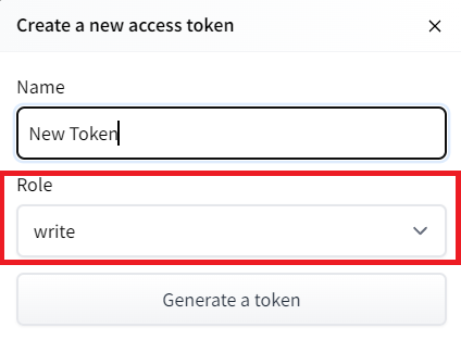
- Create a new token (https://huggingface.co/settings/tokens) with write role
notebook_login()
If you don’t want to use Google Colab or a Jupyter Notebook, you need to use this command instead: huggingface-cli login (or login)
3️⃣ We’re now ready to push our trained agent to the 🤗 Hub 🔥 using package_to_hub() function
repo_id = ""  # TODO Define your repo id {username/Reinforce-{model-id}}
push_to_hub(
    repo_id,
    cartpole_policy,  # The model we want to save
    cartpole_hyperparameters,  # Hyperparameters
    eval_env,  # Evaluation environment
    video_fps=30
)
Now that we tested the robustness of our implementation, let’s try a more complex environment: PixelCopter 🚁
Second agent: PixelCopter 🚁
Study the PixelCopter environment 👀
env_id = "Pixelcopter-PLE-v0"
env = gym.make(env_id)
eval_env = gym.make(env_id)
s_size = env.observation_space.shape[0]
a_size = env.action_space.nprint("_____OBSERVATION SPACE_____ \n")
print("The State Space is: ", s_size)
print("Sample observation", env.observation_space.sample()) # Get a random observationprint("\n _____ACTION SPACE_____ \n")
print("The Action Space is: ", a_size)
print("Action Space Sample", env.action_space.sample()) # Take a random actionThe observation space (7) 👀:
- player y position
- player velocity
- player distance to floor
- player distance to ceiling
- next block x distance to player
- next blocks top y location
- next blocks bottom y location
The action space(2) 🎮:
- Up (press accelerator)
- Do nothing (don’t press accelerator)
The reward function 💰:
- For each vertical block it passes, it gains a positive reward of +1. Each time a terminal state is reached it receives a negative reward of -1.
Define the new Policy 🧠
- We need to have a deeper neural network since the environment is more complex
class Policy(nn.Module):
    def __init__(self, s_size, a_size, h_size):
        super(Policy, self).__init__()
        # Define the three layers here

    def forward(self, x):
        # Define the forward process here
        return F.softmax(x, dim=1)

    def act(self, state):
        state = torch.from_numpy(state).float().unsqueeze(0).to(device)
        probs = self.forward(state).cpu()
        m = Categorical(probs)
        action = m.sample()
        return action.item(), m.log_prob(action)
Solution
class Policy(nn.Module):
    def __init__(self, s_size, a_size, h_size):
        super(Policy, self).__init__()
        self.fc1 = nn.Linear(s_size, h_size)
        self.fc2 = nn.Linear(h_size, h_size * 2)
        self.fc3 = nn.Linear(h_size * 2, a_size)

    def forward(self, x):
        x = F.relu(self.fc1(x))
        x = F.relu(self.fc2(x))
        x = self.fc3(x)
        return F.softmax(x, dim=1)

    def act(self, state):
        state = torch.from_numpy(state).float().unsqueeze(0).to(device)
        probs = self.forward(state).cpu()
        m = Categorical(probs)
        action = m.sample()
        return action.item(), m.log_prob(action)
Define the hyperparameters ⚙️
- Because this environment is more complex.
- Especially for the hidden size, we need more neurons.
pixelcopter_hyperparameters = {
    "h_size": 64,
    "n_training_episodes": 50000,
    "n_evaluation_episodes": 10,
    "max_t": 10000,
    "gamma": 0.99,
    "lr": 1e-4,
    "env_id": env_id,
    "state_space": s_size,
    "action_space": a_size,
}
Train it
- We’re now ready to train our agent 🔥.
# Create policy and place it to the device
# torch.manual_seed(50)
pixelcopter_policy = Policy(
    pixelcopter_hyperparameters["state_space"],
    pixelcopter_hyperparameters["action_space"],
    pixelcopter_hyperparameters["h_size"],
).to(device)
pixelcopter_optimizer = optim.Adam(pixelcopter_policy.parameters(), lr=pixelcopter_hyperparameters["lr"])scores = reinforce(
pixelcopter_policy,
pixelcopter_optimizer,
pixelcopter_hyperparameters["n_training_episodes"],
pixelcopter_hyperparameters["max_t"],
pixelcopter_hyperparameters["gamma"],
1000,
)Publish our trained model on the Hub 🔥
repo_id = ""  # TODO Define your repo id {username/Reinforce-{model-id}}
push_to_hub(
    repo_id,
    pixelcopter_policy,  # The model we want to save
    pixelcopter_hyperparameters,  # Hyperparameters
    eval_env,  # Evaluation environment
    video_fps=30
)
Some additional challenges 🏆
The best way to learn is to try things on your own! As you saw, the current agent is not doing great. As a first suggestion, you can train for more steps. But also try to find better parameters.
In the Leaderboard you will find your agents. Can you get to the top?
Here are some ideas to climb up the leaderboard:
- Train more steps
- Try different hyperparameters by looking at what your classmates have done 👉 https://huggingface.co/models?other=reinforce
- Push your new trained model on the Hub 🔥
- Improving the implementation for more complex environments (for instance, what about changing the network to a Convolutional Neural Network to handle frames as observation)?
Congrats on finishing this unit! There was a lot of information. And congrats on finishing the tutorial. You’ve just coded your first Deep Reinforcement Learning agent from scratch using PyTorch and shared it on the Hub 🥳.
Don’t hesitate to iterate on this unit by improving the implementation for more complex environments (for instance, what about changing the network to a Convolutional Neural Network to handle frames as observation)?
In the next unit, we’re going to learn more about Unity MLAgents, by training agents in Unity environments. This way, you will be ready to participate in the AI vs AI challenges where you’ll train your agents to compete against other agents in a snowball fight and a soccer game.
Sound fun? See you next time!
Finally, we would love to hear what you think of the course and how we can improve it. If you have some feedback then please 👉 fill this form
See you in Unit 5! 🔥