Europe Reanalysis Super Resolution
The aim of the project is to create a Machine learning (ML) model that can generate high-resolution regional reanalysis data (similar to the one produced by CERRA) by downscaling global reanalysis data from ERA5.
This will be accomplished by using state-of-the-art Deep Learning (DL) techniques like U-Net, conditional GAN, and diffusion models (among others). Additionally, an ingestion module will be implemented to assess the possible benefit of using CERRA pseudo-observations as extra predictors. Once the model is designed and trained, a detailed validation framework takes the place.
It combines classical deterministic error metrics with in-depth validations, including time series, maps, spatio-temporal correlations, and computer vision metrics, disaggregated by months, seasons, and geographical regions, to evaluate the effectiveness of the model in reducing errors and representing physical processes. This level of granularity allows for a more comprehensive and accurate assessment, which is critical for ensuring that the model is effective in practice.
Moreover, tools for interpretability of DL models can be used to understand the inner workings and decision-making processes of these complex structures by analyzing the activations of different neurons and the importance of different features in the input data.
This work is funded by Code for Earth 2023 initiative.
The denoise model is released in Apache 2.0, making it usable without restrictions anywhere.
Table of Contents
- Model Card for Europe Reanalysis Super Resolution
- Table of Contents
- Model Details
- Training Details
- Results
- Next Steps
- Compute Infrastructure
- Authors
Model Details
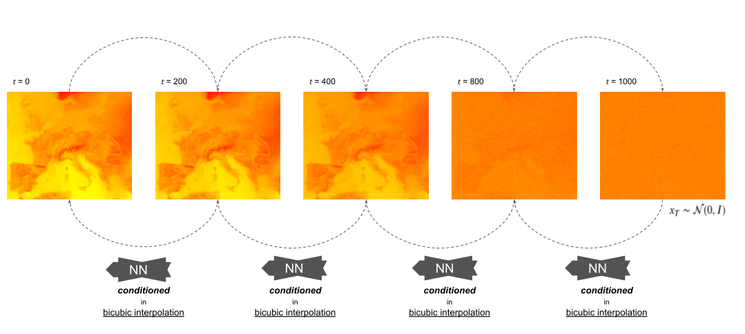
This model corresponds to a Denoise Neural Network trained with instance normalization over bicubic interpolated inputs.
We have implemented a diffusers.UNet2DModel for a Denoising Diffusion Probabilistic Model, with different schedulers: DDPMScheduler, DDIM and LMSDiscreteScheduler.
Model Description
We present the results of using Diffusion models (DM) for down-scaling (from 0.25º to 0.05º) regional reanalysis grids in the mediterranean area.
- Developed by: A team of Predictia Intelligent Data Solutions S.L.
- Model type: Vision model
- Language(s) (NLP): en, es
- License: Apache-2.0
- Resources for more information: More information needed
Denoise Network
For the Denoise network, we have only explored one architecture, diffusers.UNet2DModel, with differente model sizes, ranging from 3 blocks of 64, 128 and 192 out channels to the default configuration of 4 blocks of 224, 448, 672 and 896 out channels.
This network always takes:
- 2 channels as inputs corresponding to the noisy image at a timestep , and the bicubic upsampled ERA5 field.
- The timestep , which is projected to an embedding that is added to the input.
Noise Scheduler
Different schedulers have been considered.
Training Data
The dataset used is a composition of the ERA5 and CERRA reanalysis.
The spatial coverage of the input grids (ERA5) is defined below, and corresponds to a 2D array of dimensions (60, 42):
      longitude: [-8.35, 6.6]
      latitude: [46.45, 35.50]
On the other hand, the target high-resolution grid (CERRA) correspond to a 2D matrix of dimmension (240, 160):
      longitude: [-6.85, 5.1]
      latitude: [44.95, 37]
The data samples used for training corresponds to the period from 1981 and 2013 (both included) and from 2014 to 2017 for per-epoch validation.
Normalization techniques
All of these normalization techniques have been explored during and after ECMWF Code 4 Earth.
With monthly climatologies. This corresponds to compute the historical climatologies during the training period for each region (pixel or domain), and normalize with respect to that. In our case, the monthly climatologies are considered, but it could also be disaggregated by time of day, for example.
- Pixel-wise: In this case, the climatology is computed for each pixel of the meteorological field. Then, each pixel is standardized with its own climatology statistics.
- Domain-wise: Here, the climatology statistics are computed for the whole domain of interest. After computing the statistics, 2 normalizing schemas are possible:
- Independent: it refers to normalizing ERA5 and CERRA independently, each with its own statistics.
- Dependent: it refers to use only the climatology statistics from ERA5 to standardize both ERA5 and CERRA simultaneously.
The dependent approach is not feasible for the pixel-wise schema, because there is no direct correspondence between the input and output patch pixels. If we would be interested in doing so, there is the possibility to compute the statistics over the bicubic downsampled ERA5, and use those statistics for normalizing CERRA.
Without past information. This corresponds to normalizing each sample independently by the mean and standard deviation of the ERA5 field. This is known in the ML community as instance normalization. Here, we have to use only the distribution statistics from the inputs as the outputs will not be available during inference, but 2 different variations are possible in our use case:
- Use the statistics of the input ERA5. Recall that it covers a wider area than CERRA.
- Use the statistics of the bicubic downscaled ERA5, which represents the same area as CERRA.
The difference between these two approaches is not about calculating the statistics on the downscaled or source ERA5. The difference is that the input patch encompasses a larger area, and therefore a more different distribution. Thus, the second approach seems more correct as the downscaled area distribution will be more similar to the output distribution.
Results
The results of this model are NOT considered ACCEPTABLE, since they are not comparable with bicubic interpolation, a simple method which is also considered as input to the model. Therefore, although more complex tests are performed, such as including other covariates (e.g. time of day), they are not detailed here because their real effect on the performance of the model cannot be determined.
In this repository, we present the best performing Diffusion Model, which is trained with the scheduler specified at scheduler_config.json with the parameters shown in config.json and instance normalization over the downsampled ERA5 inputs.
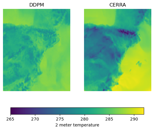
Below, the sample predicition of the 64M parameters Diffusion Model, with 1000 inference timesteps, at 00H of the January 1, 2018 compared with the CERRA reanalysis.
Normalization
- The pixel wise normalization does not make sense in this problem setup, as erases the spatial pattern and the DDPM is not able to learn anything.
- In contrast, when scaling with domain statistics the DDPM reproduce high resolution details that are not present in the input ERA5, but it fails to match the current high resolution field. The DDPM samples have appearance of CERRA-like fields, but when computing the MSE over a period is x3 larger than the bicubic interpolation.
- When scaling with domain statistics, using the same statistics for input and output represents slightly better the mean values of the predictions, but all fail to reproduce the variance of the field as seen in the sample.
- The instance normalization directly on the Denoise Network inputs (downsampled ERA5) reproduce slightly better the spatial pattern than others. The error metrics are more homogeneous spatially. For example, the spatial pattern of mountainous areas is very well reproduced.
Schedulers
There is no significant difference in trainining time, or sampling quality (at maximum capabilities). The difference between schedulers may arise during influence, when DDIM or LMSDiscrete may have higher quality samples with fewer inference steps, and consequently lower computational cost.
As satisfying performance is not reaching at maximum capabilities (inference steps = number training timesteps), therea has not been any research of the schedulers efficiency during sampling, which by the scientific literature may be sufficient with 40 samples (1/25 of the current inference timesteps).
Model sizes
This is strongly related to training time. Not only because of the time it takes to run the forward & backward process of the network, but also because of the limited memory available to load the samples, and then the need for more (smaller) batches to complete each epoch.
With the limited computational resources available, and the dataset considered, the tests carried out have indicated that there is an improvement when going from tens of output channels to a few hundred, obtaining networks of between 20 and 100 million parameters, but that it is not possible to reach the default size due to failures during training (i.e. gradient explosion, etc...).
Next steps
As this factors (model size, normalization and noise schedulers) have been extensively explored, it is necessary to move the research efforts to other aspects, as the followings:
Train a VAE, to work with Latent DM. This can be though as a learnable normalization with the additional advantage of reducing the sample size, and therefore the computational cost.
Train a larger denoise network. To this aim, it may be necessary a larger VM and/or training with more samples. For example, it may be beneficial to start learning with random patches (during the firsts epochs), and then fine-tune with the current domain the last epochs.
Another DM flavours, like Score Based DM.
Try new architecture availables in diffusers.
Based on scientific literature for other problems like Super Resolution in Computer Vision, where they work with larger samples -3 channels rather than 1, and more pixels- better results have to be achievable with this architecture type and DM flavour.
To tackle the most limiting factor, we think the best options are to explore options 1 and 2.
Compute Infrastructure
The use of GPUs in deep learning projects significantly accelerates model training and inference, leading to substantial reductions in computation time and making it feasible to tackle complex tasks and large datasets with efficiency.
The generosity and collaboration of our partners are instrumental to the success of this projects, significantly contributing to our research and development endeavors.
AI4EOSC: AI4EOSC stands for "Artificial Intelligence for the European Open Science Cloud." The European Open Science Cloud (EOSC) is a European Union initiative that aims to create a federated environment of research data and services. AI4EOSC is a specific project or initiative within the EOSC framework that focuses on the integration and application of artificial intelligence (AI) technologies in the context of open science.
European Weather Cloud: The European Weather Cloud is the cloud-based collaboration platform for meteorological application development and operations in Europe. Services provided range from delivery of weather forecast data and products to the provision of computing and storage resources, support and expert advice.
Hardware
For our project, we have deployed two virtual machines (VMs), each featuring a dedicated Graphics Processing Unit (GPU). One VM is equipped with a 16GB GPU, while the other boasts a more substantial 20GB GPU. This resource configuration allows us to efficiently manage a wide range of computing tasks, from data processing to model training, and ultimately drives the successful execution of our project.
Software
The code used to train and evaluate this model is freely available through its GitHub Repository ECMWFCode4Earth/DeepR hosted in the ECWMF Code 4 Earth organization.
Authors
Mario Santa Cruz. Predictia Intelligent Data Solutions S.L.
Antonio Pérez. Predictia Intelligent Data Solutions S.L.
Javier Díez. Predictia Intelligent Data Solutions S.L.
- Downloads last month
- 34

