Object Detection Leaderboard: Decoding Metrics and Their Potential Pitfalls


Welcome to our latest dive into the world of leaderboards and models evaluation. In a previous post, we navigated the waters of evaluating Large Language Models. Today, we set sail to a different, yet equally challenging domain – Object Detection.
Recently, we released our Object Detection Leaderboard, ranking object detection models available in the Hub according to some metrics. In this blog, we will demonstrate how the models were evaluated and demystify the popular metrics used in Object Detection, from Intersection over Union (IoU) to Average Precision (AP) and Average Recall (AR). More importantly, we will spotlight the inherent divergences and pitfalls that can occur during evaluation, ensuring that you're equipped with the knowledge not just to understand but to assess model performance critically.
Every developer and researcher aims for a model that can accurately detect and delineate objects. Our Object Detection Leaderboard is the right place to find an open-source model that best fits their application needs. But what does "accurate" truly mean in this context? Which metrics should one trust? How are they computed? And, perhaps more crucially, why some models may present divergent results in different reports? All these questions will be answered in this blog.
So, let's embark on this exploration together and unlock the secrets of the Object Detection Leaderboard! If you prefer to skip the introduction and learn how object detection metrics are computed, go to the Metrics section. If you wish to find how to pick the best models based on the Object Detection Leaderboard, you may check the Object Detection Leaderboard section.
Table of Contents
- Introduction
- What's Object Detection
- Metrics
- Object Detection Leaderboard
- Conclusions
- Additional Resources
What's Object Detection?
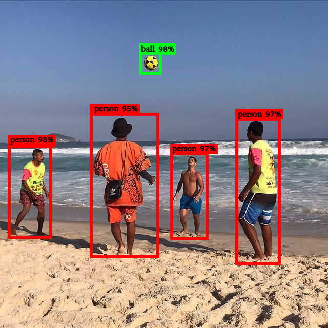
In the field of Computer Vision, Object Detection refers to the task of identifying and localizing individual objects within an image. Unlike image classification, where the task is to determine the predominant object or scene in the image, object detection not only categorizes the object classes present but also provides spatial information, drawing bounding boxes around each detected object. An object detector can also output a "score" (or "confidence") per detection. It represents the probability, according to the model, that the detected object belongs to the predicted class for each bounding box.
The following image, for instance, shows five detections: one "ball" with a confidence of 98% and four "person" with a confidence of 98%, 95%, 97%, and 97%.
Object detection models are versatile and have a wide range of applications across various domains. Some use cases include vision in autonomous vehicles, face detection, surveillance and security, medical imaging, augmented reality, sports analysis, smart cities, gesture recognition, etc.
The Hugging Face Hub has hundreds of object detection models pre-trained in different datasets, able to identify and localize various object classes.
One specific type of object detection models, called zero-shot, can receive additional text queries to search for target objects described in the text. These models can detect objects they haven't seen during training, instead of being constrained to the set of classes used during training.
The diversity of detectors goes beyond the range of output classes they can recognize. They vary in terms of underlying architectures, model sizes, processing speeds, and prediction accuracy.
A popular metric used to evaluate the accuracy of predictions made by an object detection model is the Average Precision (AP) and its variants, which will be explained later in this blog.
Evaluating an object detection model encompasses several components, like a dataset with ground-truth annotations, detections (output prediction), and metrics. This process is depicted in the schematic provided in Figure 2:
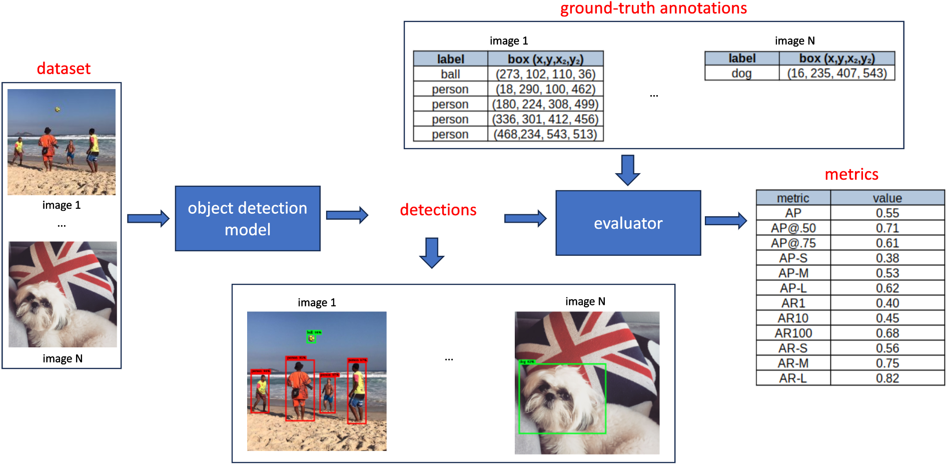
First, a benchmarking dataset containing images with ground-truth bounding box annotations is chosen and fed into the object detection model. The model predicts bounding boxes for each image, assigning associated class labels and confidence scores to each box. During the evaluation phase, these predicted bounding boxes are compared with the ground-truth boxes in the dataset. The evaluation yields a set of metrics, each ranging between [0, 1], reflecting a specific evaluation criteria. In the next section, we'll dive into the computation of the metrics in detail.
Metrics
This section will delve into the definition of Average Precision and Average Recall, their variations, and their associated computation methodologies.
What's Average Precision and how to compute it?
Average Precision (AP) is a single-number that summarizes the Precision x Recall curve. Before we explain how to compute it, we first need to understand the concept of Intersection over Union (IoU), and how to classify a detection as a True Positive or a False Positive.
IoU is a metric represented by a number between 0 and 1 that measures the overlap between the predicted bounding box and the actual (ground truth) bounding box. It's computed by dividing the area where the two boxes overlap by the area covered by both boxes combined. Figure 3 visually demonstrates the IoU using an example of a predicted box and its corresponding ground-truth box.
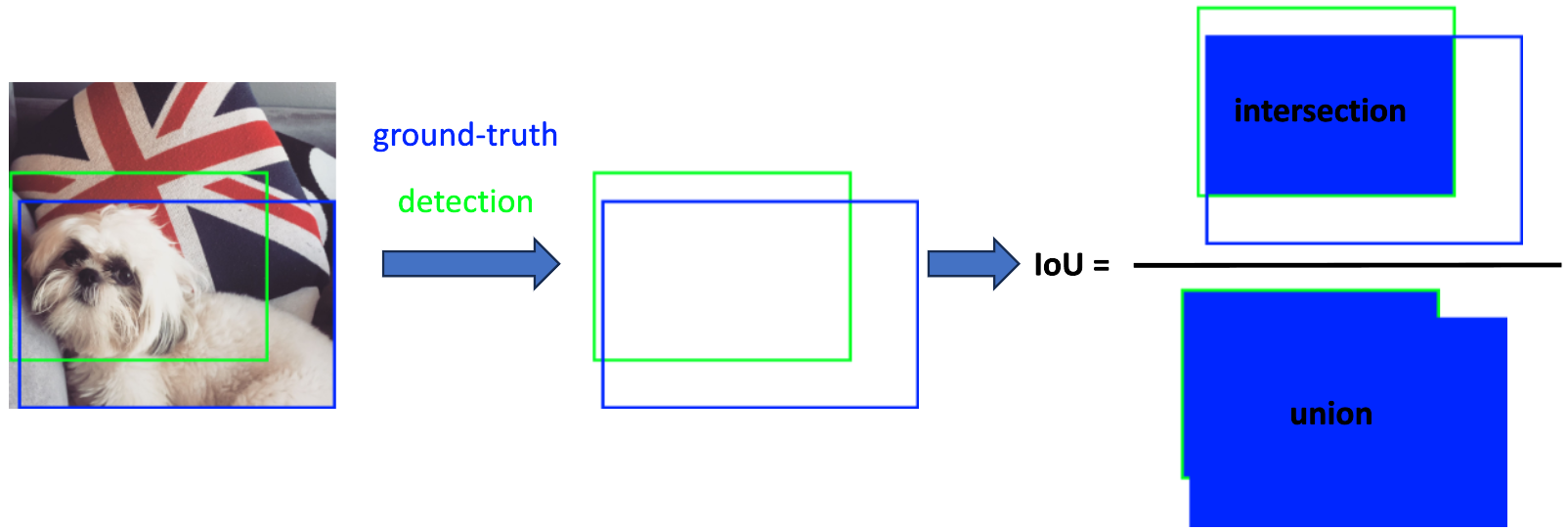
If the ground truth and detected boxes share identical coordinates, representing the same region in the image, their IoU value is 1. Conversely, if the boxes do not overlap at any pixel, the IoU is considered to be 0.
In scenarios where high precision in detections is expected (e.g. an autonomous vehicle), the predicted bounding boxes should closely align with the ground-truth boxes. For that, a IoU threshold ( ) approaching 1 is preferred. On the other hand, for applications where the exact position of the detected bounding boxes relative to the target object isn’t critical, the threshold can be relaxed, setting closer to 0.
Every box predicted by the model is considered a “positive” detection. The Intersection over Union (IoU) criterion classifies each prediction as a true positive (TP) or a false positive (FP), according to the confidence threshold we defined.
Based on predefined , we can define True Positives and True Negatives:
- True Positive (TP): A correct detection where IoU ≥ .
- False Positive (FP): An incorrect detection (missed object), where the IoU < .
Conversely, negatives are evaluated based on a ground-truth bounding box and can be defined as False Negative (FN) or True Negative (TN):
- False Negative (FN): Refers to a ground-truth object that the model failed to detect.
- True Negative (TN): Denotes a correct non-detection. Within the domain of object detection, countless bounding boxes within an image should NOT be identified, as they don't represent the target object. Consider all possible boxes in an image that don’t represent the target object - quite a vast number, isn’t it? :) That's why we do not consider TN to compute object detection metrics.
Now that we can identify our TPs, FPs, and FNs, we can define Precision and Recall:
- Precision is the ability of a model to identify only the relevant objects. It is the percentage of correct positive predictions and is given by:
which translates to the ratio of true positives over all detected boxes.
- Recall gauges a model’s competence in finding all the relevant cases (all ground truth bounding boxes). It indicates the proportion of TP detected among all ground truths and is given by:
Note that TP, FP, and FN depend on a predefined IoU threshold, as do Precision and Recall.
Average Precision captures the ability of a model to classify and localize objects correctly considering different values of Precision and Recall. For that we'll illustrate the relationship between Precision and Recall by plotting their respective curves for a specific target class, say "dog". We'll adopt a moderate IoU threshold = 75% to delineate our TP, FP and FN. Subsequently, we can compute the Precision and Recall values. For that, we need to vary the confidence scores of our detections.
Figure 4 shows an example of the Precision x Recall curve. For a deeper exploration into the computation of this curve, the papers “A Comparative Analysis of Object Detection Metrics with a Companion Open-Source Toolkit” (Padilla, et al) and “A Survey on Performance Metrics for Object-Detection Algorithms” (Padilla, et al) offer more detailed toy examples demonstrating how to compute this curve.
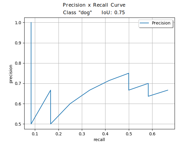
The Precision x Recall curve illustrates the balance between Precision and Recall based on different confidence levels of a detector's bounding boxes. Each point of the plot is computed using a different confidence value.
To demonstrate how to calculate the Average Precision plot, we'll use a practical example from one of the papers mentioned earlier. Consider a dataset of 7 images with 15 ground-truth objects of the same class, as shown in Figure 5. Let's consider that all boxes belong to the same class, "dog" for simplification purposes.
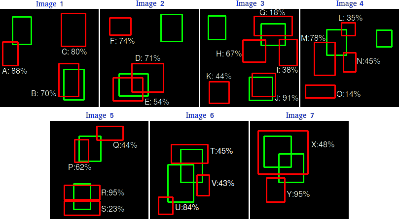
Our hypothetical object detector retrieved 24 objects in our dataset, illustrated by the red boxes. To compute Precision and Recall we use the Precision and Recall equations at all confidence levels to evaluate how well the detector performed for this specific class on our benchmarking dataset. For that, we need to establish some rules:
- Rule 1: For simplicity, let's consider our detections a True Positive (TP) if IOU ≥ 30%; otherwise, it is a False Positive (FP).
- Rule 2: For cases where a detection overlaps with more than one ground-truth (as in Images 2 to 7), the predicted box with the highest IoU is considered TP, and the other is FP.
Based on these rules, we can classify each detection as TP or FP, as shown in Table 1:
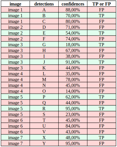
Note that by rule 2, in image 1, "E" is TP while "D" is FP because IoU between "E" and the ground-truth is greater than IoU between "D" and the ground-truth.
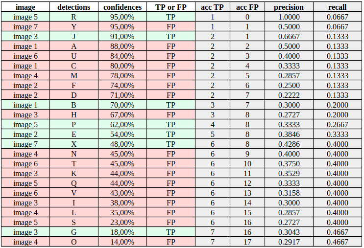
Now, we need to compute Precision and Recall considering the confidence value of each detection. A good way to do so is to sort the detections by their confidence values as shown in Table 2. Then, for each confidence value in each row, we compute the Precision and Recall considering the cumulative TP (acc TP) and cumulative FP (acc FP). The "acc TP" of each row is increased in 1 every time a TP is noted, and the "acc FP" is increased in 1 when a FP is noted. Columns "acc TP" and "acc FP" basically tell us the TP and FP values given a particular confidence level. The computation of each value of Table 2 can be viewed in this spreadsheet.
For example, consider the 12th row (detection "P") of Table 2. The value "acc TP = 4" means that if we benchmark our model on this particular dataset with a confidence of 0.62, we would correctly detect four target objects and incorrectly detect eight target objects. This would result in:
and .
Now, we can plot the Precision x Recall curve with the values, as shown in Figure 6:
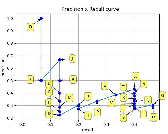
By examining the curve, one may infer the potential trade-offs between Precision and Recall and find a model's optimal operating point based on a selected confidence threshold, even if this threshold is not explicitly depicted on the curve.
If a detector's confidence results in a few false positives (FP), it will likely have high Precision. However, this might lead to missing many true positives (TP), causing a high false negative (FN) rate and, subsequently, low Recall. On the other hand, accepting more positive detections can boost Recall but might also raise the FP count, thereby reducing Precision.
The area under the Precision x Recall curve (AUC) computed for a target class represents the Average Precision value for that particular class. The COCO evaluation approach refers to "AP" as the mean AUC value among all target classes in the image dataset, also referred to as Mean Average Precision (mAP) by other approaches.
For a large dataset, the detector will likely output boxes with a wide range of confidence levels, resulting in a jagged Precision x Recall line, making it challenging to compute its AUC (Average Precision) precisely. Different methods approximate the area of the curve with different approaches. A popular approach is called N-interpolation, where N represents how many points are sampled from the Precision x Recall blue line.
The COCO approach, for instance, uses 101-interpolation, which computes 101 points for equally spaced Recall values (0. , 0.01, 0.02, … 1.00), while other approaches use 11 points (11-interpolation). Figure 7 illustrates a Precision x Recall curve (in blue) with 11 equal-spaced Recall points.
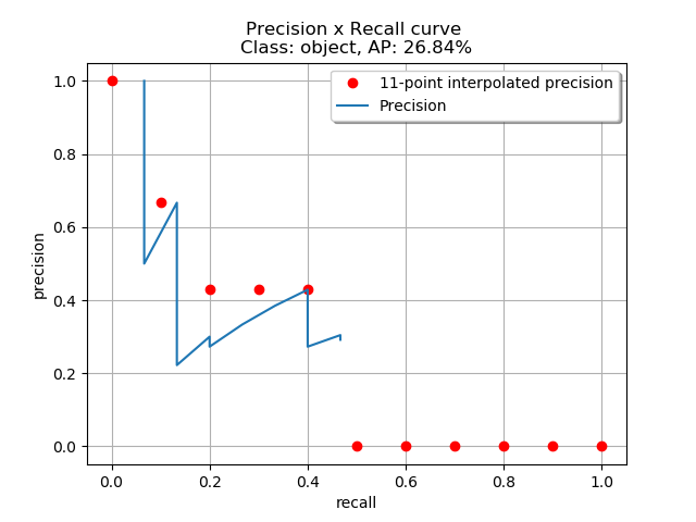
The red points are placed according to the following:
where is the measured Precision at Recall .
In this definition, instead of using the Precision value observed in each Recall level , the Precision is obtained by considering the maximum Precision whose Recall value is greater than .
For this type of approach, the AUC, which represents the Average Precision, is approximated by the average of all points and given by:
What's Average Recall and how to compute it?
Average Recall (AR) is a metric that's often used alongside AP to evaluate object detection models. While AP evaluates both Precision and Recall across different confidence thresholds to provide a single-number summary of model performance, AR focuses solely on the Recall aspect, not taking the confidences into account and considering all detections as positives.
COCO’s approach computes AR as the mean of the maximum obtained Recall over IOUs > 0.5 and classes.
By using IOUs in the range [0.5, 1] and averaging Recall values across this interval, AR assesses the model's predictions on their object localization. Hence, if your goal is to evaluate your model for both high Recall and precise object localization, AR could be a valuable evaluation metric to consider.
What are the variants of Average Precision and Average Recall?
Based on predefined IoU thresholds and the areas associated with ground-truth objects, different versions of AP and AR can be obtained:
- AP@.5: sets IoU threshold = 0.5 and computes the Precision x Recall AUC for each target class in the image dataset. Then, the computed results for each class are summed up and divided by the number of classes.
- AP@.75: uses the same methodology as AP@.50, with IoU threshold = 0.75. With this higher IoU requirement, AP@.75 is considered stricter than AP@.5 and should be used to evaluate models that need to achieve a high level of localization accuracy in their detections.
- AP@[.5:.05:.95]: also referred to AP by cocoeval tools. This is an expanded version of AP@.5 and AP@.75, as it computes AP@ with different IoU thresholds (0.5, 0.55, 0.6,...,0.95) and averages the computed results as shown in the following equation. In comparison to AP@.5 and AP@.75, this metric provides a holistic evaluation, capturing a model’s performance across a broader range of localization accuracies.
- AP-S: It applies AP@[.5:.05:.95] considering (small) ground-truth objects with pixels.
- AP-M: It applies AP@[.5:.05:.95] considering (medium-sized) ground-truth objects with pixels.
- AP-L: It applies AP@[.5:.05:.95] considering (large) ground-truth objects with pixels.
For Average Recall (AR), 10 IoU thresholds (0.5, 0.55, 0.6,...,0.95) are used to compute the Recall values. AR is computed by either limiting the number of detections per image or by limiting the detections based on the object's area.
- AR-1: considers up to 1 detection per image.
- AR-10: considers up to 10 detections per image.
- AR-100: considers up to 100 detections per image.
- AR-S: considers (small) objects with pixels.
- AR-M: considers (medium-sized) objects with pixels.
- AR-L: considers (large) objects with pixels.
Object Detection Leaderboard
We recently released the Object Detection Leaderboard to compare the accuracy and efficiency of open-source models from our Hub.
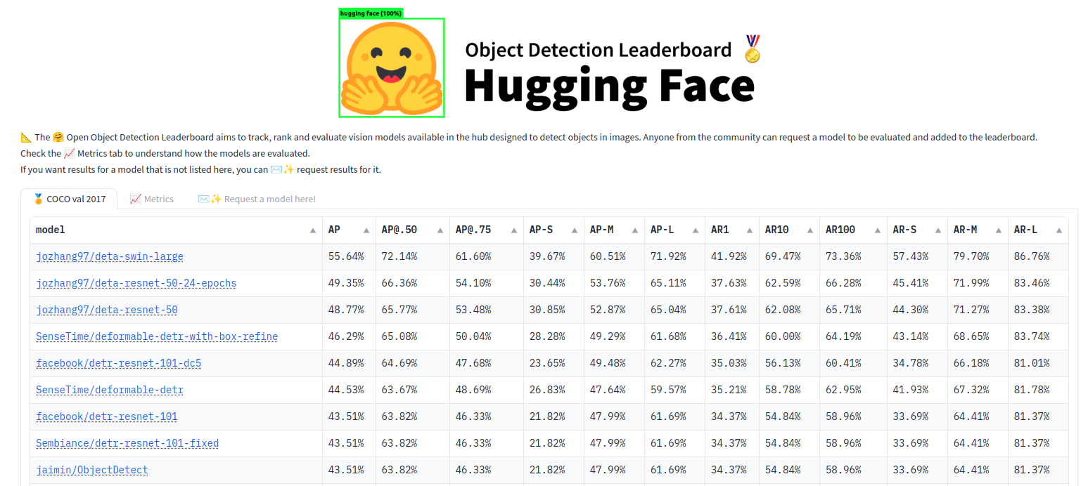
To measure accuracy, we used 12 metrics involving Average Precision and Average Recall using COCO style, benchmarking over COCO val 2017 dataset.
As discussed previously, different tools may adopt different particularities during the evaluation. To prevent results mismatching, we preferred not to implement our version of the metrics. Instead, we opted to use COCO's official evaluation code, also referred to as PyCOCOtools, code available here.
In terms of efficiency, we calculate the frames per second (FPS) for each model using the average evaluation time across the entire dataset, considering pre and post-processing steps. Given the variability in GPU memory requirements for each model, we chose to evaluate with a batch size of 1 (this choice is also influenced by our pre-processing step, which we'll delve into later). However, it's worth noting that this approach may not align perfectly with real-world performance, as larger batch sizes (often containing several images), are commonly used for better efficiency.
Next, we will provide tips on choosing the best model based on the metrics and point out which parameters may interfere with the results. Understanding these nuances is crucial, as this might spark doubts and discussions within the community.
How to pick the best model based on the metrics?
Selecting an appropriate metric to evaluate and compare object detectors considers several factors. The primary considerations include the application's purpose and the dataset's characteristics used to train and evaluate the models.
For general performance, AP (AP@[.5:.05:.95]) is a good choice if you want all-round model performance across different IoU thresholds, without a hard requirement on the localization of the detected objects.
If you want a model with good object recognition and objects generally in the right place, you can look at the AP@.5. If you prefer a more accurate model for placing the bounding boxes, AP@.75 is more appropriate.
If you have restrictions on object sizes, AP-S, AP-M and AP-L come into play. For example, if your dataset or application predominantly features small objects, AP-S provides insights into the detector's efficacy in recognizing such small targets. This becomes crucial in scenarios such as detecting distant vehicles or small artifacts in medical imaging.
Which parameters can impact the Average Precision results?
After picking an object detection model from the Hub, we can vary the output boxes if we use different parameters in the model's pre-processing and post-processing steps. These may influence the assessment metrics. We identified some of the most common factors that may lead to variations in results:
- Ignore detections that have a score under a certain threshold.
- Use
batch_sizes > 1for inference. - Ported models do not output the same logits as the original models.
- Some ground-truth objects may be ignored by the evaluator.
- Computing the IoU may be complicated.
- Text-conditioned models require precise prompts.
Let’s take the DEtection TRansformer (DETR) (facebook/detr-resnet-50) model as our example case. We will show how these factors may affect the output results.
Thresholding detections before evaluation
Our sample model uses the DetrImageProcessor class to process the bounding boxes and logits, as shown in the snippet below:
from transformers import DetrImageProcessor, DetrForObjectDetection
import torch
from PIL import Image
import requests

url = "http://images.cocodataset.org/val2017/000000039769.jpg"
image = Image.open(requests.get(url, stream=True).raw)

processor = DetrImageProcessor.from_pretrained("facebook/detr-resnet-50")
model = DetrForObjectDetection.from_pretrained("facebook/detr-resnet-50")

inputs = processor(images=image, return_tensors="pt")
outputs = model(**inputs)

# PIL images have their size in (w, h) format
target_sizes = torch.tensor([image.size[::-1]])
results = processor.post_process_object_detection(outputs, target_sizes=target_sizes, threshold=0.5)
The parameter threshold in function post_process_object_detection is used to filter the detected bounding boxes based on their confidence scores.
As previously discussed, the Precision x Recall curve is built by measuring the Precision and Recall across the full range of confidence values [0,1]. Thus, limiting the detections before evaluation will produce biased results, as we will leave some detections out.
Varying the batch size
The batch size not only affects the processing time but may also result in different detected boxes. The image pre-processing step may change the resolution of the input images based on their sizes.
As mentioned in DETR documentation, by default, DetrImageProcessor resizes the input images such that the shortest side is 800 pixels, and resizes again so that the longest is at most 1333 pixels. Due to this, images in a batch can have different sizes. DETR solves this by padding images up to the largest size in a batch, and by creating a pixel mask that indicates which pixels are real/which are padding.
To illustrate this process, let's consider the examples in Figure 9 and Figure 10. In Figure 9, we consider batch size = 1, so both images are processed independently with DetrImageProcessor. The first image is resized to (800, 1201), making the detector predict 28 boxes with class vase, 22 boxes with class chair, ten boxes with class bottle, etc.
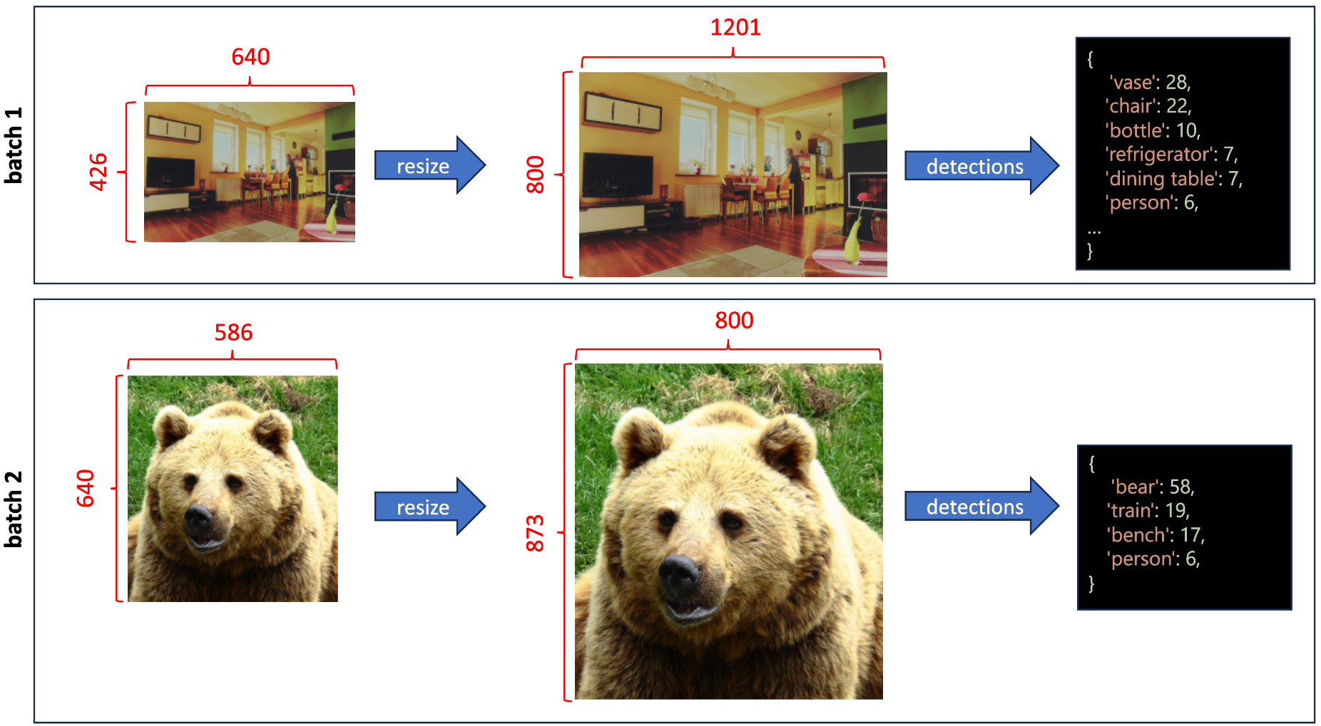
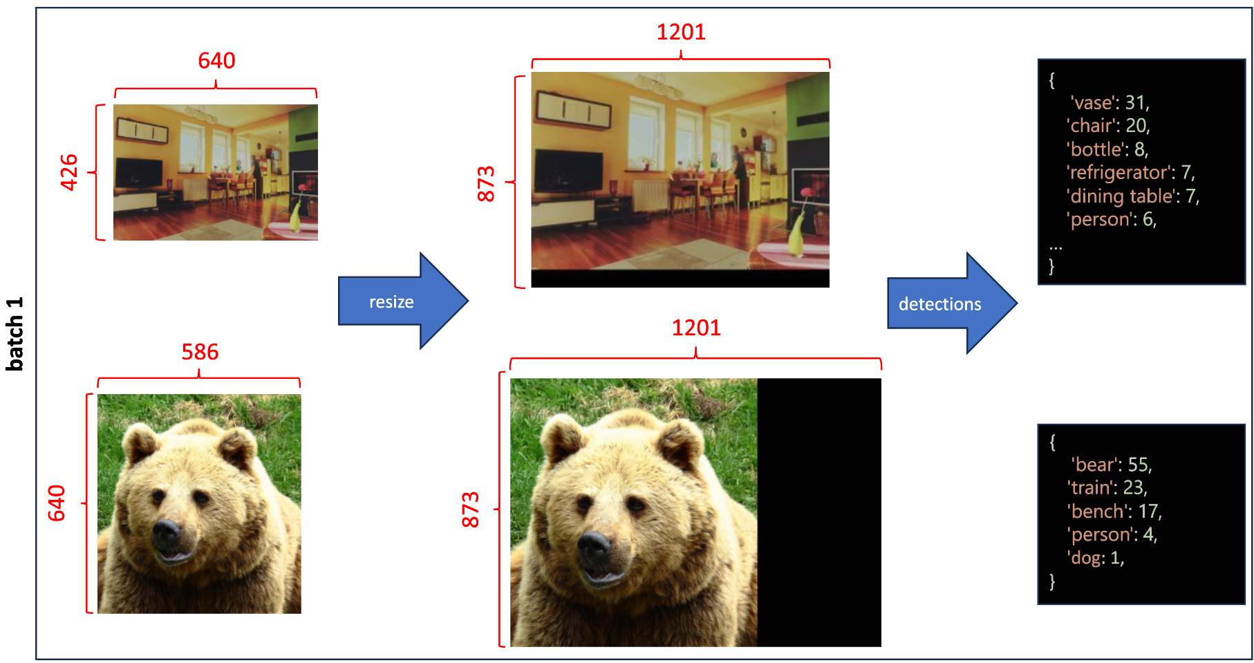
Figure 10 shows the process with batch size = 2, where the same two images are processed with DetrImageProcessor in the same batch. Both images are resized to have the same shape (873, 1201), and padding is applied, so the part of the images with the content is kept with their original aspect ratios. However, the first image, for instance, outputs a different number of objects: 31 boxes with the class vase, 20 boxes with the class chair, eight boxes with the class bottle, etc. Note that for the second image, with batch size = 2, a new class is detected dog. This occurs due to the model's capacity to detect objects of different sizes depending on the image's resolution.
Ported models should output the same logits as the original models
At Hugging Face, we are very careful when porting models to our codebase. Not only with respect to the architecture, clear documentation and coding structure, but we also need to guarantee that the ported models are able to produce the same logits as the original models given the same inputs.
The logits output by a model are post-processed to produce the confidence scores, label IDs, and bounding box coordinates. Thus, minor changes in the logits can influence the metrics results. You may recall the example above, where we discussed the process of computing Average Precision. We showed that confidence levels sort the detections, and small variations may lead to a different order and, thus, different results.
It's important to recognize that models can produce boxes in various formats, and that also may be taken into consideration, making proper conversions required by the evaluator.
- (x, y, width, height): this represents the upper-left corner coordinates followed by the absolute dimensions (width and height).
- (x, y, x2, y2): this format indicates the coordinates of the upper-left corner and the lower-right corner.
- (rel_x_center, rel_y_center, rel_width, rel_height): the values represent the relative coordinates of the center and the relative dimensions of the box.
Some ground-truths are ignored in some benchmarking datasets
Some datasets sometimes use special labels that are ignored during the evaluation process.
COCO, for instance, uses the tag iscrowd to label large groups of objects (e.g. many apples in a basket). During evaluation, objects tagged as iscrowd=1 are ignored. If this is not taken into consideration, you may obtain different results.
Calculating the IoU requires careful consideration
IoU might seem straightforward to calculate based on its definition. However, there's a crucial detail to be aware of: if the ground truth and the detection don't overlap at all, not even by one pixel, the IoU should be 0. To avoid dividing by zero when calculating the union, you can add a small value (called epsilon), to the denominator. However, it's essential to choose epsilon carefully: a value greater than 1e-4 might not be neutral enough to give an accurate result.
Text-conditioned models demand the right prompts
There might be cases in which we want to evaluate text-conditioned models such as OWL-ViT, which can receive a text prompt and provide the location of the desired object.
For such models, different prompts (e.g. "Find the dog" and "Where's the bulldog?") may result in the same results. However, we decided to follow the procedure described in each paper. For the OWL-ViT, for instance, we predict the objects by using the prompt "an image of a {}" where {} is replaced with the benchmarking dataset's classes.
Conclusions
In this post, we introduced the problem of Object Detection and depicted the main metrics used to evaluate them.
As noted, evaluating object detection models may take more work than it looks. The particularities of each model must be carefully taken into consideration to prevent biased results. Also, each metric represents a different point of view of the same model, and picking "the best" metric depends on the model's application and the characteristics of the chosen benchmarking dataset.
Below is a table that illustrates recommended metrics for specific use cases and provides real-world scenarios as examples. However, it's important to note that these are merely suggestions, and the ideal metric can vary based on the distinct particularities of each application.
| Use Case | Real-world Scenarios | Recommended Metric |
|---|---|---|
| General object detection performance | Surveillance, sports analysis | AP |
| Low accuracy requirements (broad detection) | Augmented reality, gesture recognition | AP@.5 |
| High accuracy requirements (tight detection) | Face detection | AP@.75 |
| Detecting small objects | Distant vehicles in autonomous cars, small artifacts in medical imaging | AP-S |
| Medium-sized objects detection | Luggage detection in airport security scans | AP-M |
| Large-sized objects detection | Detecting vehicles in parking lots | AP-L |
| Detecting 1 object per image | Single object tracking in videos | AR-1 |
| Detecting up to 10 objects per image | Pedestrian detection in street cameras | AR-10 |
| Detecting up to 100 objects per image | Crowd counting | AR-100 |
| Recall for small objects | Medical imaging for tiny anomalies | AR-S |
| Recall for medium-sized objects | Sports analysis for players | AR-M |
| Recall for large objects | Wildlife tracking in wide landscapes | AR-L |
The results shown in our 🤗 Object Detection Leaderboard are computed using an independent tool PyCOCOtools widely used by the community for model benchmarking. We're aiming to collect datasets of different domains (e.g. medical images, sports, autonomous vehicles, etc). You can use the discussion page to make requests for datasets, models and features. Eager to see your model or dataset feature on our leaderboard? Don't hold back! Introduce your model and dataset, fine-tune, and let's get it ranked! 🥇
Additional Resources
- Object Detection Guide
- Task of Object Detection
- Paper What Makes for Effective Detection Proposals
- Paper A Comparative Analysis of Object Detection Metrics with a Companion Open-Source Toolkit
- Paper A Survey on Performance Metrics for Object-Detection Algorithms
Special thanks 🙌 to @merve, @osanseviero and @pcuenq for their feedback and great comments. 🤗