makeMoE: Implement a Sparse Mixture of Experts Language Model from Scratch

Community Article Published January 23, 2024

TL;DR: This blog walks through implementing a sparse mixture of experts language model from scratch. This is inspired by and largely based on Andrej Karpathy's project 'makemore' and borrows a number of re-usable components from that implementation. Just like makemore, makeMoE is also an autoregressive character-level language model but uses the aforementioned sparse mixture of experts architecture. The rest of the blog focuses on the key elements of this architecture and how they are implemented. My goal is for you to have an intuitive understanding of how it all works once you read this blog and step through the code in the repo.

The Github repo here provides the end-to-end implementation: https://github.com/AviSoori1x/makeMoE/tree/main

With the release of Mixtral and talk of Llama 3 possibly being a mixture of experts large language model, there is significant interest in this model architecture. However, in sparse mixture of experts language models, much of the components are shared with traditional transformers. Regardless of the seeming simplicity, empirical evidence suggests that training stability is one of the main issues with these models. Hackable small scale implementations such as this may help with rapidly experimenting with new approaches.

In this implementation I make a few significant changes from the makemore architecture:

Sparse mixture of experts instead of the solitary feed forward neural net.
Top-k gating and noisy top-k gating implementations.
initialization - Kaiming He initialization is used here but the point of this notebook is to be hackable so you can swap in Xavier/ Glorot initialization etc. and take it for a spin.

However, the following are unchanged from makemore:

The dataset, preprocessing (tokenization), and the language modeling task Andrej chose originally - generate Shakespeare-like text
Casusal self attention implementation
Training loop
Inference logic

Let's get started!

Sparse mixture of experts language models, as anticipated, depend on self-attention for contextual comprehension. Shortly, we will explore the intricacies of the mixture of experts block. First, let's delve into self-attention to refresh our understanding.

Understanding the intuition of Causal Scaled Dot Product Self Attention

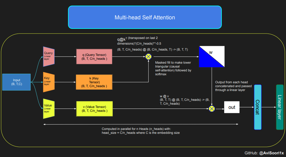
The provided code demonstrates self-attention's mechanics and fundamental concepts, specifically focusing on the classic scaled dot product self-attention. In this variant, the query, key, and value matrices all originate from the same input sequence. To ensure the integrity of the autoregressive language generation process, particularly in a decoder-only model, the code implements masking. This masking technique is crucial as it obscures any information following the current token's position, thereby directing the model's attention to only the preceding parts of the sequence. Such an attention mechanism is known as causal self-attention. It's important to note that the Sparse Mixture of Experts model isn't restricted to decoder-only Transformer architectures. In fact, much of the significant work in this field, particularly that by Shazeer et al, revolves around the T5 architecture, which encompasses both encoder and decoder components in the Transformer model.

#This code is borrowed from Andrej Karpathy's makemore repository linked in the repo.
The self attention layers in Sparse mixture of experts models are the same as
in regular transformer models

torch.manual_seed(1337)
B,T,C = 4,8,32 # batch, time, channels
x = torch.randn(B,T,C)

# let's see a single Head perform self-attention
head_size = 16
key = nn.Linear(C, head_size, bias=False)
query = nn.Linear(C, head_size, bias=False)
value = nn.Linear(C, head_size, bias=False)
k = key(x)   # (B, T, 16)
q = query(x) # (B, T, 16)
wei =  q @ k.transpose(-2, -1) # (B, T, 16) @ (B, 16, T) ---> (B, T, T)

tril = torch.tril(torch.ones(T, T))
#wei = torch.zeros((T,T))
wei = wei.masked_fill(tril == 0, float('-inf'))
wei = F.softmax(wei, dim=-1) #B,T,T

v = value(x) #B,T,H
out = wei @ v # (B,T,T) @ (B,T,H) -> (B,T,H)
out.shape

torch.Size([4, 8, 16])

The code for causal self attention and multi-head causal self attention can be organized as follows. Multi-head self attention applies multiple attention heads in parallel, each focusing on a separate section of the channel (the embedding dimension). Multi-head self attention essentially improves the learning process and improves efficiency of model training due to the inherently parallel implementation. Notice I have used dropout throughout this implementation for regularization i.e. preventing overfitting.

#Causal scaled dot product self-Attention Head
n_embd = 64
n_head = 4
n_layer = 4
head_size = 16
dropout = 0.1

class Head(nn.Module):
    """ one head of self-attention """

    def __init__(self, head_size):
        super().__init__()
        self.key = nn.Linear(n_embd, head_size, bias=False)
        self.query = nn.Linear(n_embd, head_size, bias=False)
        self.value = nn.Linear(n_embd, head_size, bias=False)
        self.register_buffer('tril', torch.tril(torch.ones(block_size, block_size)))

        self.dropout = nn.Dropout(dropout)

    def forward(self, x):
        B,T,C = x.shape
        k = self.key(x)   # (B,T,C)
        q = self.query(x) # (B,T,C)
        # compute attention scores ("affinities")
        wei = q @ k.transpose(-2,-1) * C**-0.5 # (B, T, C) @ (B, C, T) -> (B, T, T)
        wei = wei.masked_fill(self.tril[:T, :T] == 0, float('-inf')) # (B, T, T)
        wei = F.softmax(wei, dim=-1) # (B, T, T)
        wei = self.dropout(wei)
        # perform the weighted aggregation of the values
        v = self.value(x) # (B,T,C)
        out = wei @ v # (B, T, T) @ (B, T, C) -> (B, T, C)
        return out

Multi-head self attention is implemented as follows:

#Multi-Headed Self Attention
class MultiHeadAttention(nn.Module):
    """ multiple heads of self-attention in parallel """

    def __init__(self, num_heads, head_size):
        super().__init__()
        self.heads = nn.ModuleList([Head(head_size) for _ in range(num_heads)])
        self.proj = nn.Linear(n_embd, n_embd)
        self.dropout = nn.Dropout(dropout)

    def forward(self, x):
        out = torch.cat([h(x) for h in self.heads], dim=-1)
        out = self.dropout(self.proj(out))
        return out

Creating an Expert module i.e. a simple Multi Layer Perceptron

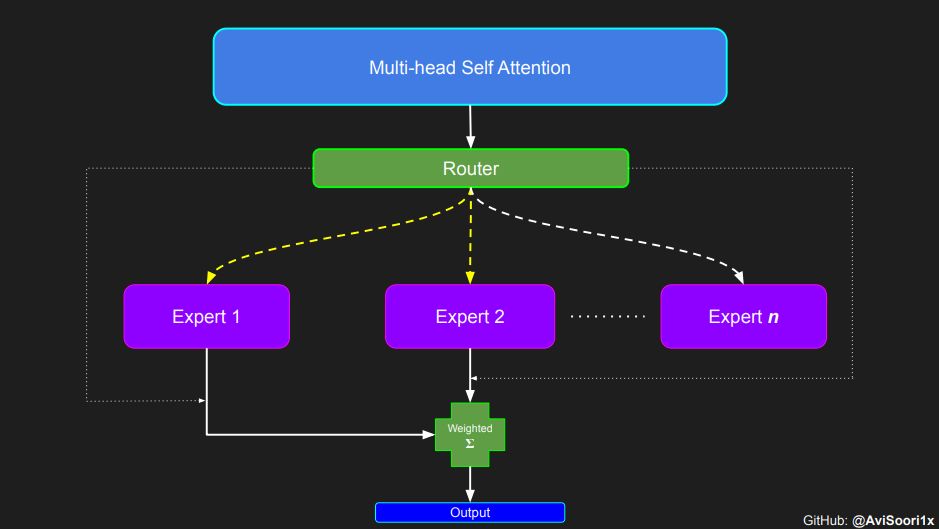
In the Sparse Mixture of Experts (MoE) architecture, the self-attention mechanism within each transformer block remains unchanged. However, a notable alteration occurs in the structure of each block: the standard feed-forward neural network is replaced with several sparsely activated feed-forward networks, known as experts. "Sparse activation" refers to the process where each token in the sequence is routed to only a limited number of these experts – typically one or two – out of the total pool available. This helps with training and inference speed, as a handful of experts are activated in each forward pass. However, all the experts have to be in GPU memory, thus creating interesting deployments issues when the total parameter count reaches hundreds of billions or even trillions.

#Expert module
class Expert(nn.Module):
    """ An MLP is a simple linear layer followed by a non-linearity i.e. each Expert """

    def __init__(self, n_embd):
        super().__init__()
        self.net = nn.Sequential(
            nn.Linear(n_embd, 4 * n_embd),
            nn.ReLU(),
            nn.Linear(4 * n_embd, n_embd),
            nn.Dropout(dropout),
        )

    def forward(self, x):
        return self.net(x)

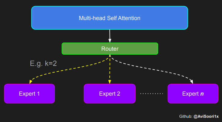
Top-k Gating Intuition through an Example

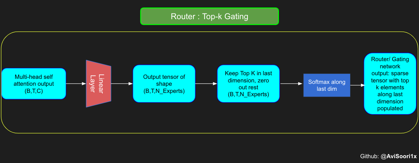
The gating network, also known as the router, determines which expert network receives the output for each token from the multi-head attention. Let's consider a simple example: suppose there are 4 experts, and the token is to be routed to the top 2 experts. Initially, we input the token into the gating network through a linear layer. This layer projects the input tensor from a shape of (2, 4, 32) — representing (Batch size, Tokens, n_embed, where n_embed is the channel dimension of the input) — to a new shape of (2, 4, 4), which corresponds to (Batch size, Tokens, num_experts), where num_experts is the count of expert networks. Following this, we determine the top k=2 highest values and their respective indices along the last dimension.

#Understanding how gating works
num_experts = 4
top_k=2
n_embed=32


#Example multi-head attention output for a simple illustrative example, consider n_embed=32, context_length=4 and batch_size=2
mh_output = torch.randn(2, 4, n_embed)

topkgate_linear = nn.Linear(n_embed, num_experts) # nn.Linear(32, 4)

logits = topkgate_linear(mh_output)
top_k_logits, top_k_indices = logits.topk(top_k, dim=-1)  # Get top-k experts
top_k_logits, top_k_indices

#output:
(tensor([[[ 0.0246, -0.0190],
          [ 0.1991,  0.1513],
          [ 0.9749,  0.7185],
          [ 0.4406, -0.8357]],
 
         [[ 0.6206, -0.0503],
          [ 0.8635,  0.3784],
          [ 0.6828,  0.5972],
          [ 0.4743,  0.3420]]], grad_fn=<TopkBackward0>),
 tensor([[[2, 3],
          [2, 1],
          [3, 1],
          [2, 1]],
 
         [[0, 2],
          [0, 3],
          [3, 2],
          [3, 0]]]))

Obtain the sparse gating output by only keeping the top k values in their respective index along the last dimension. Fill the rest with '-inf' and pass through a softmax activation. This pushes '-inf' values to zero, makes the top two values more accentuated and sum to 1. This summation to 1 helps with the weighting of expert outputs

zeros = torch.full_like(logits, float('-inf')) #full_like clones a tensor and fills it with a specified value (like infinity) for masking or calculations.
sparse_logits = zeros.scatter(-1, top_k_indices, top_k_logits)
sparse_logits

#output
tensor([[[   -inf,    -inf,  0.0246, -0.0190],
         [   -inf,  0.1513,  0.1991,    -inf],
         [   -inf,  0.7185,    -inf,  0.9749],
         [   -inf, -0.8357,  0.4406,    -inf]],

        [[ 0.6206,    -inf, -0.0503,    -inf],
         [ 0.8635,    -inf,    -inf,  0.3784],
         [   -inf,    -inf,  0.5972,  0.6828],
         [ 0.3420,    -inf,    -inf,  0.4743]]], grad_fn=<ScatterBackward0>)

gating_output= F.softmax(sparse_logits, dim=-1)
gating_output

#ouput
tensor([[[0.0000, 0.0000, 0.5109, 0.4891],
         [0.0000, 0.4881, 0.5119, 0.0000],
         [0.0000, 0.4362, 0.0000, 0.5638],
         [0.0000, 0.2182, 0.7818, 0.0000]],

        [[0.6617, 0.0000, 0.3383, 0.0000],
         [0.6190, 0.0000, 0.0000, 0.3810],
         [0.0000, 0.0000, 0.4786, 0.5214],
         [0.4670, 0.0000, 0.0000, 0.5330]]], grad_fn=<SoftmaxBackward0>)

Generalizing and Modularizing above code and adding noisy top-k Gating for load balancing

# First define the top k router module 
class TopkRouter(nn.Module):
    def __init__(self, n_embed, num_experts, top_k):
        super(TopkRouter, self).__init__()
        self.top_k = top_k
        self.linear =nn.Linear(n_embed, num_experts)
    
    def forward(self, mh_ouput):
        # mh_ouput is the output tensor from multihead self attention block
        logits = self.linear(mh_output)
        top_k_logits, indices = logits.topk(self.top_k, dim=-1)
        zeros = torch.full_like(logits, float('-inf'))
        sparse_logits = zeros.scatter(-1, indices, top_k_logits)
        router_output = F.softmax(sparse_logits, dim=-1)
        return router_output, indices

Let's test the functionality with some sample inputs:

#Testing this out:
num_experts = 4
top_k = 2
n_embd = 32

mh_output = torch.randn(2, 4, n_embd)  # Example input
top_k_gate = TopkRouter(n_embd, num_experts, top_k)
gating_output, indices = top_k_gate(mh_output)
gating_output.shape, gating_output, indices
#And it works!!

#output
(torch.Size([2, 4, 4]),
 tensor([[[0.5284, 0.0000, 0.4716, 0.0000],
          [0.0000, 0.4592, 0.0000, 0.5408],
          [0.0000, 0.3529, 0.0000, 0.6471],
          [0.3948, 0.0000, 0.0000, 0.6052]],
 
         [[0.0000, 0.5950, 0.4050, 0.0000],
          [0.4456, 0.0000, 0.5544, 0.0000],
          [0.7208, 0.0000, 0.0000, 0.2792],
          [0.0000, 0.0000, 0.5659, 0.4341]]], grad_fn=<SoftmaxBackward0>),
 tensor([[[0, 2],
          [3, 1],
          [3, 1],
          [3, 0]],
 
         [[1, 2],
          [2, 0],
          [0, 3],
          [2, 3]]]))

Althought the mixtral paper released recently does not make any mention of it, I believe Noisy top-k Gating is an important tool in training MoE models. Essentially, you don't want all the tokens to be sent to the same set of 'favored' experts. You want a fine balance of exploitation and exploration. For this purpose, to load balance, it is helpful to add standard normal noise to the logits from the gating linear layer. This makes training more efficient

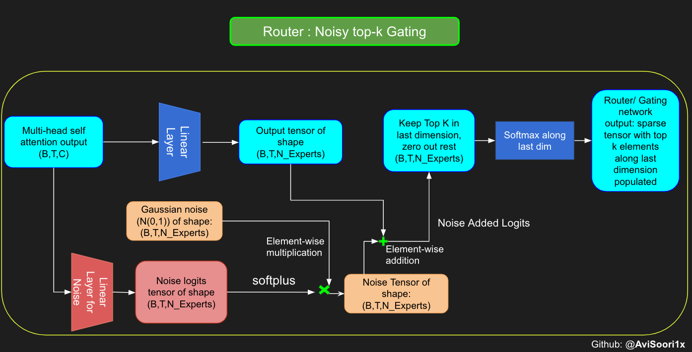
#Changing the above to accomodate noisy top-k gating
class NoisyTopkRouter(nn.Module):
    def __init__(self, n_embed, num_experts, top_k):
        super(NoisyTopkRouter, self).__init__()
        self.top_k = top_k
        #layer for router logits
        self.topkroute_linear = nn.Linear(n_embed, num_experts)
        self.noise_linear =nn.Linear(n_embed, num_experts)

    
    def forward(self, mh_output):
        # mh_ouput is the output tensor from multihead self attention block
        logits = self.topkroute_linear(mh_output)

        #Noise logits
        noise_logits = self.noise_linear(mh_output)

        #Adding scaled unit gaussian noise to the logits
        noise = torch.randn_like(logits)*F.softplus(noise_logits)
        noisy_logits = logits + noise

        top_k_logits, indices = noisy_logits.topk(self.top_k, dim=-1)
        zeros = torch.full_like(noisy_logits, float('-inf'))
        sparse_logits = zeros.scatter(-1, indices, top_k_logits)
        router_output = F.softmax(sparse_logits, dim=-1)
        return router_output, indices

Let's test this implementation out again

#Testing this out, again:
num_experts = 8
top_k = 2
n_embd = 16

mh_output = torch.randn(2, 4, n_embd)  # Example input
noisy_top_k_gate = NoisyTopkRouter(n_embd, num_experts, top_k)
gating_output, indices = noisy_top_k_gate(mh_output)
gating_output.shape, gating_output, indices
#It works!!

#output
(torch.Size([2, 4, 8]),
 tensor([[[0.4181, 0.0000, 0.5819, 0.0000, 0.0000, 0.0000, 0.0000, 0.0000],
          [0.4693, 0.5307, 0.0000, 0.0000, 0.0000, 0.0000, 0.0000, 0.0000],
          [0.0000, 0.4985, 0.5015, 0.0000, 0.0000, 0.0000, 0.0000, 0.0000],
          [0.0000, 0.0000, 0.0000, 0.2641, 0.0000, 0.7359, 0.0000, 0.0000]],
 
         [[0.0000, 0.0000, 0.0000, 0.6301, 0.0000, 0.3699, 0.0000, 0.0000],
          [0.0000, 0.0000, 0.0000, 0.4766, 0.0000, 0.0000, 0.0000, 0.5234],
          [0.0000, 0.0000, 0.0000, 0.6815, 0.0000, 0.0000, 0.3185, 0.0000],
          [0.4482, 0.5518, 0.0000, 0.0000, 0.0000, 0.0000, 0.0000, 0.0000]]],
        grad_fn=<SoftmaxBackward0>),
 tensor([[[2, 0],
          [1, 0],
          [2, 1],
          [5, 3]],
 
         [[3, 5],
          [7, 3],
          [3, 6],
          [1, 0]]]))

Creating a sparse Mixture of Experts module

The primary aspect of this process involves the gating network's output. After acquiring these results, the top k values are selectively multiplied with the outputs from the corresponding top-k experts for a given token. This selective multiplication forms a weighted sum, which constitutes the SparseMoe block's output. The critical and challenging part of this process is to avoid unnecessary multiplications. It's essential to conduct forward passes only for the top_k experts and then compute this weighted sum. Performing forward passes for each expert would defeat the purpose of employing a sparse MoE, as it would no longer be sparse.

class SparseMoE(nn.Module):
    def __init__(self, n_embed, num_experts, top_k):
        super(SparseMoE, self).__init__()
        self.router = NoisyTopkRouter(n_embed, num_experts, top_k)
        self.experts = nn.ModuleList([Expert(n_embed) for _ in range(num_experts)])
        self.top_k = top_k

    def forward(self, x):
        gating_output, indices = self.router(x)
        final_output = torch.zeros_like(x)

        # Reshape inputs for batch processing
        flat_x = x.view(-1, x.size(-1))
        flat_gating_output = gating_output.view(-1, gating_output.size(-1))

        # Process each expert in parallel
        for i, expert in enumerate(self.experts):
            # Create a mask for the inputs where the current expert is in top-k
            expert_mask = (indices == i).any(dim=-1)
            flat_mask = expert_mask.view(-1)

            if flat_mask.any():
                expert_input = flat_x[flat_mask]
                expert_output = expert(expert_input)

                # Extract and apply gating scores
                gating_scores = flat_gating_output[flat_mask, i].unsqueeze(1)
                weighted_output = expert_output * gating_scores

                # Update final output additively by indexing and adding
                final_output[expert_mask] += weighted_output.squeeze(1)

        return final_output

It is helpful to test with sample inputs whether the above implementation works or not. Upon running the following code we can see it does!

import torch
import torch.nn as nn

#Let's test this out
num_experts = 8
top_k = 2
n_embd = 16
dropout=0.1

mh_output = torch.randn(4, 8, n_embd)  # Example multi-head attention output
sparse_moe = SparseMoE(n_embd, num_experts, top_k)
final_output = sparse_moe(mh_output)
print("Shape of the final output:", final_output.shape)

Shape of the final output: torch.Size([4, 8, 16])

To emphasize, it's important to recognize that the magnitudes of the top_k experts output from the Router/ gating network, as illustrated in the code above, are also significant. These top_k indices identify the experts that are activated, and the magnitude of the values in those top_k dimensions determines their respective weighting. This concept of weighted summation is further highlighted in the diagram below.

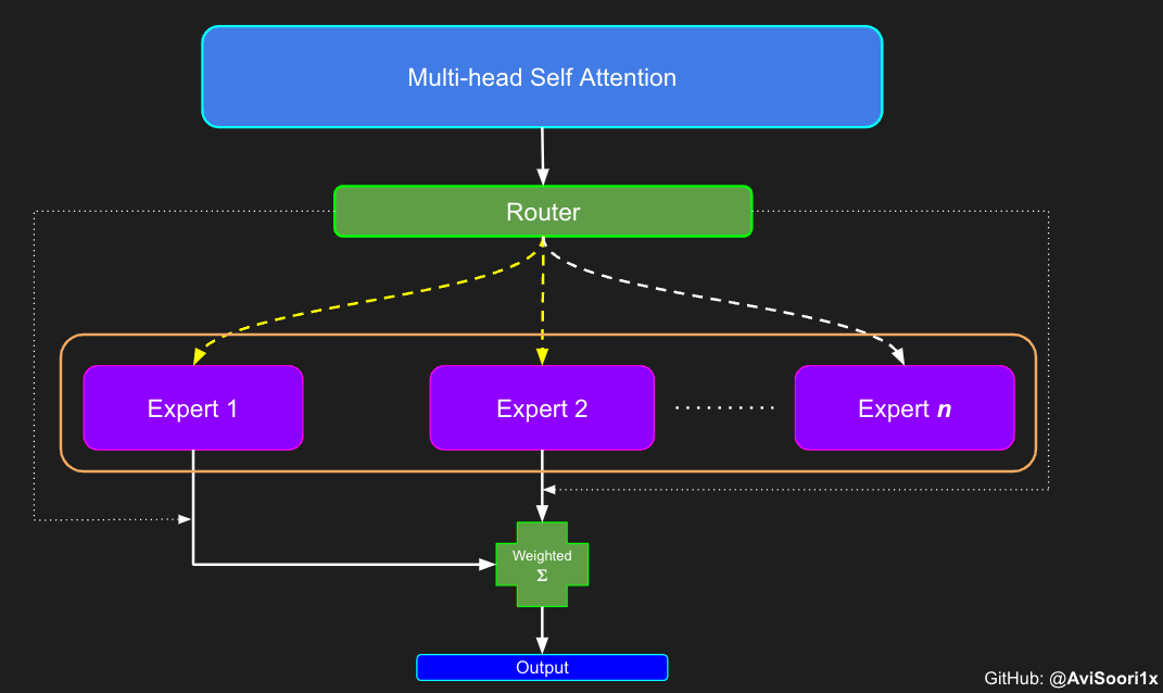
Putting it all together

Multi-head self attention and sparse mixture of experts are combined to form a sparse mixture of experts transformer block. Just like in a vanilla transformer block, skip connections are added to ensure the training is stable and issues like vanishing gradient are avoided. Also, layer normalization is employed to further stabilize the learning process.

#Create a self attention + mixture of experts block, that may be repeated several number of times 
class Block(nn.Module):
    """ Mixture of Experts Transformer block: communication followed by computation (multi-head self attention + SparseMoE) """

    def __init__(self, n_embed, n_head, num_experts, top_k):
        # n_embed: embedding dimension, n_head: the number of heads we'd like
        super().__init__()
        head_size = n_embed // n_head
        self.sa = MultiHeadAttention(n_head, head_size)
        self.smoe = SparseMoE(n_embed, num_experts, top_k)
        self.ln1 = nn.LayerNorm(n_embed)
        self.ln2 = nn.LayerNorm(n_embed)

    def forward(self, x):
        x = x + self.sa(self.ln1(x))
        x = x + self.smoe(self.ln2(x))
        return x

Finally putting it all together to crease a sparse mixture of experts language model

class SparseMoELanguageModel(nn.Module):

    def __init__(self):
        super().__init__()
        # each token directly reads off the logits for the next token from a lookup table
        self.token_embedding_table = nn.Embedding(vocab_size, n_embed)
        self.position_embedding_table = nn.Embedding(block_size, n_embed)
        self.blocks = nn.Sequential(*[Block(n_embed, n_head=n_head, num_experts=num_experts,top_k=top_k) for _ in range(n_layer)])
        self.ln_f = nn.LayerNorm(n_embed) # final layer norm
        self.lm_head = nn.Linear(n_embed, vocab_size)

    def forward(self, idx, targets=None):
        B, T = idx.shape

        # idx and targets are both (B,T) tensor of integers
        tok_emb = self.token_embedding_table(idx) # (B,T,C)
        pos_emb = self.position_embedding_table(torch.arange(T, device=device)) # (T,C)
        x = tok_emb + pos_emb # (B,T,C)
        x = self.blocks(x) # (B,T,C)
        x = self.ln_f(x) # (B,T,C)
        logits = self.lm_head(x) # (B,T,vocab_size)

        if targets is None:
            loss = None
        else:
            B, T, C = logits.shape
            logits = logits.view(B*T, C)
            targets = targets.view(B*T)
            loss = F.cross_entropy(logits, targets)

        return logits, loss

    def generate(self, idx, max_new_tokens):
        # idx is (B, T) array of indices in the current context
        for _ in range(max_new_tokens):
            # crop idx to the last block_size tokens
            idx_cond = idx[:, -block_size:]
            # get the predictions
            logits, loss = self(idx_cond)
            # focus only on the last time step
            logits = logits[:, -1, :] # becomes (B, C)
            # apply softmax to get probabilities
            probs = F.softmax(logits, dim=-1) # (B, C)
            # sample from the distribution
            idx_next = torch.multinomial(probs, num_samples=1) # (B, 1)
            # append sampled index to the running sequence
            idx = torch.cat((idx, idx_next), dim=1) # (B, T+1)
        return idx

Initialization is important for efficient training of deep neural nets. Kaiming He initialization is used here because of presence of ReLU activations in the experts. Feel free to experiment with Glorot initialization which is more commonly used in transformers. Jeremy Howard's Fastai Part 2 has an excellent lecture that implements these from scratch: https://course.fast.ai/Lessons/lesson17.html. It is noted in literature that Glorot initialization is commonly used in transformer models, so this is an opportunity to possibly improve model performance.

def kaiming_init_weights(m):
    if isinstance (m, (nn.Linear)): 
        init.kaiming_normal_(m.weight)

model = SparseMoELanguageModel()
model.apply(kaiming_init_weights)

I have used mlflow to track and log important metrics and the training hyperparameters. The training loop I've shown here includes this code. If you prefer to just train without using mlflow, the notebooks in the makeMoE github repo have code blocks without MLFlow. I personally find it very convenient to track parameters and metrics, particularly when experimenting.

#Using MLFlow
m = model.to(device)
# print the number of parameters in the model
print(sum(p.numel() for p in m.parameters())/1e6, 'M parameters')

# create a PyTorch optimizer
optimizer = torch.optim.AdamW(model.parameters(), lr=learning_rate)
#mlflow.set_experiment("makeMoE")
with mlflow.start_run():
    #If you use mlflow.autolog() this will be automatically logged. I chose to explicitly log here for completeness
    params = {"batch_size": batch_size , "block_size" : block_size, "max_iters": max_iters, "eval_interval": eval_interval,
              "learning_rate": learning_rate, "device": device, "eval_iters": eval_iters, "dropout" : dropout, "num_experts": num_experts, "top_k": top_k }
    mlflow.log_params(params)
    for iter in range(max_iters):

        # every once in a while evaluate the loss on train and val sets
        if iter % eval_interval == 0 or iter == max_iters - 1:
            losses = estimate_loss()
            print(f"step {iter}: train loss {losses['train']:.4f}, val loss {losses['val']:.4f}")
            metrics = {"train_loss": losses['train'], "val_loss": losses['val']}
            mlflow.log_metrics(metrics, step=iter)


        # sample a batch of data
        xb, yb = get_batch('train')

        # evaluate the loss
        logits, loss = model(xb, yb)
        optimizer.zero_grad(set_to_none=True)
        loss.backward()
        optimizer.step()

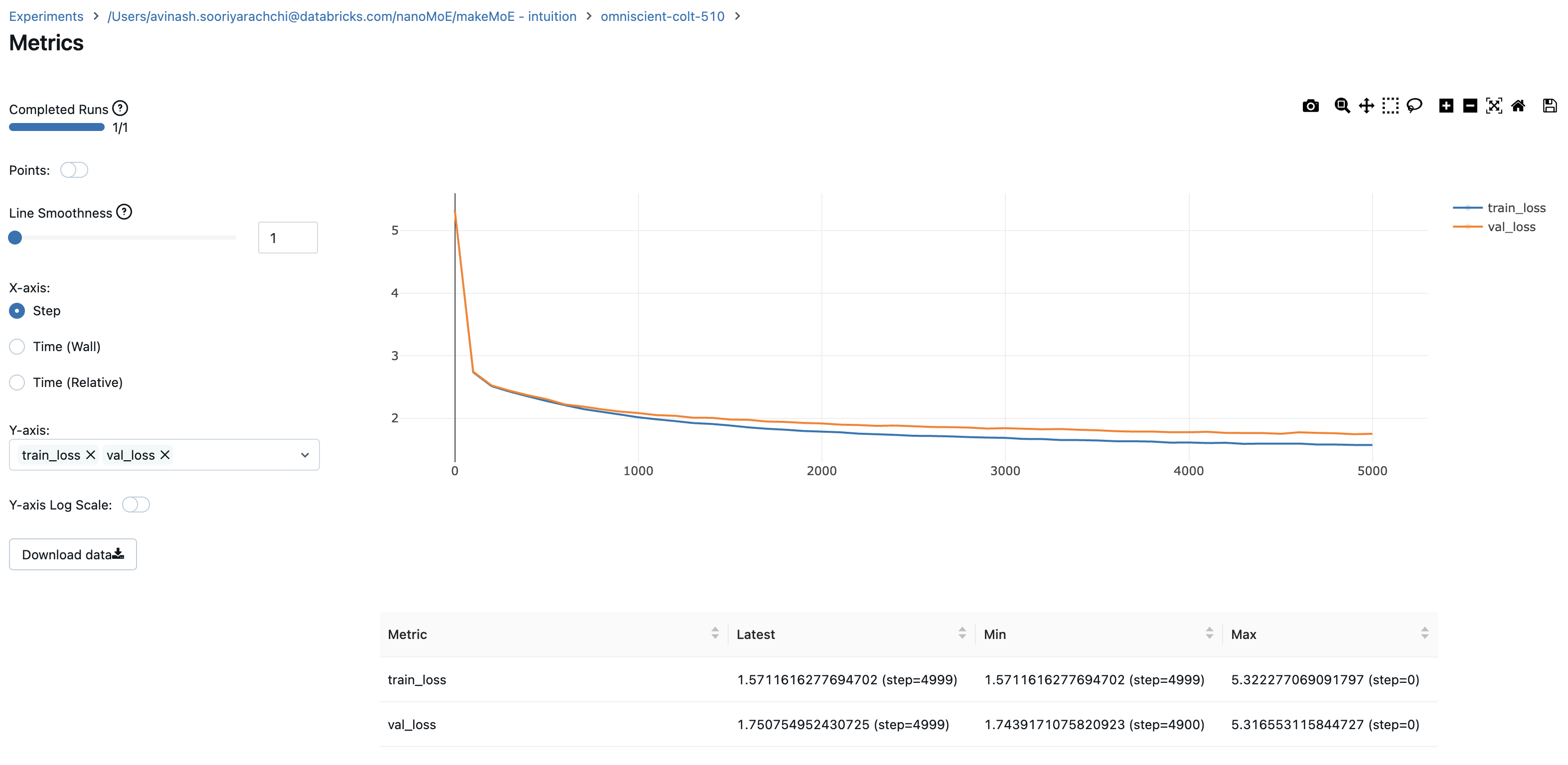
8.996545 M parameters
step 0: train loss 5.3223, val loss 5.3166
step 100: train loss 2.7351, val loss 2.7429
step 200: train loss 2.5125, val loss 2.5233
.
.
.

step 4999: train loss 1.5712, val loss 1.7508

Logging train and validation losses gives you a good indication of how the training is going. The plot shows that I probably should have stopped around 4500 steps (when the validation loss slightly jumps up)

Now we can generate text using this model character by character, autoregressively. For a sparsely activated ~9M parameter model, I can't complain.

# generate from the model. Not great. Not too bad either
context = torch.zeros((1, 1), dtype=torch.long, device=device)
print(decode(m.generate(context, max_new_tokens=2000)[0].tolist()))

DUKE VINCENVENTIO:
If it ever fecond he town sue kigh now,
That thou wold'st is steen 't.

SIMNA:
Angent her; no, my a born Yorthort,
Romeoos soun and lawf to your sawe with ch a woft ttastly defy,
To declay the soul art; and meart smad.

CORPIOLLANUS:
Which I cannot shall do from by born und ot cold warrike,
What king we best anone wrave's going of heard and good
Thus playvage; you have wold the grace.
...

I hope this explanation has helped to build your understanding of the Sparse Mixture of Experts model architecture and how it comes together.

I referenced the following publications heavily for this implementation:

Mixtral of experts: https://arxiv.org/pdf/2401.04088.pdf
Outrageously Large Neural Networks: The Sparsely-Gated Mixture-Of-Experts layer: https://arxiv.org/pdf/1701.06538.pdf

Original makemore implementation from Andrej Karpathy:

https://github.com/karpathy/makemore

The code was entirely developed on Databricks using a single A100. If you're running this on Databricks, you can scale this on an arbitrarily large GPU cluster with no issues,on the cloud provider of your choice. I chose to use MLFlow (which comes pre-installed in Databricks. It is fully open source and you can pip install easily elsewhere) as I find it helpful to track and log all the metrics necessary. This is entirely optional. Please note that the implementation emphasizes readability and hackability vs. performance, so there are many ways in which you could improve this.

Given that, here are few things that you could try:

Make the Mixture of Experts module more efficient. I believe significant improvements could be made in the above implementation for the sparse activation of the correct experts.
Try different neural net initialization strategies. The source I've listed (Fastai part 2) is excellent
Go from character level to sub-word tokenization
Do Bayesian hyperparaeter search for the number of experts and top_k (the number of experts activated for each token). This could losely be categorized as neural architecture search.
Expert Capacity is not discussed or implemented here. It is definitely worth exploring.

With the amount of interest in mixture of experts and multimodality, it will also be interesting to see what is going to be devloped at the intersection of the two. Happy hacking!!

PS: Part 2 of this blog with the implementation of Expert Capacity for more efficient training is given here: https://huggingface.co/blog/AviSoori1x/makemoe2

Upvote