Deep RL Course documentation
Visualize the Clipped Surrogate Objective Function
Visualize the Clipped Surrogate Objective Function
Don’t worry. It’s normal if this seems complex to handle right now. But we’re going to see what this Clipped Surrogate Objective Function looks like, and this will help you to visualize better what’s going on.
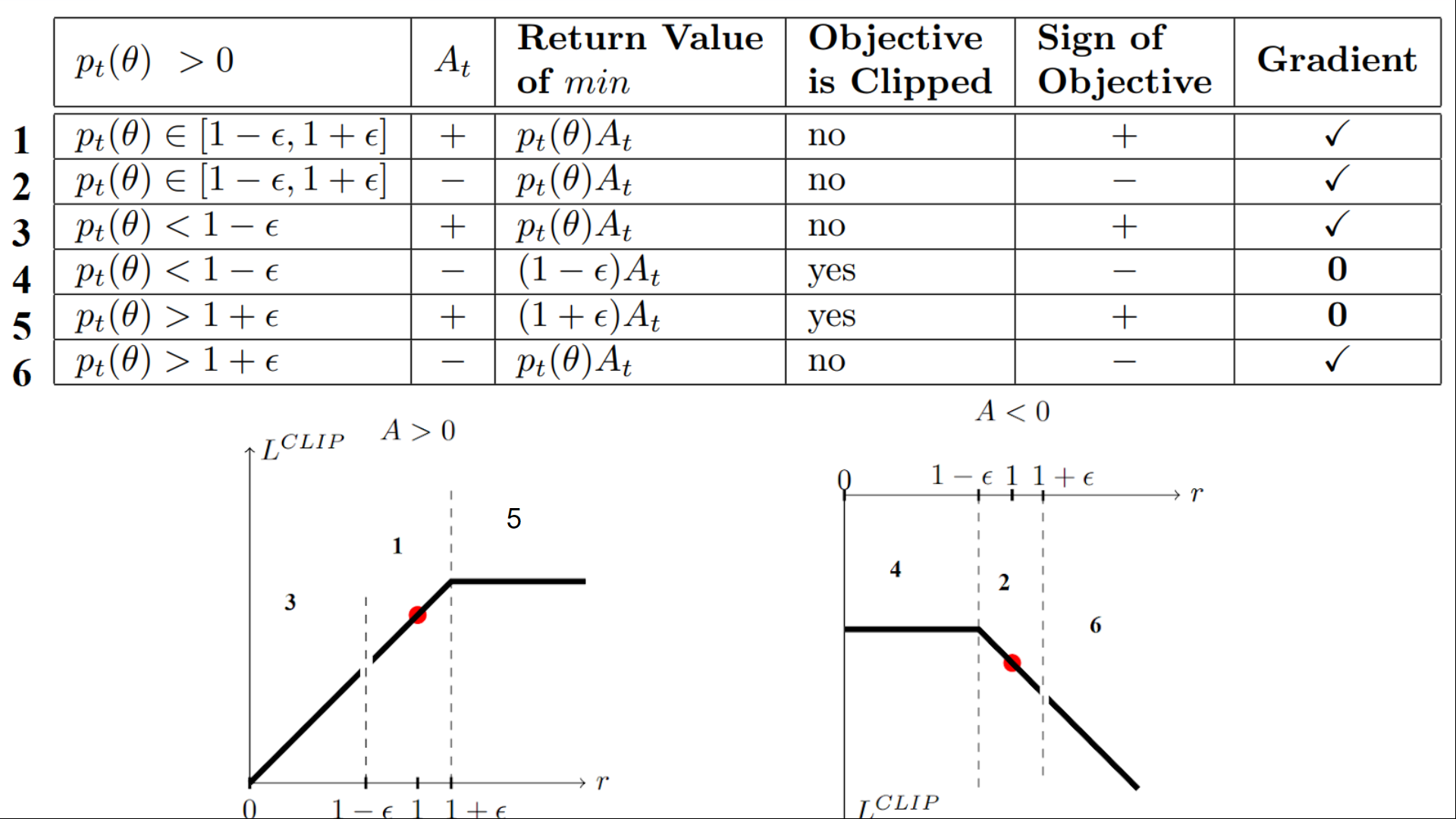
We have six different situations. Remember first that we take the minimum between the clipped and unclipped objectives.
Case 1 and 2: the ratio is between the range
In situations 1 and 2, the clipping does not apply since the ratio is between the range
In situation 1, we have a positive advantage: the action is better than the average of all the actions in that state. Therefore, we should encourage our current policy to increase the probability of taking that action in that state.
Since the ratio is between intervals, we can increase our policy’s probability of taking that action at that state.
In situation 2, we have a negative advantage: the action is worse than the average of all actions at that state. Therefore, we should discourage our current policy from taking that action in that state.
Since the ratio is between intervals, we can decrease the probability that our policy takes that action at that state.
Case 3 and 4: the ratio is below the range
If the probability ratio is lower than, the probability of taking that action at that state is much lower than with the old policy.
If, like in situation 3, the advantage estimate is positive (A>0), then you want to increase the probability of taking that action at that state.
But if, like situation 4, the advantage estimate is negative, we don’t want to decrease further the probability of taking that action at that state. Therefore, the gradient is = 0 (since we’re on a flat line), so we don’t update our weights.
Case 5 and 6: the ratio is above the range
If the probability ratio is higher than, the probability of taking that action at that state in the current policy is much higher than in the former policy.
If, like in situation 5, the advantage is positive, we don’t want to get too greedy. We already have a higher probability of taking that action at that state than the former policy. Therefore, the gradient is = 0 (since we’re on a flat line), so we don’t update our weights.
If, like in situation 6, the advantage is negative, we want to decrease the probability of taking that action at that state.
So if we recap, we only update the policy with the unclipped objective part. When the minimum is the clipped objective part, we don’t update our policy weights since the gradient will equal 0.
So we update our policy only if:
- Our ratio is in the range
- Our ratio is outside the range, but the advantage leads to getting closer to the range
- Being below the ratio but the advantage is > 0
- Being above the ratio but the advantage is < 0
You might wonder why, when the minimum is the clipped ratio, the gradient is 0. When the ratio is clipped, the derivative in this case will not be the derivative of the but the derivative of either or the derivative of which both = 0.
To summarize, thanks to this clipped surrogate objective, we restrict the range that the current policy can vary from the old one. Because we remove the incentive for the probability ratio to move outside of the interval since the clip forces the gradient to be zero. If the ratio is > or < the gradient will be equal to 0.
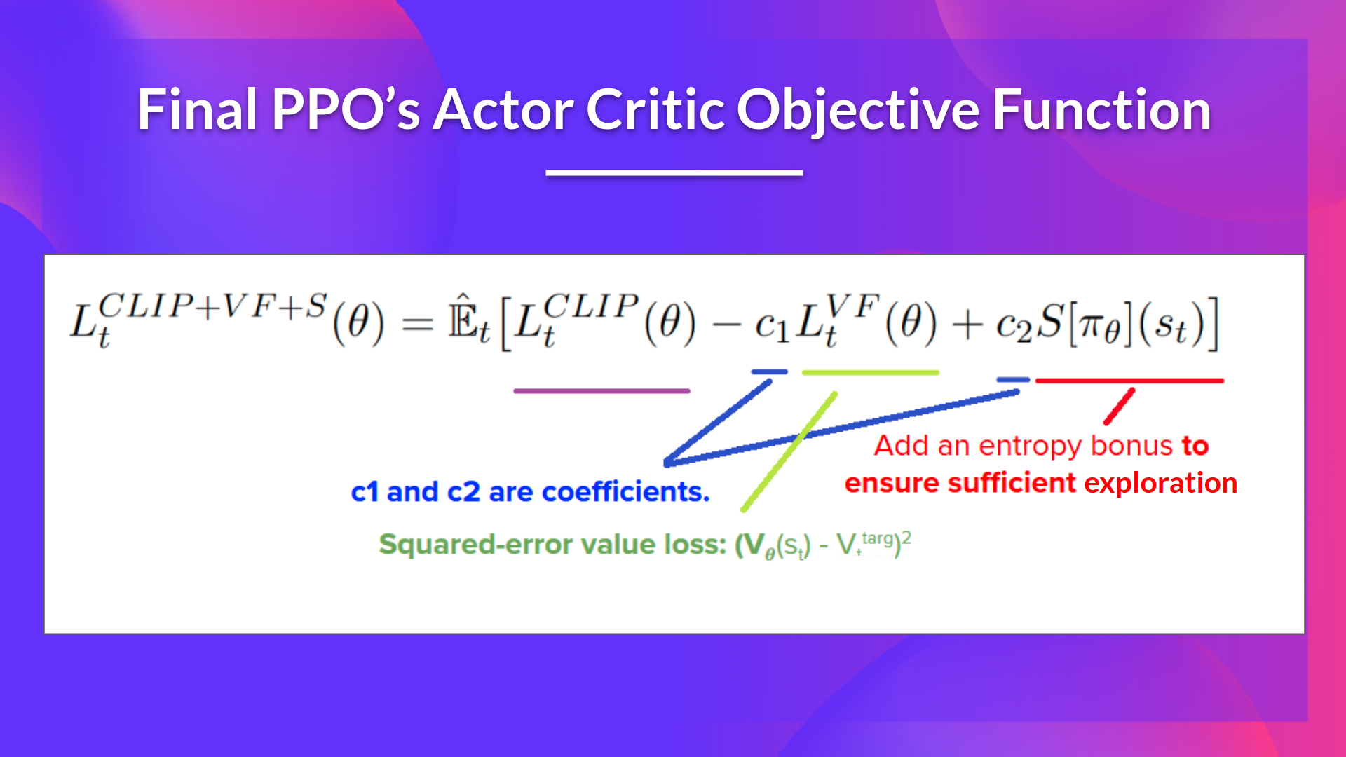
The final Clipped Surrogate Objective Loss for PPO Actor-Critic style looks like this, it’s a combination of Clipped Surrogate Objective function, Value Loss Function and Entropy bonus:
That was quite complex. Take time to understand these situations by looking at the table and the graph. You must understand why this makes sense. If you want to go deeper, the best resource is the article “Towards Delivering a Coherent Self-Contained Explanation of Proximal Policy Optimization” by Daniel Bick, especially part 3.4.
< > Update on GitHub