Diffusers documentation
Diffusion 모델 평가하기
Diffusion 모델 평가하기
Stable Diffusion와 같은 생성 모델의 평가는 주관적인 성격을 가지고 있습니다. 그러나 실무자와 연구자로서 우리는 종종 다양한 가능성 중에서 신중한 선택을 해야 합니다. 그래서 다양한 생성 모델 (GAN, Diffusion 등)을 사용할 때 어떻게 선택해야 할까요?
정성적인 평가는 모델의 이미지 품질에 대한 주관적인 평가이므로 오류가 발생할 수 있고 결정에 잘못된 영향을 미칠 수 있습니다. 반면, 정량적인 평가는 이미지 품질과 직접적인 상관관계를 갖지 않을 수 있습니다. 따라서 일반적으로 정성적 평가와 정량적 평가를 모두 고려하는 것이 더 강력한 신호를 제공하여 모델 선택에 도움이 됩니다.
이 문서에서는 Diffusion 모델을 평가하기 위한 정성적 및 정량적 방법에 대해 상세히 설명합니다. 정량적 방법에 대해서는 특히 diffusers와 함께 구현하는 방법에 초점을 맞추었습니다.
이 문서에서 보여진 방법들은 기반 생성 모델을 고정시키고 다양한 노이즈 스케줄러를 평가하는 데에도 사용할 수 있습니다.
시나리오
다음과 같은 파이프라인을 사용하여 Diffusion 모델을 다룹니다:
- 텍스트로 안내된 이미지 생성 (예:
StableDiffusionPipeline). - 입력 이미지에 추가로 조건을 건 텍스트로 안내된 이미지 생성 (예:
StableDiffusionImg2ImgPipeline및StableDiffusionInstructPix2PixPipeline). - 클래스 조건화된 이미지 생성 모델 (예:
DiTPipeline).
정성적 평가
정성적 평가는 일반적으로 생성된 이미지의 인간 평가를 포함합니다. 품질은 구성성, 이미지-텍스트 일치, 공간 관계 등과 같은 측면에서 측정됩니다. 일반적인 프롬프트는 주관적인 지표에 대한 일정한 기준을 제공합니다. DrawBench와 PartiPrompts는 정성적인 벤치마킹에 사용되는 프롬프트 데이터셋입니다. DrawBench와 PartiPrompts는 각각 Imagen과 Parti에서 소개되었습니다.
Parti 공식 웹사이트에서 다음과 같이 설명하고 있습니다:
PartiPrompts (P2)는 이 작업의 일부로 공개되는 영어로 된 1600개 이상의 다양한 프롬프트 세트입니다. P2는 다양한 범주와 도전 측면에서 모델의 능력을 측정하는 데 사용할 수 있습니다.
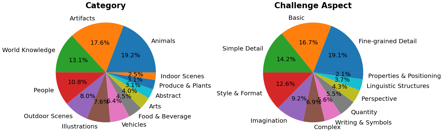
PartiPrompts는 다음과 같은 열을 가지고 있습니다:
- 프롬프트 (Prompt)
- 프롬프트의 카테고리 (예: “Abstract”, “World Knowledge” 등)
- 난이도를 반영한 챌린지 (예: “Basic”, “Complex”, “Writing & Symbols” 등)
이러한 벤치마크는 서로 다른 이미지 생성 모델을 인간 평가로 비교할 수 있도록 합니다.
이를 위해 🧨 Diffusers 팀은 Open Parti Prompts를 구축했습니다. 이는 Parti Prompts를 기반으로 한 커뮤니티 기반의 질적 벤치마크로, 최첨단 오픈 소스 확산 모델을 비교하는 데 사용됩니다:
- Open Parti Prompts 게임: 10개의 parti prompt에 대해 4개의 생성된 이미지가 제시되며, 사용자는 프롬프트에 가장 적합한 이미지를 선택합니다.
- Open Parti Prompts 리더보드: 현재 최고의 오픈 소스 diffusion 모델들을 서로 비교하는 리더보드입니다.
이미지를 수동으로 비교하려면, diffusers를 사용하여 몇가지 PartiPrompts를 어떻게 활용할 수 있는지 알아봅시다.
다음은 몇 가지 다른 도전에서 샘플링한 프롬프트를 보여줍니다: Basic, Complex, Linguistic Structures, Imagination, Writing & Symbols. 여기서는 PartiPrompts를 데이터셋으로 사용합니다.
from datasets import load_dataset

# prompts = load_dataset("nateraw/parti-prompts", split="train")
# prompts = prompts.shuffle()
# sample_prompts = [prompts[i]["Prompt"] for i in range(5)]

# Fixing these sample prompts in the interest of reproducibility.
sample_prompts = [
    "a corgi",
    "a hot air balloon with a yin-yang symbol, with the moon visible in the daytime sky",
    "a car with no windows",
    "a cube made of porcupine",
    'The saying "BE EXCELLENT TO EACH OTHER" written on a red brick wall with a graffiti image of a green alien wearing a tuxedo. A yellow fire hydrant is on a sidewalk in the foreground.',
]
이제 이런 프롬프트를 사용하여 Stable Diffusion (v1-4 checkpoint)를 사용한 이미지 생성을 할 수 있습니다 :
import torch

seed = 0
generator = torch.manual_seed(seed)

images = sd_pipeline(sample_prompts, num_images_per_prompt=1, generator=generator).images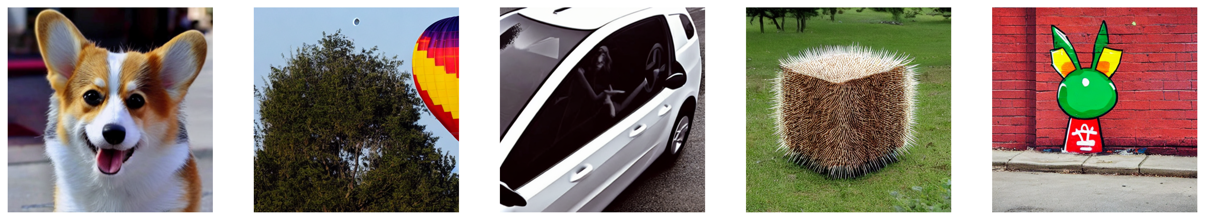
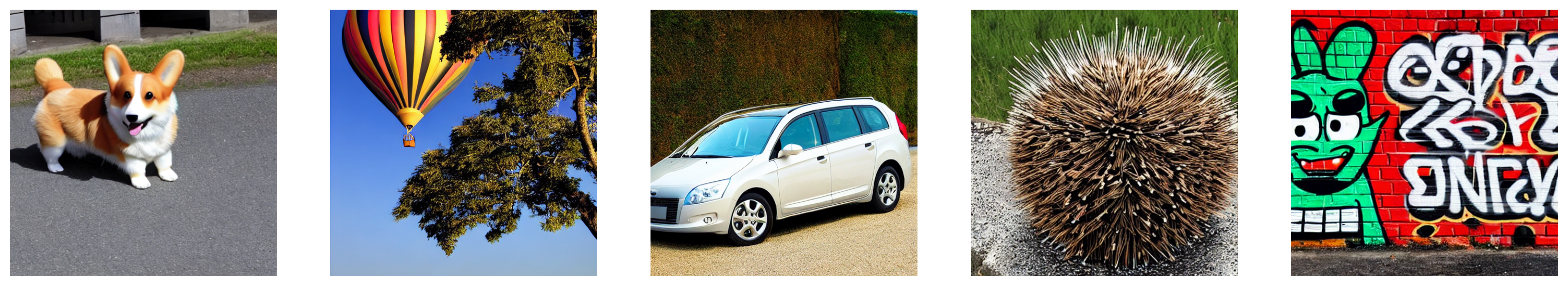
num_images_per_prompt를 설정하여 동일한 프롬프트에 대해 다른 이미지를 비교할 수도 있습니다. 다른 체크포인트(v1-5)로 동일한 파이프라인을 실행하면 다음과 같은 결과가 나옵니다:
다양한 모델을 사용하여 모든 프롬프트에서 생성된 여러 이미지들이 생성되면 (평가 과정에서) 이러한 결과물들은 사람 평가자들에게 점수를 매기기 위해 제시됩니다. DrawBench와 PartiPrompts 벤치마크에 대한 자세한 내용은 각각의 논문을 참조하십시오.
모델이 훈련 중일 때 추론 샘플을 살펴보는 것은 훈련 진행 상황을 측정하는 데 유용합니다. 훈련 스크립트에서는 TensorBoard와 Weights & Biases에 대한 추가 지원과 함께 이 유틸리티를 지원합니다.
정량적 평가
이 섹션에서는 세 가지 다른 확산 파이프라인을 평가하는 방법을 안내합니다:
- CLIP 점수
- CLIP 방향성 유사도
- FID
텍스트 안내 이미지 생성
CLIP 점수는 이미지-캡션 쌍의 호환성을 측정합니다. 높은 CLIP 점수는 높은 호환성🔼을 나타냅니다. CLIP 점수는 이미지와 캡션 사이의 의미적 유사성으로 생각할 수도 있습니다. CLIP 점수는 인간 판단과 높은 상관관계를 가지고 있습니다.
StableDiffusionPipeline을 일단 로드해봅시다:
from diffusers import StableDiffusionPipeline
import torch

model_ckpt = "CompVis/stable-diffusion-v1-4"
sd_pipeline = StableDiffusionPipeline.from_pretrained(model_ckpt, torch_dtype=torch.float16).to("cuda")
여러 개의 프롬프트를 사용하여 이미지를 생성합니다:
prompts = [
    "a photo of an astronaut riding a horse on mars",
    "A high tech solarpunk utopia in the Amazon rainforest",
    "A pikachu fine dining with a view to the Eiffel Tower",
    "A mecha robot in a favela in expressionist style",
    "an insect robot preparing a delicious meal",
    "A small cabin on top of a snowy mountain in the style of Disney, artstation",
]

images = sd_pipeline(prompts, num_images_per_prompt=1, output_type="np").images

print(images.shape)
# (6, 512, 512, 3)
그러고 나서 CLIP 점수를 계산합니다.
from torchmetrics.functional.multimodal import clip_score
from functools import partial

clip_score_fn = partial(clip_score, model_name_or_path="openai/clip-vit-base-patch16")

def calculate_clip_score(images, prompts):
    images_int = (images * 255).astype("uint8")
    clip_score = clip_score_fn(torch.from_numpy(images_int).permute(0, 3, 1, 2), prompts).detach()
    return round(float(clip_score), 4)

sd_clip_score = calculate_clip_score(images, prompts)
print(f"CLIP score: {sd_clip_score}")
# CLIP score: 35.7038
위의 예제에서는 각 프롬프트 당 하나의 이미지를 생성했습니다. 만약 프롬프트 당 여러 이미지를 생성한다면, 프롬프트 당 생성된 이미지의 평균 점수를 사용해야 합니다.
이제 StableDiffusionPipeline과 호환되는 두 개의 체크포인트를 비교하려면, 파이프라인을 호출할 때 generator를 전달해야 합니다. 먼저, 고정된 시드로 v1-4 Stable Diffusion 체크포인트를 사용하여 이미지를 생성합니다:
seed = 0
generator = torch.manual_seed(seed)

images = sd_pipeline(prompts, num_images_per_prompt=1, generator=generator, output_type="np").images
그런 다음 v1-5 checkpoint를 로드하여 이미지를 생성합니다:
model_ckpt_1_5 = "runwayml/stable-diffusion-v1-5"
sd_pipeline_1_5 = StableDiffusionPipeline.from_pretrained(model_ckpt_1_5, torch_dtype=weight_dtype).to(device)

images_1_5 = sd_pipeline_1_5(prompts, num_images_per_prompt=1, generator=generator, output_type="np").images
그리고 마지막으로 CLIP 점수를 비교합니다:
sd_clip_score_1_4 = calculate_clip_score(images, prompts)
print(f"CLIP Score with v-1-4: {sd_clip_score_1_4}")
# CLIP Score with v-1-4: 34.9102

sd_clip_score_1_5 = calculate_clip_score(images_1_5, prompts)
print(f"CLIP Score with v-1-5: {sd_clip_score_1_5}")
# CLIP Score with v-1-5: 36.2137
v1-5 체크포인트가 이전 버전보다 더 나은 성능을 보이는 것 같습니다. 그러나 CLIP 점수를 계산하기 위해 사용한 프롬프트의 수가 상당히 적습니다. 보다 실용적인 평가를 위해서는 이 수를 훨씬 높게 설정하고, 프롬프트를 다양하게 사용해야 합니다.
이 점수에는 몇 가지 제한 사항이 있습니다. 훈련 데이터셋의 캡션은 웹에서 크롤링되어 이미지와 관련된 alt 및 유사한 태그에서 추출되었습니다. 이들은 인간이 이미지를 설명하는 데 사용할 수 있는 것과 일치하지 않을 수 있습니다. 따라서 여기서는 몇 가지 프롬프트를 “엔지니어링”해야 했습니다.
이미지 조건화된 텍스트-이미지 생성
이 경우, 생성 파이프라인을 입력 이미지와 텍스트 프롬프트로 조건화합니다. StableDiffusionInstructPix2PixPipeline을 예로 들어보겠습니다. 이는 편집 지시문을 입력 프롬프트로 사용하고 편집할 입력 이미지를 사용합니다.
다음은 하나의 예시입니다:
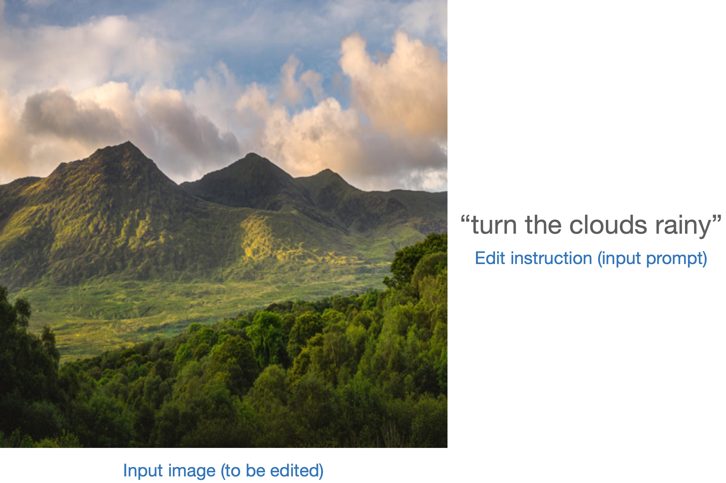
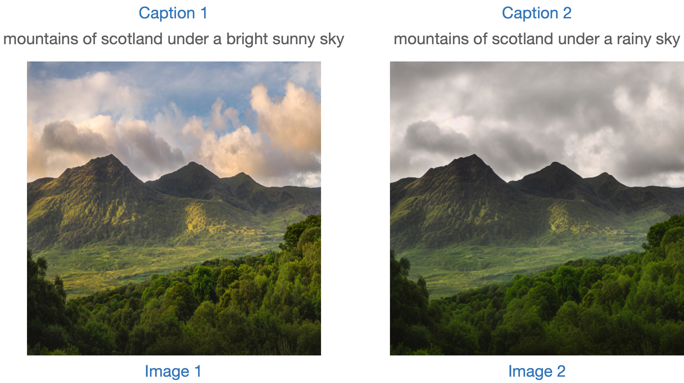
모델을 평가하는 한 가지 전략은 두 이미지 캡션 간의 변경과(CLIP-Guided Domain Adaptation of Image Generators에서 보여줍니다) 함께 두 이미지 사이의 변경의 일관성을 측정하는 것입니다 (CLIP 공간에서). 이를 ”CLIP 방향성 유사성“이라고 합니다.
- 캡션 1은 편집할 이미지 (이미지 1)에 해당합니다.
- 캡션 2는 편집된 이미지 (이미지 2)에 해당합니다. 편집 지시를 반영해야 합니다.
다음은 그림으로 된 개요입니다:
우리는 이 측정 항목을 구현하기 위해 미니 데이터 세트를 준비했습니다. 먼저 데이터 세트를 로드해 보겠습니다.
from datasets import load_dataset

dataset = load_dataset("sayakpaul/instructpix2pix-demo", split="train")
dataset.features{'input': Value(dtype='string', id=None),
'edit': Value(dtype='string', id=None),
'output': Value(dtype='string', id=None),
'image': Image(decode=True, id=None)}여기에는 다음과 같은 항목이 있습니다:
input은image에 해당하는 캡션입니다.edit은 편집 지시사항을 나타냅니다.output은edit지시사항을 반영한 수정된 캡션입니다.
샘플을 살펴보겠습니다.
idx = 0
print(f"Original caption: {dataset[idx]['input']}")
print(f"Edit instruction: {dataset[idx]['edit']}")
print(f"Modified caption: {dataset[idx]['output']}")Original caption: 2. FAROE ISLANDS: An archipelago of 18 mountainous isles in the North Atlantic Ocean between Norway and Iceland, the Faroe Islands has 'everything you could hope for', according to Big 7 Travel. It boasts 'crystal clear waterfalls, rocky cliffs that seem to jut out of nowhere and velvety green hills'
Edit instruction: make the isles all white marble
Modified caption: 2. WHITE MARBLE ISLANDS: An archipelago of 18 mountainous white marble isles in the North Atlantic Ocean between Norway and Iceland, the White Marble Islands has 'everything you could hope for', according to Big 7 Travel. It boasts 'crystal clear waterfalls, rocky cliffs that seem to jut out of nowhere and velvety green hills'다음은 이미지입니다:
dataset[idx]["image"]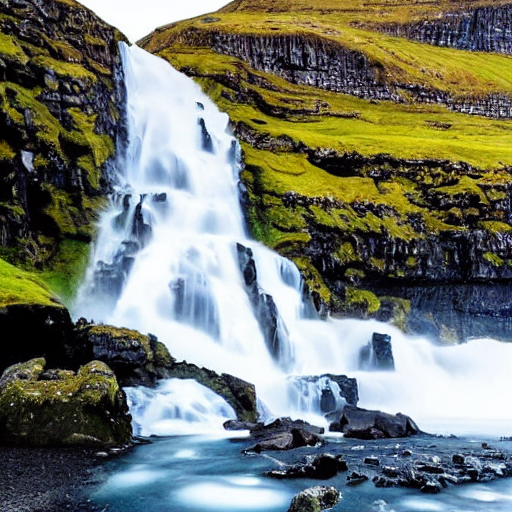
먼저 편집 지시사항을 사용하여 데이터 세트의 이미지를 편집하고 방향 유사도를 계산합니다.
StableDiffusionInstructPix2PixPipeline를 먼저 로드합니다:
from diffusers import StableDiffusionInstructPix2PixPipeline

instruct_pix2pix_pipeline = StableDiffusionInstructPix2PixPipeline.from_pretrained(
    "timbrooks/instruct-pix2pix", torch_dtype=torch.float16
).to(device)
이제 편집을 수행합니다:
import numpy as np


def edit_image(input_image, instruction):
    image = instruct_pix2pix_pipeline(
        instruction,
        image=input_image,
        output_type="np",
        generator=generator,
    ).images[0]
    return image

input_images = []
original_captions = []
modified_captions = []
edited_images = []

for idx in range(len(dataset)):
    input_image = dataset[idx]["image"]
    edit_instruction = dataset[idx]["edit"]
    edited_image = edit_image(input_image, edit_instruction)

    input_images.append(np.array(input_image))
    original_captions.append(dataset[idx]["input"])
    modified_captions.append(dataset[idx]["output"])
    edited_images.append(edited_image)
방향 유사도를 계산하기 위해서는 먼저 CLIP의 이미지와 텍스트 인코더를 로드합니다:
from transformers import (
    CLIPTokenizer,
    CLIPTextModelWithProjection,
    CLIPVisionModelWithProjection,
    CLIPImageProcessor,
)

clip_id = "openai/clip-vit-large-patch14"
tokenizer = CLIPTokenizer.from_pretrained(clip_id)
text_encoder = CLIPTextModelWithProjection.from_pretrained(clip_id).to(device)
image_processor = CLIPImageProcessor.from_pretrained(clip_id)
image_encoder = CLIPVisionModelWithProjection.from_pretrained(clip_id).to(device)
주목할 점은 특정한 CLIP 체크포인트인 openai/clip-vit-large-patch14를 사용하고 있다는 것입니다. 이는 Stable Diffusion 사전 훈련이 이 CLIP 변형체와 함께 수행되었기 때문입니다. 자세한 내용은 문서를 참조하세요.
다음으로, 방향성 유사도를 계산하기 위해 PyTorch의 nn.Module을 준비합니다:
import torch.nn as nn
import torch.nn.functional as F


class DirectionalSimilarity(nn.Module):
    def __init__(self, tokenizer, text_encoder, image_processor, image_encoder):
        super().__init__()
        self.tokenizer = tokenizer
        self.text_encoder = text_encoder
        self.image_processor = image_processor
        self.image_encoder = image_encoder

    def preprocess_image(self, image):
        image = self.image_processor(image, return_tensors="pt")["pixel_values"]
        return {"pixel_values": image.to(device)}

    def tokenize_text(self, text):
        inputs = self.tokenizer(
            text,
            max_length=self.tokenizer.model_max_length,
            padding="max_length",
            truncation=True,
            return_tensors="pt",
        )
        return {"input_ids": inputs.input_ids.to(device)}

    def encode_image(self, image):
        preprocessed_image = self.preprocess_image(image)
        image_features = self.image_encoder(**preprocessed_image).image_embeds
        image_features = image_features / image_features.norm(dim=1, keepdim=True)
        return image_features

    def encode_text(self, text):
        tokenized_text = self.tokenize_text(text)
        text_features = self.text_encoder(**tokenized_text).text_embeds
        text_features = text_features / text_features.norm(dim=1, keepdim=True)
        return text_features

    def compute_directional_similarity(self, img_feat_one, img_feat_two, text_feat_one, text_feat_two):
        sim_direction = F.cosine_similarity(img_feat_two - img_feat_one, text_feat_two - text_feat_one)
        return sim_direction

    def forward(self, image_one, image_two, caption_one, caption_two):
        img_feat_one = self.encode_image(image_one)
        img_feat_two = self.encode_image(image_two)
        text_feat_one = self.encode_text(caption_one)
        text_feat_two = self.encode_text(caption_two)
        directional_similarity = self.compute_directional_similarity(
            img_feat_one, img_feat_two, text_feat_one, text_feat_two
        )
        return directional_similarity
이제 DirectionalSimilarity를 사용해 보겠습니다.
dir_similarity = DirectionalSimilarity(tokenizer, text_encoder, image_processor, image_encoder)
scores = []

for i in range(len(input_images)):
    original_image = input_images[i]
    original_caption = original_captions[i]
    edited_image = edited_images[i]
    modified_caption = modified_captions[i]

    similarity_score = dir_similarity(original_image, edited_image, original_caption, modified_caption)
    scores.append(float(similarity_score.detach().cpu()))

print(f"CLIP directional similarity: {np.mean(scores)}")
# CLIP directional similarity: 0.0797976553440094
CLIP 점수와 마찬가지로, CLIP 방향 유사성이 높을수록 좋습니다.
StableDiffusionInstructPix2PixPipeline은 image_guidance_scale과 guidance_scale이라는 두 가지 인자를 노출시킵니다. 이 두 인자를 조정하여 최종 편집된 이미지의 품질을 제어할 수 있습니다. 이 두 인자의 영향을 실험해보고 방향 유사성에 미치는 영향을 확인해보기를 권장합니다.
이러한 메트릭의 개념을 확장하여 원본 이미지와 편집된 버전의 유사성을 측정할 수 있습니다. 이를 위해 F.cosine_similarity(img_feat_two, img_feat_one)을 사용할 수 있습니다. 이러한 종류의 편집에서는 이미지의 주요 의미가 최대한 보존되어야 합니다. 즉, 높은 유사성 점수를 얻어야 합니다.
StableDiffusionPix2PixZeroPipeline와 같은 유사한 파이프라인에도 이러한 메트릭을 사용할 수 있습니다.
CLIP 점수와 CLIP 방향 유사성 모두 CLIP 모델에 의존하기 때문에 평가가 편향될 수 있습니다
IS, FID (나중에 설명할 예정), 또는 KID와 같은 메트릭을 확장하는 것은 어려울 수 있습니다. 평가 중인 모델이 대규모 이미지 캡셔닝 데이터셋 (예: LAION-5B 데이터셋)에서 사전 훈련되었을 때 이는 문제가 될 수 있습니다. 왜냐하면 이러한 메트릭의 기반에는 중간 이미지 특징을 추출하기 위해 ImageNet-1k 데이터셋에서 사전 훈련된 InceptionNet이 사용되기 때문입니다. Stable Diffusion의 사전 훈련 데이터셋은 InceptionNet의 사전 훈련 데이터셋과 겹치는 부분이 제한적일 수 있으므로 따라서 여기에는 좋은 후보가 아닙니다.
위의 메트릭을 사용하면 클래스 조건이 있는 모델을 평가할 수 있습니다. 예를 들어, DiT. 이는 ImageNet-1k 클래스에 조건을 걸고 사전 훈련되었습니다.
클래스 조건화 이미지 생성
클래스 조건화 생성 모델은 일반적으로 ImageNet-1k와 같은 클래스 레이블이 지정된 데이터셋에서 사전 훈련됩니다. 이러한 모델을 평가하는 인기있는 지표에는 Fréchet Inception Distance (FID), Kernel Inception Distance (KID) 및 Inception Score (IS)가 있습니다. 이 문서에서는 FID (Heusel et al.)에 초점을 맞추고 있습니다. DiTPipeline을 사용하여 FID를 계산하는 방법을 보여줍니다. 이는 내부적으로 DiT 모델을 사용합니다.
FID는 두 개의 이미지 데이터셋이 얼마나 유사한지를 측정하는 것을 목표로 합니다. 이 자료에 따르면:
Fréchet Inception Distance는 두 개의 이미지 데이터셋 간의 유사성을 측정하는 지표입니다. 시각적 품질에 대한 인간 판단과 잘 상관되는 것으로 나타났으며, 주로 생성적 적대 신경망의 샘플 품질을 평가하는 데 사용됩니다. FID는 Inception 네트워크의 특징 표현에 맞게 적합한 두 개의 가우시안 사이의 Fréchet 거리를 계산하여 구합니다.
이 두 개의 데이터셋은 실제 이미지 데이터셋과 가짜 이미지 데이터셋(우리의 경우 생성된 이미지)입니다. FID는 일반적으로 두 개의 큰 데이터셋으로 계산됩니다. 그러나 이 문서에서는 두 개의 미니 데이터셋으로 작업할 것입니다.
먼저 ImageNet-1k 훈련 세트에서 몇 개의 이미지를 다운로드해 봅시다:
from zipfile import ZipFile
import requests


def download(url, local_filepath):
    r = requests.get(url)
    with open(local_filepath, "wb") as f:
        f.write(r.content)
    return local_filepath

dummy_dataset_url = "https://hf.co/datasets/sayakpaul/sample-datasets/resolve/main/sample-imagenet-images.zip"
local_filepath = download(dummy_dataset_url, dummy_dataset_url.split("/")[-1])

with ZipFile(local_filepath, "r") as zipper:
zipper.extractall(".")from PIL import Image
import os
dataset_path = "sample-imagenet-images"
image_paths = sorted([os.path.join(dataset_path, x) for x in os.listdir(dataset_path)])
real_images = [np.array(Image.open(path).convert("RGB")) for path in image_paths]다음은 ImageNet-1k classes의 이미지 10개입니다 : “cassette_player”, “chain_saw” (x2), “church”, “gas_pump” (x3), “parachute” (x2), 그리고 “tench”.
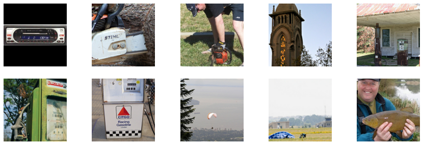
Real images.
이제 이미지가 로드되었으므로 이미지에 가벼운 전처리를 적용하여 FID 계산에 사용해 보겠습니다.
from torchvision.transforms import functional as F


def preprocess_image(image):
    image = torch.tensor(image).unsqueeze(0)
    image = image.permute(0, 3, 1, 2) / 255.0
    return F.center_crop(image, (256, 256))

real_images = torch.cat([preprocess_image(image) for image in real_images])
print(real_images.shape)
# torch.Size([10, 3, 256, 256])
이제 위에서 언급한 클래스에 따라 조건화 된 이미지를 생성하기 위해 DiTPipeline를 로드합니다.
from diffusers import DiTPipeline, DPMSolverMultistepScheduler

dit_pipeline = DiTPipeline.from_pretrained("facebook/DiT-XL-2-256", torch_dtype=torch.float16)
dit_pipeline.scheduler = DPMSolverMultistepScheduler.from_config(dit_pipeline.scheduler.config)
dit_pipeline = dit_pipeline.to("cuda")

words = [
    "cassette player",
    "chainsaw",
    "chainsaw",
    "church",
    "gas pump",
    "gas pump",
    "gas pump",
    "parachute",
    "parachute",
    "tench",
]

class_ids = dit_pipeline.get_label_ids(words)
output = dit_pipeline(class_labels=class_ids, generator=generator, output_type="np")

fake_images = output.images
fake_images = torch.tensor(fake_images)
fake_images = fake_images.permute(0, 3, 1, 2)
print(fake_images.shape)
# torch.Size([10, 3, 256, 256])
이제 torchmetrics를 사용하여 FID를 계산할 수 있습니다.
from torchmetrics.image.fid import FrechetInceptionDistance

fid = FrechetInceptionDistance(normalize=True)
fid.update(real_images, real=True)
fid.update(fake_images, real=False)

print(f"FID: {float(fid.compute())}")
# FID: 177.7147216796875
FID는 낮을수록 좋습니다. 여러 가지 요소가 FID에 영향을 줄 수 있습니다:
- 이미지의 수 (실제 이미지와 가짜 이미지 모두)
- diffusion 과정에서 발생하는 무작위성
- diffusion 과정에서의 추론 단계 수
- diffusion 과정에서 사용되는 스케줄러
마지막 두 가지 요소에 대해서는, 다른 시드와 추론 단계에서 평가를 실행하고 평균 결과를 보고하는 것은 좋은 실천 방법입니다
FID 결과는 많은 요소에 의존하기 때문에 취약할 수 있습니다:
- 계산 중 사용되는 특정 Inception 모델.
- 계산의 구현 정확도.
- 이미지 형식 (PNG 또는 JPG에서 시작하는 경우가 다릅니다).
이러한 사항을 염두에 두면, FID는 유사한 실행을 비교할 때 가장 유용하지만, 저자가 FID 측정 코드를 주의 깊게 공개하지 않는 한 논문 결과를 재현하기는 어렵습니다.
이러한 사항은 KID 및 IS와 같은 다른 관련 메트릭에도 적용됩니다.
마지막 단계로, fake_images를 시각적으로 검사해 봅시다.
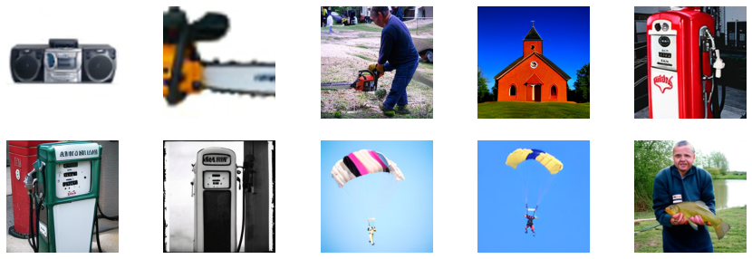
Fake images.