Self-Play: a classic technique to train competitive agents in adversarial games
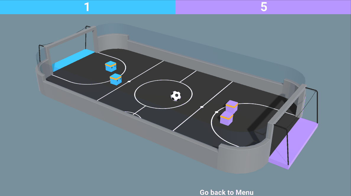
Now that we’ve studied the basics of multi-agents, we’re ready to go deeper. As mentioned in the introduction, we’re going to train agents in an adversarial game with SoccerTwos, a 2vs2 game.
What is Self-Play?
Training agents correctly in an adversarial game can be quite complex.
On the one hand, we need to find how to get a well-trained opponent to play against your training agent. And on the other hand, if you find a very good trained opponent, how will your agent improve its policy when the opponent is too strong?
Think of a child that just started to learn soccer. Playing against a very good soccer player will be useless since it will be too hard to win or at least get the ball from time to time. So the child will continuously lose without having time to learn a good policy.
The best solution would be to have an opponent that is on the same level as the agent and will upgrade its level as the agent upgrades its own. Because if the opponent is too strong, we’ll learn nothing; if it is too weak, we’ll overlearn useless behavior against a stronger opponent then.
This solution is called self-play. In self-play, the agent uses former copies of itself (of its policy) as an opponent. This way, the agent will play against an agent of the same level (challenging but not too much), have opportunities to gradually improve its policy, and then update its opponent as it becomes better. It’s a way to bootstrap an opponent and progressively increase the opponent’s complexity.
It’s the same way humans learn in competition:
- We start to train against an opponent of similar level
- Then we learn from it, and when we acquire some skills, we can move further with stronger opponents.
We do the same with self-play:
- We start with a copy of our agent as an opponent this way, this opponent is on a similar level.
- We learn from it and, when we acquire some skills, we update our opponent with a more recent copy of our training policy.
The theory behind self-play is not something new. It was already used by Arthur Samuel’s checker player system in the fifties and by Gerald Tesauro’s TD-Gammon in 1995. If you want to learn more about the history of self-play check out this very good blogpost by Andrew Cohen
Self-Play in MLAgents
Self-Play is integrated into the MLAgents library and is managed by multiple hyperparameters that we’re going to study. But the main focus, as explained in the documentation, is the tradeoff between the skill level and generality of the final policy and the stability of learning.
Training against a set of slowly changing or unchanging adversaries with low diversity results in more stable training. But a risk to overfit if the change is too slow.
So we need to control:
- How often we change opponents with the
swap_stepsandteam_changeparameters. - The number of opponents saved with the
windowparameter. A larger value ofwindowmeans that an agent’s pool of opponents will contain a larger diversity of behaviors since it will contain policies from earlier in the training run. - The probability of playing against the current self vs opponent sampled from the pool with
play_against_latest_model_ratio. A larger value ofplay_against_latest_model_ratioindicates that an agent will be playing against the current opponent more often. - The number of training steps before saving a new opponent with
save_stepsparameters. A larger value ofsave_stepswill yield a set of opponents that cover a wider range of skill levels and possibly play styles since the policy receives more training.
To get more details about these hyperparameters, you definitely need to check out this part of the documentation
The ELO Score to evaluate our agent
What is ELO Score?
In adversarial games, tracking the cumulative reward is not always a meaningful metric to track the learning progress: because this metric is dependent only on the skill of the opponent.
Instead, we’re using an ELO rating system (named after Arpad Elo) that calculates the relative skill level between 2 players from a given population in a zero-sum game.
In a zero-sum game: one agent wins, and the other agent loses. It’s a mathematical representation of a situation in which each participant’s gain or loss of utility is exactly balanced by the gain or loss of the utility of the other participants. We talk about zero-sum games because the sum of utility is equal to zero.
This ELO (starting at a specific score: frequently 1200) can decrease initially but should increase progressively during the training.
The Elo system is inferred from the losses and draws against other players. It means that player ratings depend on the ratings of their opponents and the results scored against them.
Elo defines an Elo score that is the relative skills of a player in a zero-sum game. We say relative because it depends on the performance of opponents.
The central idea is to think of the performance of a player as a random variable that is normally distributed.
The difference in rating between 2 players serves as the predictor of the outcomes of a match. If the player wins, but the probability of winning is high, it will only win a few points from its opponent since it means that it is much stronger than it.
After every game:
- The winning player takes points from the losing one.
- The number of points is determined by the difference in the 2 players ratings (hence relative).
- If the higher-rated player wins → few points will be taken from the lower-rated player.
- If the lower-rated player wins → a lot of points will be taken from the high-rated player.
- If it’s a draw → the lower-rated player gains a few points from the higher.
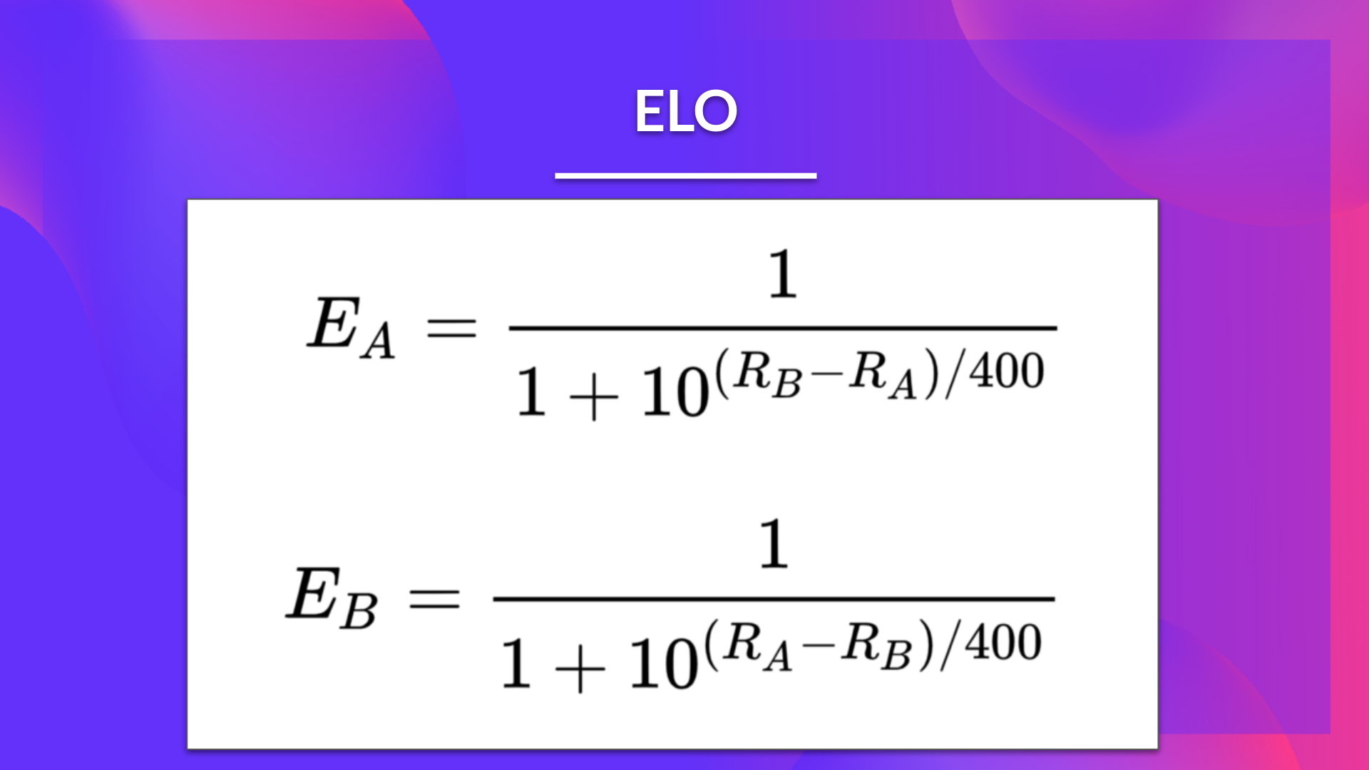
So if A and B have rating Ra, and Rb, then the expected scores are given by:
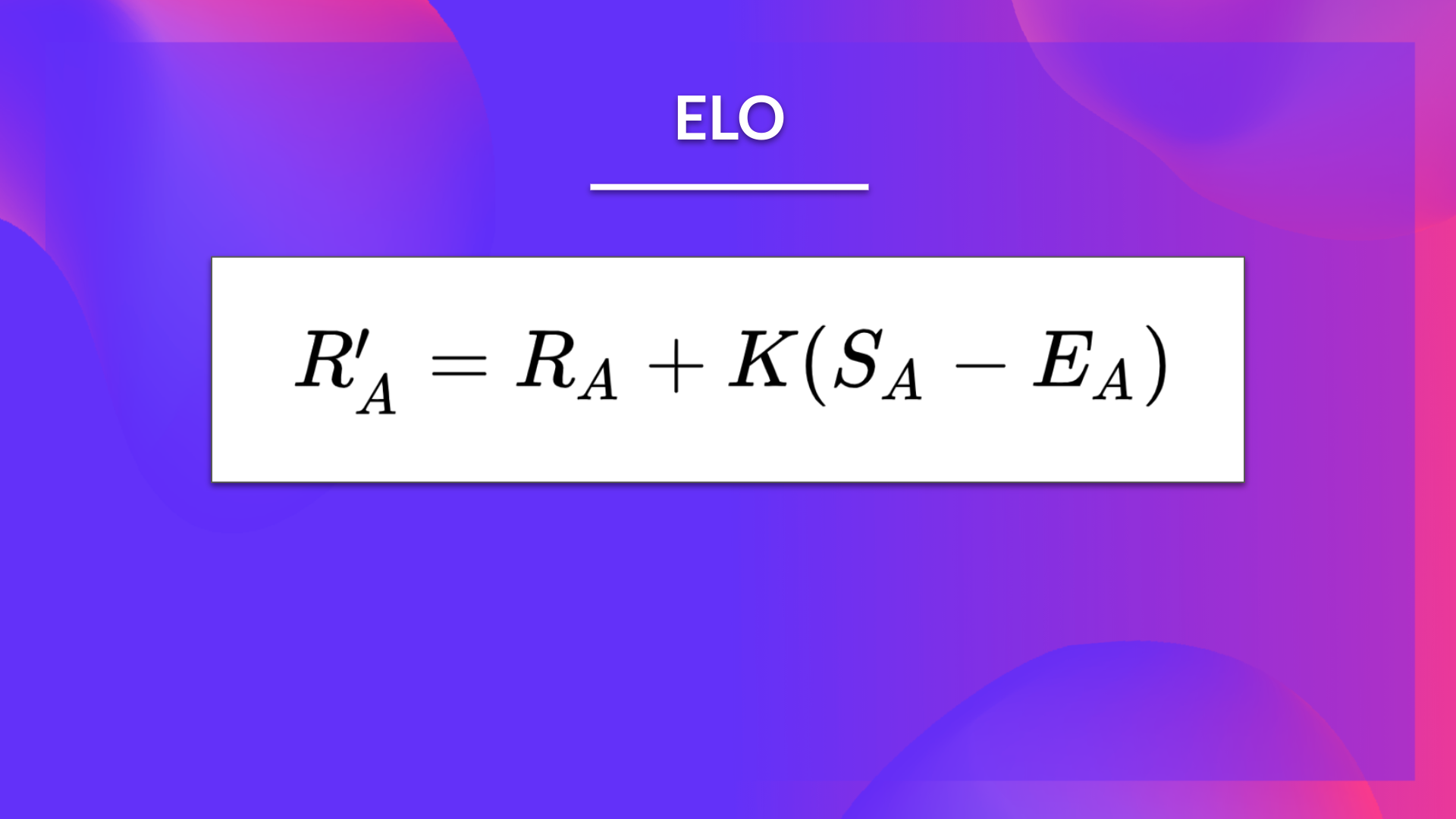
Then, at the end of the game, we need to update the player’s actual Elo score. We use a linear adjustment proportional to the amount by which the player over-performed or under-performed.
We also define a maximum adjustment rating per game: K-factor.
- K=16 for master.
- K=32 for weaker players.
If Player A has Ea points but scored Sa points, then the player’s rating is updated using the formula:
Example
If we take an example:
Player A has a rating of 2600
Player B has a rating of 2300
We first calculate the expected score:
If the organizers determined that K=16 and A wins, the new rating would be:
If the organizers determined that K=16 and B wins, the new rating would be:
The Advantages
Using the ELO score has multiple advantages:
- Points are always balanced (more points are exchanged when there is an unexpected outcome, but the sum is always the same).
- It is a self-corrected system since if a player wins against a weak player, they will only win a few points.
- It works with team games: we calculate the average for each team and use it in Elo.
The Disadvantages
- ELO does not take into account the individual contribution of each people in the team.
- Rating deflation: a good rating requires skill over time to keep the same rating.
- Can’t compare rating in history.