
license: cc-by-sa-4.0
pretty_name: Weight Systems Defining Five-Dimensional IP Lattice Polytopes
configs:
  - config_name: non-reflexive
    data_files:
      - split: full
        path: non-reflexive/*.parquet
  - config_name: reflexive
    data_files:
      - split: full
        path: reflexive/*.parquet
size_categories:
  - 100B<n<1T
tags:
  - physics
  - math
Weight Systems Defining Five-Dimensional IP Lattice Polytopes
This dataset contains all weight systems defining five-dimensional reflexive and non-reflexive IP lattice polytopes, instrumental in the study of Calabi-Yau fourfolds in mathematics and theoretical physics. The data was compiled by Harald Skarke and Friedrich Schöller in arXiv:1808.02422. More information is available at the Calabi-Yau data website. The dataset can be explored using the search frontend. See below for a short mathematical exposition on the construction of polytopes.
Please cite the paper when referencing this dataset:
@article{Scholler:2018apc,
    author = {Schöller, Friedrich and Skarke, Harald},
    title = "{All Weight Systems for Calabi-Yau Fourfolds from Reflexive Polyhedra}",
    eprint = "1808.02422",
    archivePrefix = "arXiv",
    primaryClass = "hep-th",
    doi = "10.1007/s00220-019-03331-9",
    journal = "Commun. Math. Phys.",
    volume = "372",
    number = "2",
    pages = "657--678",
    year = "2019"
}
Dataset Details
The dataset consists of two subsets: weight systems defining reflexive (and therefore IP) polytopes and weight systems defining non-reflexive IP polytopes. Each subset is split into 4000 files in Parquet format. Rows within each file are sorted lexicographically by weights. There are 185,269,499,015 weight systems defining reflexive polytopes and 137,114,261,915 defining non-reflexive polytopes, making a total of 322,383,760,930 IP weight systems.
Each row in the dataset represents a polytope and contains the six weights defining it, along with the vertex count, facet count, and lattice point count. The reflexive dataset also includes the Hodge numbers , , and of the corresponding Calabi-Yau manifold, and the lattice point count of the dual polytope.
For any Calabi-Yau fourfold, the Euler characteristic and the Hodge number can be derived as follows:
This dataset is licensed under the CC BY-SA 4.0 license.
Data Fields
weight0toweight5: Weights of the weight system defining the polytope.vertex_count: Vertex count of the polytope.facet_count: Facet count of the polytope.point_count: Lattice point count of the polytope.dual_point_count: Lattice point count of the dual polytope (only for reflexive polytopes).h11: Hodge number (only for reflexive polytopes).h12: Hodge number (only for reflexive polytopes).h13: Hodge number (only for reflexive polytopes).
Usage
The dataset can be used without downloading it entirely, thanks to the streaming
capability of the datasets library. The following Python code snippet demonstrates how
to stream the dataset and print the first five rows:
from datasets import load_dataset

dataset = load_dataset("calabi-yau-data/ws-5d", name="reflexive", split="full", streaming=True)

for row in dataset.take(5):
    print(row)
When cloning the Git repository with Git Large File Storage (LFS), data files are stored both in the Git LFS storage directory and in the working tree. To avoid occupying double the disk space, use a filesystem that supports copy-on-write, and run the following commands to clone the repository:
# Initialize Git LFS
git lfs install

# Clone the repository without downloading LFS files immediately
GIT_LFS_SKIP_SMUDGE=1 git clone https://huggingface.co/datasets/calabi-yau-data/ws-5d

# Change to the repository directory
cd ws-5d

# Test deduplication (optional)
git lfs dedup --test

# Download the LFS files
git lfs fetch

# Create working tree files as clones of the files in the Git LFS storage directory using
# copy-on-write functionality
git lfs dedup
Construction of Polytopes
This is an introduction to the mathematics involved in the construction of polytopes relevant to this dataset. For more details and precise definitions, consult the paper arXiv:1808.02422 and references therein.
Polytopes
A polytope is the convex hull of a finite set of points in -dimensional Euclidean space, . This means it is the smallest convex shape that contains all these points. The minimal collection of points that define a particular polytope are its vertices. Familiar examples of polytopes include triangles and rectangles in two dimensions, and cubes and octahedra in three dimensions.
A polytope is considered an IP polytope (interior point polytope) if the origin of is in the interior of the polytope, not on its boundary or outside it.
For any IP polytope , its dual polytope is defined as the set of points satisfying
This relationship is symmetric: the dual of the dual of an IP polytope is the polytope itself, i.e., .
Weight Systems
Weight systems provide a means to describe simple polytopes known as simplices. A weight system is a tuple of real numbers. The construction process is outlined as follows:
Consider an -dimensional simplex in , i.e., a polytope in with vertex count and of its edges extending in linearly independent directions. It is possible to position of its vertices at arbitrary (linearly independent) locations through a linear transformation. The placement of the remaining vertex is then determined. Its position is the defining property of the simplex. To specify the position independently of the applied linear transformation, one can use the following equation. If are the vertices of the simplex, this relation fixes one vertex in terms of the other :
where is the tuple of real numbers, the weight system.
It is important to note that scaling all weights in a weight system by a common factor results in an equivalent weight system that defines the same simplex.
The condition that a simplex is an IP simplex is equivalent to the condition that all weights in its weight system are bigger than zero.
For this dataset, the focus is on a specific construction of lattice polytopes described in subsequent sections.
Lattice Polytopes
A lattice polytope is a polytope with vertices at the points of a regular grid, or lattice. Using linear transformations, any lattice polytope can be transformed so that its vertices have integer coordinates, hence they are also referred to as integral polytopes.
The dual of a lattice with points is the lattice consisting of all points that satisfy
Reflexive polytopes are a specific type of lattice polytope characterized by having a dual that is also a lattice polytope, with vertices situated on the dual lattice. These polytopes play a central role in the context of this dataset.
The weights of a lattice polytope are always rational. This characteristic enables the rescaling of a weight system so that its weights become integers without any common divisor. This rescaling has been performed in this dataset.
The construction of the lattice polytopes from this dataset works as follows: We start with the simplex , arising from a weight system as previously described. Then, we define the polytope as the convex hull of the intersection of with the points of the dual lattice. In the context of this dataset, the polytope is referred to as ‘the polytope’. Correspondingly, is referred to as ‘the dual polytope’. The lattice of and is taken to be the coarsest lattice possible, such that is a lattice polytope, i.e., the lattice generated by the vertices of . This construction is exemplified in the following sections.
A weight system is considered an IP weight system if the corresponding is an IP polytope; that is, the origin is within its interior. Since only IP polytopes have corresponding dual polytopes, this condition is essential for the polytope to be classified as reflexive.
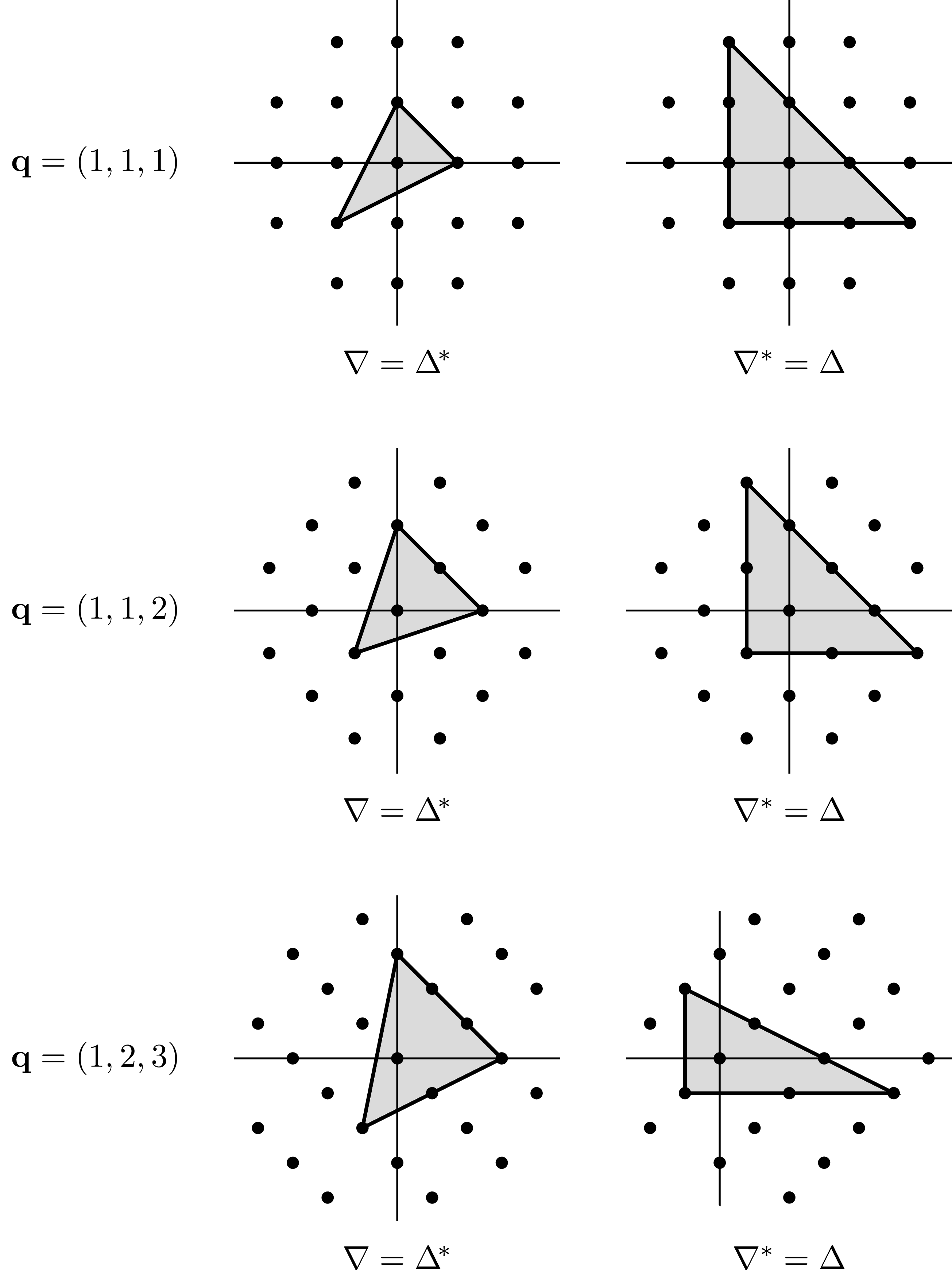
Two Dimensions
In two dimensions, all IP weight systems define reflexive polytopes and every vertex of lies on the dual lattice, making and identical. There are exactly three IP weight systems that define two-dimensional polytopes (polygons). Each polytope is reflexive and has three vertices and three facets (edges):
| weight system | number of points of | number of points of |
|---|---|---|
| (1, 1, 1) | 4 | 10 |
| (1, 1, 2) | 5 | 9 |
| (1, 2, 3) | 7 | 7 |
The polytopes and their duals are depicted below. Lattice points are indicated by dots.
General Dimension
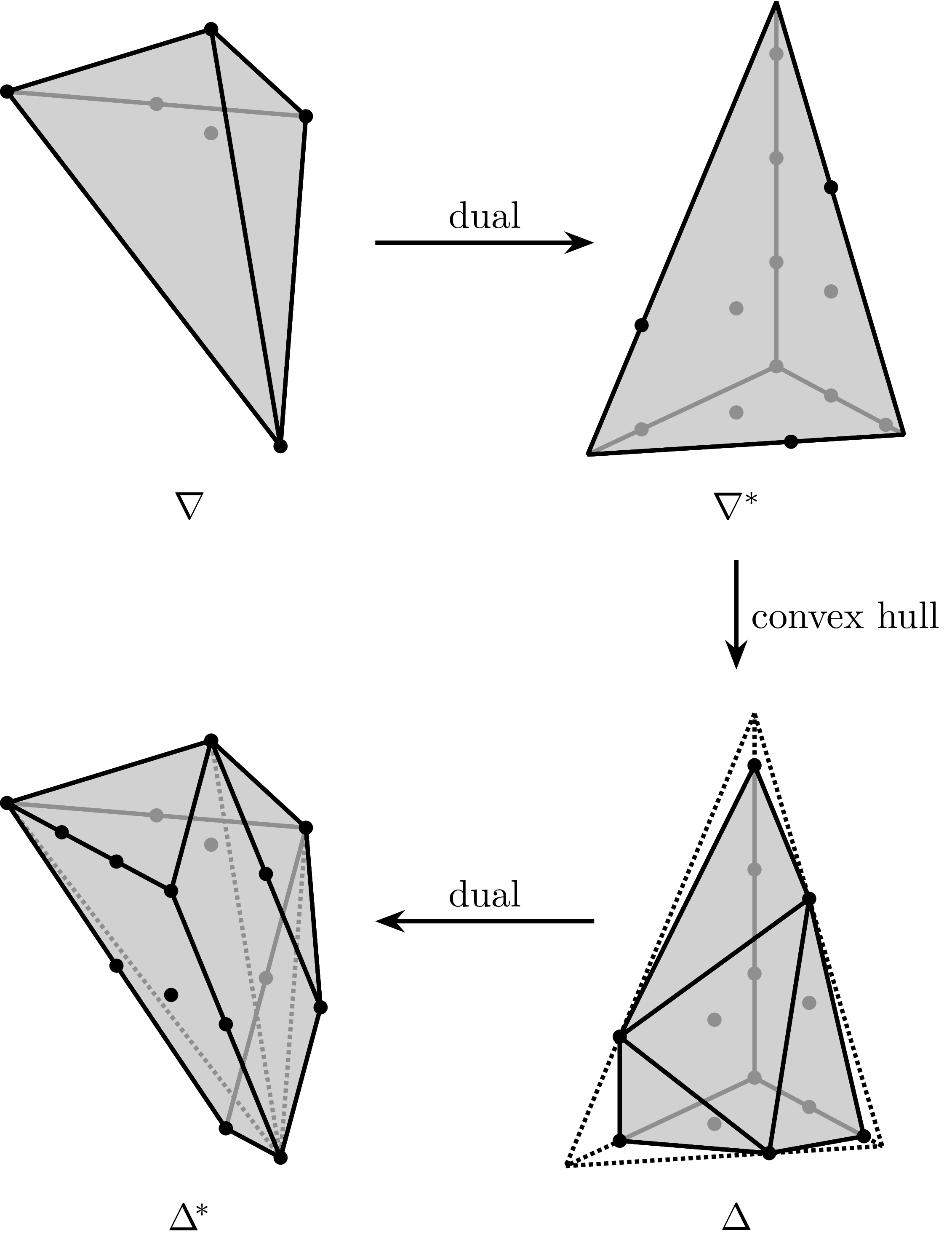
In higher dimensions, the situation becomes more complex. Not all IP polytopes are reflexive, and generally, .
This example shows the construction of the three-dimensional polytope with
weight system (2, 3, 4, 5) and its dual . Lattice points lying on the
polytopes are indicated by dots. has 7 vertices and 13 lattice points, also has 7 vertices, but 16 lattice points.
The counts of reflexive single-weight-system polytopes by dimension are:
| reflexive single-weight-system polytopes | |
|---|---|
| 2 | 3 |
| 3 | 95 |
| 4 | 184,026 |
| 5 | (this dataset) 185,269,499,015 |
One should note that distinct weight systems may well lead to the same polytope (we have not checked how often this occurs). In particular it seems that polytopes with a small number of lattice points are generated many times.