
File size: 39,183 Bytes
91b0698 20a07ea 91b0698 20a07ea 91b0698 20a07ea 91b0698 20a07ea 91b0698 20a07ea 91b0698 20a07ea 91b0698 20a07ea 91b0698 20a07ea 91b0698 20a07ea 91b0698 20a07ea 91b0698 20a07ea 91b0698 20a07ea 91b0698 20a07ea 91b0698 20a07ea 91b0698 20a07ea 91b0698 20a07ea 91b0698 20a07ea 91b0698 20a07ea 91b0698 20a07ea 91b0698 20a07ea 91b0698 20a07ea 91b0698 20a07ea 91b0698 20a07ea 91b0698 20a07ea 91b0698 20a07ea 91b0698 20a07ea 91b0698 20a07ea 91b0698 20a07ea 91b0698 20a07ea 91b0698 20a07ea 91b0698 20a07ea 91b0698 20a07ea 91b0698 20a07ea 91b0698 20a07ea 91b0698 20a07ea 91b0698 20a07ea 91b0698 20a07ea 91b0698 20a07ea 91b0698 20a07ea 91b0698 20a07ea 91b0698 20a07ea 91b0698 20a07ea 91b0698 20a07ea 91b0698 20a07ea 91b0698 20a07ea 91b0698 20a07ea 91b0698 20a07ea 91b0698 20a07ea 91b0698 20a07ea 91b0698 20a07ea 91b0698 20a07ea 91b0698 20a07ea 91b0698 20a07ea 91b0698 20a07ea 91b0698 20a07ea 91b0698 20a07ea 91b0698 20a07ea 91b0698 20a07ea 91b0698 20a07ea 91b0698 20a07ea 91b0698 20a07ea 91b0698 20a07ea 91b0698 20a07ea 91b0698 20a07ea 91b0698 20a07ea 91b0698 20a07ea 91b0698 20a07ea 91b0698 20a07ea 91b0698 20a07ea 91b0698 20a07ea 91b0698 20a07ea 91b0698 20a07ea 91b0698 20a07ea 91b0698 20a07ea 91b0698 20a07ea 91b0698 20a07ea 91b0698 20a07ea 91b0698 20a07ea 91b0698 20a07ea 91b0698 20a07ea 91b0698 20a07ea 91b0698 20a07ea 91b0698 20a07ea 91b0698 20a07ea 91b0698 20a07ea 91b0698 20a07ea 91b0698 20a07ea 91b0698 20a07ea 91b0698 20a07ea |
1 2 3 4 5 6 7 8 9 10 11 12 13 14 15 16 17 18 19 20 21 22 23 24 25 26 27 28 29 30 31 32 33 34 35 36 37 38 39 40 41 42 43 44 45 46 47 48 49 50 51 52 53 54 55 56 57 58 59 60 61 62 63 64 65 66 67 68 69 70 71 72 73 74 75 76 77 78 79 80 81 82 83 84 85 86 87 88 89 90 91 92 93 94 95 96 97 98 99 100 101 102 103 104 105 106 107 108 109 110 111 112 113 114 115 116 117 118 119 120 121 122 123 124 125 126 127 128 129 130 131 132 133 134 135 136 137 138 139 140 141 142 143 144 145 146 147 148 149 150 151 152 153 154 155 156 157 158 159 160 161 162 163 164 165 166 167 168 169 170 171 172 173 174 175 176 177 178 179 180 181 182 183 184 185 186 187 188 189 190 191 192 193 194 195 196 197 198 199 200 201 202 203 204 205 206 207 208 209 210 211 212 213 214 215 216 217 218 219 220 221 222 223 224 225 226 227 228 229 230 231 232 233 234 235 236 237 238 239 240 241 242 243 244 245 246 247 248 249 250 251 252 253 254 255 256 257 258 259 260 261 262 263 264 265 266 267 268 269 270 271 272 273 274 275 276 277 278 279 280 281 282 283 284 285 286 287 288 289 290 291 292 293 294 295 296 297 298 299 300 301 302 303 304 305 306 307 308 309 310 311 312 313 314 315 316 317 318 319 320 321 322 323 324 325 326 327 328 329 330 331 332 333 334 335 336 337 338 339 340 341 342 343 344 345 346 347 348 349 350 351 352 353 354 355 356 357 358 359 360 361 362 363 364 365 366 367 368 369 370 371 372 373 374 375 376 377 378 379 380 381 382 383 384 385 386 387 388 389 390 391 392 393 394 395 396 397 398 399 400 401 402 403 404 405 406 407 408 409 410 411 412 413 414 415 416 417 418 419 420 421 422 423 424 425 426 427 428 429 430 431 432 433 434 435 436 437 438 439 440 441 442 443 444 445 446 447 448 449 450 451 452 453 454 455 456 457 458 459 460 461 462 463 464 465 466 467 468 469 470 471 472 473 474 475 476 477 478 479 480 481 482 483 484 485 486 487 488 489 490 491 492 493 494 495 496 497 498 499 500 501 502 503 504 505 506 507 508 509 510 511 512 513 514 515 516 517 518 519 520 521 522 523 524 525 526 527 528 529 530 531 532 533 534 535 536 537 538 539 540 541 542 543 544 545 546 547 548 549 550 551 552 553 554 555 556 557 558 559 560 561 562 563 564 565 566 567 568 569 570 571 572 573 574 575 576 577 578 579 580 581 582 583 584 585 586 587 588 589 590 591 592 593 594 595 596 597 598 599 600 601 602 603 604 605 606 607 608 609 610 611 612 613 614 615 616 617 618 619 620 621 622 623 624 625 626 627 628 629 630 631 632 633 634 635 636 637 638 639 640 641 642 643 644 645 646 647 648 649 650 651 652 653 654 655 656 657 658 659 660 661 662 663 664 665 666 667 668 669 670 671 672 673 674 675 676 677 678 679 680 681 682 683 684 685 686 687 688 689 690 691 692 693 694 695 696 697 698 699 700 701 702 703 704 705 706 707 708 709 710 711 712 713 714 715 716 717 718 719 720 721 722 723 724 725 726 727 728 729 730 731 732 733 734 735 736 737 738 739 740 741 742 743 744 745 746 747 748 749 750 751 752 753 754 755 756 757 758 759 760 761 762 763 764 765 766 767 768 769 770 771 772 773 774 775 776 777 778 779 780 781 782 783 784 785 786 787 788 789 790 791 792 793 794 795 796 797 798 799 800 801 802 803 804 805 806 807 808 809 810 811 812 813 814 815 816 817 818 819 820 821 822 823 824 825 826 827 828 829 830 831 832 833 834 835 836 837 838 839 840 841 842 843 844 845 846 847 848 849 850 851 852 853 854 855 856 857 858 859 860 861 862 863 864 865 866 867 868 869 870 871 872 873 874 875 876 877 878 879 880 881 882 883 884 885 886 887 |
---
标题:“使用 🤗 Transformers 进行概率时间序列预测”
缩略图:/blog/assets/118_time-series-transformers/thumbnail.png
作者:
- 用户:nielsr
- 用户:kashif
---
<h1>使用 🤗 Transformers 进行概率时间序列预测</h1>
<!-- {blog_metadata} -->
<!-- {authors} -->
<script async="None" defer="None" src="https://unpkg.com/medium-zoom-element@0/dist/medium-zoom-element.min.js"></script>
<a target="_blank" href="https://colab.research.google.com/github/huggingface/notebooks/blob/main/examples/time-series-transformers.ipynb">
<img src="https://colab.research.google.com/assets/colab-badge.svg" alt="Open In Colab"></img>
</a>
## 介绍
时间序列预测是一个重要的科学和商业问题,因此最近通过使用[基于深度学习](https://dl.acm.org/doi/abs/10.1145/3533382) 而不是[经典方法](https://otexts.com/fpp3/)的模型也涌现出诸多创新。ARIMA 等经典方法与新颖的深度学习方法之间的一个重要区别如下。
- 关于基于深度学习进行时间序列预测的论文:
<url>https://dl.acm.org/doi/abs/10.1145/3533382</url>
- 《预测: 方法与实践》在线课本的中文版:
<url>https://otexts.com/fppcn/</url>
## 概率预测
通常,经典方法针对数据集中的每个时间序列单独拟合。这些通常被称为“单一”或“局部”方法。然而,当处理某些应用程序的大量时间序列时,在所有可用时间序列上训练一个“全局”模型是有益的,这使模型能够从许多不同的来源学习潜在的表示。
一些经典方法是点值的 (point-valued)(意思是每个时间步只输出一个值),并且通过最小化关于基本事实数据的 L2 或 L1 类型的损失来训练模型。然而,由于预测经常用于实际决策流程中,甚至在循环中有人的干预,让模型同时也提供预测的不确定性更加有益。这也称为“概率预测”,而不是“点预测”。这需要对可以采样的概率分布进行建模。
所以简而言之,我们希望训练**全局概率**模型,而不是训练局部点预测模型。深度学习非常适合这一点,因为神经网络可以从几个相关的时间序列中学习表示,并对数据的不确定性进行建模。
在概率设定中学习某些选定参数分布的未来参数很常见,例如高斯分布 (Gaussian) 或 Student-T,或者学习条件分位数函数 (conditional quantile function),或使用适应时间序列设置的共型预测 (Conformal Prediction) 框架。方法的选择不会影响到建模,因此通常可以将其视为另一个超参数。通过采用经验均值或中值,人们总是可以将概率模型转变为点预测模型。
## 时间序列 Transformer
正如人们所想象的那样,在对本来就连续的时间序列数据建模方面,研究人员提出了使用循环神经网络 (RNN) (如 LSTM 或 GRU) 或卷积网络 (CNN) 的模型,或利用最近兴起的基于 Transformer 的训练方法,都很自然地适合时间序列预测场景。
在这篇博文中,我们将利用传统 vanilla Transformer [(参考 Vaswani 等 2017 年发表的论文)](https://arxiv.org/abs/1706.03762) 进行**单变量**概率预测 (univariate probabilistic forecasting) 任务 (即预测每个时间序列的一维分布) 。 由于 Encoder-Decoder Transformer 很好地封装了几个归纳偏差,所以它成为了我们预测的自然选择。
- 传统 vanilla Transformer 论文链接:
<url>https://arxiv.org/abs/1706.03762</url>
首先,使用 Encoder-Decoder 架构在推理时很有帮助。通常对于一些记录的数据,我们希望提前预知未来的一些预测步骤。可以认为这个过程类似于文本生成任务,即给定上下文,采样下一个词元 (token) 并将其传回解码器 (也称为“自回归生成”) 。类似地,我们也可以在给定某种分布类型的情况下,从中抽样以提供预测,直到我们期望的预测范围。这被称为贪婪采样 (Greedy Sampling)/搜索,[此处](https://huggingface.co/blog/how-to-generate) 有一篇关于 NLP 场景预测的精彩博文。
<url>https://hf.co/blog/how-to-generate</url>
其次,Transformer 帮助我们训练可能包含成千上万个时间点的时间序列数据。由于注意力机制的时间和内存限制,一次性将 **所有** 时间序列的完整历史输入模型或许不太可行。因此,在为随机梯度下降 (SGD) 构建批次时,可以考虑适当的上下文窗口大小,并从训练数据中对该窗口和后续预测长度大小的窗口进行采样。可以将调整过大小的上下文窗口传递给编码器、预测窗口传递给 **causal-masked** 解码器。这样一来,解码器在学习下一个值时只能查看之前的时间步。这相当于人们训练用于机器翻译的 vanilla Transformer 的过程,称为“教师强制 (Teacher Forcing)”。
Transformers 相对于其他架构的另一个好处是,我们可以将缺失值 (这在时间序列场景中很常见) 作为编码器或解码器的额外掩蔽值 (mask),并且仍然可以在不诉诸于填充或插补的情况下进行训练。这相当于 Transformers 库中 BERT 和 GPT-2 等模型的 `attention_mask`,在注意力矩阵 (attention matrix) 的计算中不包括填充词元。
由于传统 vanilla Transformer 的平方运算和内存要求,Transformer 架构的一个缺点是上下文和预测窗口的大小受到限制。关于这一点,可以参阅 [Tay 等人于 2020 年发表的调研报告](https://arxiv.org/abs/2009.06732) 。此外,由于 Transformer 是一种强大的架构,与 [其他方法](https://openreview.net/pdf?id=D7YBmfX_VQy) 相比,它可能会过拟合或更容易学习虚假相关性。
- Tay 等 2020 年发表的调研报告地址:
<url>https://arxiv.org/abs/2009.06732</url>
- 上述关于其他预测时间线方法的论文地址:
<url>https://openreview.net/pdf?id=D7YBmfX_VQy</url>
🤗 Transformers 库带有一个普通的概率时间序列 Transformer 模型,简称为 [Time Series Transformer](https://huggingface.co/docs/transformers/model_doc/time_series_transformer)。在这篇文章后面的内容中,我们将展示如何在自定义数据集上训练此类模型。
Time Series Transformer 模型文档:
<url>https://hf.co/docs/transformers/model_doc/time_series_transformer</url>
## 设置环境
首先,让我们安装必要的库: 🤗 Transformers、🤗 Datasets、🤗 Evaluate、🤗 Accelerate 和 [GluonTS](https://github.com/awslabs/gluonts)。
GluonTS 的 GitHub 仓库:
<url>https://github.com/awslabs/gluonts</url>
正如我们将展示的那样,GluonTS 将用于转换数据以创建特征以及创建适当的训练、验证和测试批次。
```python
!pip install -q transformers
!pip install -q datasets
!pip install -q evaluate
!pip install -q accelerate
!pip install -q gluonts ujson
```
## 加载数据集
在这篇博文中,我们将使用 [Hugging Face Hub](https://huggingface.co/datasets/monash_tsf) 上提供的 `tourism_monthly` 数据集。该数据集包含澳大利亚 366 个地区的每月旅游流量。
`tourism_monthly` 数据集地址:
<url>https://hf.co/datasets/monash_tsf</url>
此数据集是 [Monash Time Series Forecasting](https://forecastingdata.org/) 存储库的一部分,该存储库收纳了是来自多个领域的时间序列数据集。它可以看作是时间序列预测的 GLUE 基准。
Monash Time Series Forecasting 存储库链接:
<url>https://forecastingdata.org/</url>
```python
from datasets import load_dataset
dataset = load_dataset("monash_tsf", "tourism_monthly")
```
可以看出,数据集包含 3 个片段: 训练、验证和测试。
```python
dataset
>>> DatasetDict({
train: Dataset({
features: ['start', 'target', 'feat_static_cat', 'feat_dynamic_real', 'item_id'],
num_rows: 366
})
test: Dataset({
features: ['start', 'target', 'feat_static_cat', 'feat_dynamic_real', 'item_id'],
num_rows: 366
})
validation: Dataset({
features: ['start', 'target', 'feat_static_cat', 'feat_dynamic_real', 'item_id'],
num_rows: 366
})
})
```
每个示例都包含一些键,其中 `start` 和 `target` 是最重要的键。让我们看一下数据集中的第一个时间序列:
```python
train_example = dataset['train'][0]
train_example.keys()
>>> dict_keys(['start', 'target', 'feat_static_cat', 'feat_dynamic_real', 'item_id'])
```
`start` 仅指示时间序列的开始 (类型为 `datetime`) ,而 `target` 包含时间序列的实际值。
`start` 将有助于将时间相关的特征添加到时间序列值中,作为模型的额外输入 (例如“一年中的月份”) 。因为我们已经知道数据的频率是 `每月`,所以也能推算第二个值的时间戳为 `1979-02-01`,等等。
```python
print(train_example['start'])
print(train_example['target'])
>>> 1979-01-01 00:00:00
[1149.8699951171875, 1053.8001708984375, ..., 5772.876953125]
```
验证集包含与训练集相同的数据,只是数据时间范围延长了 `prediction_length` 那么多。这使我们能够根据真实情况验证模型的预测。
与验证集相比,测试集还是比验证集多包含 `prediction_length` 时间的数据 (或者使用比训练集多出数个 `prediction_length` 时长数据的测试集,实现在多重滚动窗口上的测试任务)。
```python
validation_example = dataset['validation'][0]
validation_example.keys()
>>> dict_keys(['start', 'target', 'feat_static_cat', 'feat_dynamic_real', 'item_id'])
```
验证的初始值与相应的训练示例完全相同:
```python
print(validation_example['start'])
print(validation_example['target'])
>>> 1979-01-01 00:00:00
[1149.8699951171875, 1053.8001708984375, ..., 5985.830078125]
```
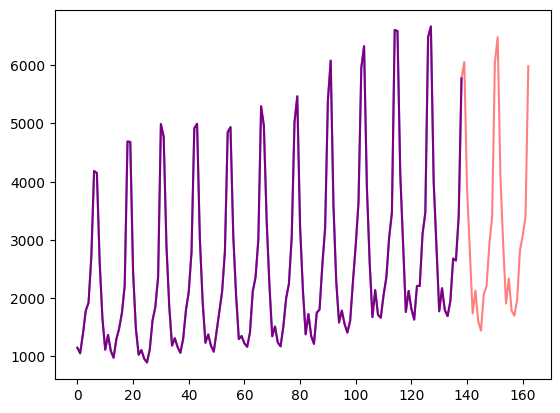
但是,与训练示例相比,此示例具有 `prediction_length=24` 个额外的数据。让我们验证一下。
```python
freq = "1M"
prediction_length = 24
assert len(train_example['target']) + prediction_length == len(validation_example['target'])
```
让我们可视化一下:
```python
import matplotlib.pyplot as plt
figure, axes = plt.subplots()
axes.plot(train_example['target'], color="blue")
axes.plot(validation_example['target'], color="red", alpha=0.5)
plt.show()
```
下面拆分数据:
```python
train_dataset = dataset["train"]
test_dataset = dataset["test"]
```
## 将 `start` 更新为 `pd.Period`
我们要做的第一件事是根据数据的 `freq` 值将每个时间序列的 `start` 特征转换为 pandas 的 `Period` 索引:
```python
from functools import lru_cache
import pandas as pd
import numpy as np
@lru_cache(10_000)
def convert_to_pandas_period(date, freq):
return pd.Period(date, freq)
def transform_start_field(batch, freq):
batch["start"] = [convert_to_pandas_period(date, freq) for date in batch["start"]]
return batch
```
这里我们使用 `datasets` 的 [`set_transform`](https://huggingface.co/docs/datasets/v2.7.0/en/package_reference/main_classes#datasets.Dataset.set_transform) 来实现:
`set_transform` 文档地址:
<url>https://hf.co/docs/datasets/v2.7.0/en/package_reference/main_classes</url>
```python
from functools import partial
train_dataset.set_transform(partial(transform_start_field, freq=freq))
test_dataset.set_transform(partial(transform_start_field, freq=freq))
```
## 定义模型
接下来,让我们实例化一个模型。该模型将从头开始训练,因此我们不使用 `from_pretrained` 方法,而是从 [`config`](https://huggingface.co/docs/transformers/model_doc/time_series_transformer#transformers.TimeSeriesTransformerConfig) 中随机初始化模型。
我们为模型指定了几个附加参数:
- `prediction_length` (在我们的例子中是 `24` 个月) : 这是 Transformer 的解码器将学习预测的范围;
- `context_length`: 如果未指定 `context_length`,模型会将 `context_length` (编码器的输入) 设置为等于 `prediction_length`;
- 给定频率的 `lags`(滞后): 这将决定模型“回头看”的程度,也会作为附加特征。例如对于 `Daily` 频率,我们可能会考虑回顾 `[1, 2, 7, 30, ...]`,也就是回顾 1、2……天的数据,而对于 Minute` 数据,我们可能会考虑 `[1, 30, 60, 60*24, ...]` 等;
- 时间特征的数量: 在我们的例子中设置为 `2`,因为我们将添加 `MonthOfYear` 和 `Age` 特征;
- 静态类别型特征的数量: 在我们的例子中,这将只是 `1`,因为我们将添加一个“时间序列 ID”特征;
- 基数: 将每个静态类别型特征的值的数量构成一个列表,对于本例来说将是 `[366]`,因为我们有 366 个不同的时间序列;
- 嵌入维度: 每个静态类别型特征的嵌入维度,也是构成列表。例如 `[3]` 意味着模型将为每个 ``366` 时间序列 (区域) 学习大小为 `3` 的嵌入向量。
让我们使用 GluonTS 为给定频率 (“每月”) 提供的默认滞后值:
```python
from gluonts.time_feature import get_lags_for_frequency
lags_sequence = get_lags_for_frequency(freq)
print(lags_sequence)
>>> [1, 2, 3, 4, 5, 6, 7, 11, 12, 13, 23, 24, 25, 35, 36, 37]
```
这意味着我们每个时间步将回顾长达 37 个月的数据,作为附加特征。
我们还检查 GluonTS 为我们提供的默认时间特征:
```python
from gluonts.time_feature import time_features_from_frequency_str
time_features = time_features_from_frequency_str(freq)
print(time_features)
>>> [<function month_of_year at 0x7fa496d0ca70>]
```
在这种情况下,只有一个特征,即“一年中的月份”。这意味着对于每个时间步长,我们将添加月份作为标量值 (例如,如果时间戳为 "january",则为 `1`;如果时间戳为 "february",则为 `2`,等等) 。
我们现在准备好定义模型需要的所有内容了:
```python
from transformers import TimeSeriesTransformerConfig, TimeSeriesTransformerForPrediction
config = TimeSeriesTransformerConfig(
prediction_length=prediction_length,
context_length=prediction_length*3, # context length
lags_sequence=lags_sequence,
num_time_features=len(time_features) + 1, # we'll add 2 time features ("month of year" and "age", see further)
num_static_categorical_features=1, # we have a single static categorical feature, namely time series ID
cardinality=[len(train_dataset)], # it has 366 possible values
embedding_dimension=[2], # the model will learn an embedding of size 2 for each of the 366 possible values
encoder_layers=4,
decoder_layers=4,
)
model = TimeSeriesTransformerForPrediction(config)
```
请注意,与 🤗 Transformers 库中的其他模型类似,[`TimeSeriesTransformerModel`](https://huggingface.co/docs/transformers/model_doc/time_series_transformer#transformers.TimeSeriesTransformerModel) 对应于没有任何顶部前置头的编码器-解码器 Transformer,而 [`TimeSeriesTransformerForPrediction`](https://huggingface.co/docs/transformers/model_doc/time_series_transformer#transformers.TimeSeriesTransformerForPrediction) 对应于顶部有一个分布前置头 (**distribution head**) 的 `TimeSeriesTransformerModel`。默认情况下,该模型使用 Student-t 分布 (也可以自行配置):
上述两个模型的文档链接:
<url>https://hf.co/docs/transformers/model_doc/time_series_transformer</url>
```python
model.config.distribution_output
>>> student_t
```
这是具体实现层面与用于 NLP 的 Transformers 的一个重要区别,其中头部通常由一个固定的分类分布组成,实现为 `nn.Linear` 层。
## 定义转换
接下来,我们定义数据的转换,尤其是需要基于样本数据集或通用数据集来创建其中的时间特征。
同样,我们用到了 GluonTS 库。这里定义了一个 `Chain` (有点类似于图像训练的 `torchvision.transforms.Compose`) 。它允许我们将多个转换组合到一个流水线中。
```python
from gluonts.time_feature import time_features_from_frequency_str, TimeFeature, get_lags_for_frequency
from gluonts.dataset.field_names import FieldName
from gluonts.transform import (
AddAgeFeature,
AddObservedValuesIndicator,
AddTimeFeatures,
AsNumpyArray,
Chain,
ExpectedNumInstanceSampler,
InstanceSplitter,
RemoveFields,
SelectFields,
SetField,
TestSplitSampler,
Transformation,
ValidationSplitSampler,
VstackFeatures,
RenameFields,
)
```
下面的转换代码带有注释供大家查看具体的操作步骤。从全局来说,我们将迭代数据集的各个时间序列并添加、删除某些字段或特征:
```python
from transformers import PretrainedConfig
def create_transformation(freq: str, config: PretrainedConfig) -> Transformation:
remove_field_names = []
if config.num_static_real_features == 0:
remove_field_names.append(FieldName.FEAT_STATIC_REAL)
if config.num_dynamic_real_features == 0:
remove_field_names.append(FieldName.FEAT_DYNAMIC_REAL)
# 类似 torchvision.transforms.Compose
return Chain(
# 步骤 1: 如果静态或动态字段没有特殊声明,则将它们移除
[RemoveFields(field_names=remove_field_names)]
# 步骤 2: 如果静态特征存在,就直接使用,否则添加一些虚拟值
+ (
[SetField(output_field=FieldName.FEAT_STATIC_CAT, value=[0])]
if not config.num_static_categorical_features > 0
else []
)
+ (
[SetField(output_field=FieldName.FEAT_STATIC_REAL, value=[0.0])]
if not config.num_static_real_features > 0
else []
)
# 步骤 3: 将数据转换为 NumPy 格式 (应该用不上)
+ [
AsNumpyArray(
field=FieldName.FEAT_STATIC_CAT,
expected_ndim=1,
dtype=int,
),
AsNumpyArray(
field=FieldName.FEAT_STATIC_REAL,
expected_ndim=1,
),
AsNumpyArray(
field=FieldName.TARGET,
# 接下来一行我们为时间维度的数据加上 1
expected_ndim=1 if config.input_size==1 else 2,
),
# 步骤 4: 目标值遇到 NaN 时,用 0 填充
# 然后返回观察值的掩蔽值
# 存在观察值时为 true,NaN 时为 false
# 解码器会使用这些掩蔽值 (遇到非观察值时不会产生损失值)
# 具体可以查看 xxxForPrediction 模型的 loss_weights 说明
AddObservedValuesIndicator(
target_field=FieldName.TARGET,
output_field=FieldName.OBSERVED_VALUES,
),
# 步骤 5: 根据数据集的 freq 字段添加暂存值
# 也就是这里的“一年中的月份”
# 这些暂存值将作为定位编码使用
AddTimeFeatures(
start_field=FieldName.START,
target_field=FieldName.TARGET,
output_field=FieldName.FEAT_TIME,
time_features=time_features_from_frequency_str(freq),
pred_length=config.prediction_length,
),
# 步骤 6: 添加另一个暂存值 (一个单一数字)
# 用于让模型知道当前值在时间序列中的位置
# 类似于一个步进计数器
AddAgeFeature(
target_field=FieldName.TARGET,
output_field=FieldName.FEAT_AGE,
pred_length=config.prediction_length,
log_scale=True,
),
# 步骤 7: 将所有暂存特征值纵向堆叠
VstackFeatures(
output_field=FieldName.FEAT_TIME,
input_fields=[FieldName.FEAT_TIME, FieldName.FEAT_AGE]
+ ([FieldName.FEAT_DYNAMIC_REAL] if config.num_dynamic_real_features > 0 else []),
),
# 步骤 8: 建立字段名和 Hugging Face 惯用字段名之间的映射
RenameFields(
mapping={
FieldName.FEAT_STATIC_CAT: "static_categorical_features",
FieldName.FEAT_STATIC_REAL: "static_real_features",
FieldName.FEAT_TIME: "time_features",
FieldName.TARGET: "values",
FieldName.OBSERVED_VALUES: "observed_mask",
}
),
]
)
```
## 定义 `InstanceSplitter`
对于训练、验证、测试步骤,接下来我们创建一个 `InstanceSplitter`,用于从数据集中对窗口进行采样 (因为由于时间和内存限制,我们无法将整个历史值传递给 Transformer)。
实例拆分器从数据中随机采样大小为 `context_length` 和后续大小为 `prediction_length` 的窗口,并将 `past_` 或 `future_` 键附加到各个窗口的任何临时键。这确保了 `values` 被拆分为 `past_values` 和后续的 `future_values` 键,它们将分别用作编码器和解码器的输入。同样我们还需要修改 `time_series_fields` 参数中的所有键:
```python
from gluonts.transform.sampler import InstanceSampler
from typing import Optional
def create_instance_splitter(config: PretrainedConfig, mode: str, train_sampler: Optional[InstanceSampler] = None,
validation_sampler: Optional[InstanceSampler] = None,) -> Transformation:
assert mode in ["train", "validation", "test"]
instance_sampler = {
"train": train_sampler or ExpectedNumInstanceSampler(
num_instances=1.0, min_future=config.prediction_length
),
"validation": validation_sampler or ValidationSplitSampler(
min_future=config.prediction_length
),
"test": TestSplitSampler(),
}[mode]
return InstanceSplitter(
target_field="values",
is_pad_field=FieldName.IS_PAD,
start_field=FieldName.START,
forecast_start_field=FieldName.FORECAST_START,
instance_sampler=instance_sampler,
past_length=config.context_length + max(config.lags_sequence),
future_length=config.prediction_length,
time_series_fields=[
"time_features",
"observed_mask",
],
)
```
## 创建 PyTorch 数据加载器
有了数据,下一步需要创建 PyTorch DataLoaders。它允许我们批量处理成对的 (输入, 输出) 数据,即 (`past_values` , `future_values`)。
```python
from gluonts.itertools import Cyclic, IterableSlice, PseudoShuffled
from gluonts.torch.util import IterableDataset
from torch.utils.data import DataLoader
from typing import Iterable
def create_train_dataloader(
config: PretrainedConfig,
freq,
data,
batch_size: int,
num_batches_per_epoch: int,
shuffle_buffer_length: Optional[int] = None,
**kwargs,
) -> Iterable:
PREDICTION_INPUT_NAMES = [
"static_categorical_features",
"static_real_features",
"past_time_features",
"past_values",
"past_observed_mask",
"future_time_features",
]
TRAINING_INPUT_NAMES = PREDICTION_INPUT_NAMES + [
"future_values",
"future_observed_mask",
]
transformation = create_transformation(freq, config)
transformed_data = transformation.apply(data, is_train=True)
# we initialize a Training instance
instance_splitter = create_instance_splitter(
config, "train"
) + SelectFields(TRAINING_INPUT_NAMES)
# the instance splitter will sample a window of
# context length + lags + prediction length (from the 366 possible transformed time series)
# randomly from within the target time series and return an iterator.
training_instances = instance_splitter.apply(
Cyclic(transformed_data)
if shuffle_buffer_length is None
else PseudoShuffled(
Cyclic(transformed_data),
shuffle_buffer_length=shuffle_buffer_length,
)
)
# from the training instances iterator we now return a Dataloader which will
# continue to sample random windows for as long as it is called
# to return batch_size of the appropriate tensors ready for training!
return IterableSlice(
iter(
DataLoader(
IterableDataset(training_instances),
batch_size=batch_size,
**kwargs,
)
),
num_batches_per_epoch,
)
```
```python
def create_test_dataloader(
config: PretrainedConfig,
freq,
data,
batch_size: int,
**kwargs,
):
PREDICTION_INPUT_NAMES = [
"static_categorical_features",
"static_real_features",
"past_time_features",
"past_values",
"past_observed_mask",
"future_time_features",
]
transformation = create_transformation(freq, config)
transformed_data = transformation.apply(data, is_train=False)
# we create a Test Instance splitter which will sample the very last
# context window seen during training only for the encoder.
instance_splitter = create_instance_splitter(
config, "test"
) + SelectFields(PREDICTION_INPUT_NAMES)
# we apply the transformations in test mode
testing_instances = instance_splitter.apply(transformed_data, is_train=False)
# This returns a Dataloader which will go over the dataset once.
return DataLoader(IterableDataset(testing_instances), batch_size=batch_size, **kwargs)
```
```python
train_dataloader = create_train_dataloader(
config=config,
freq=freq,
data=train_dataset,
batch_size=256,
num_batches_per_epoch=100,
)
test_dataloader = create_test_dataloader(
config=config,
freq=freq,
data=test_dataset,
batch_size=64,
)
```
让我们检查第一批:
```python
batch = next(iter(train_dataloader))
for k,v in batch.items():
print(k,v.shape, v.type())
>>> static_categorical_features torch.Size([256, 1]) torch.LongTensor
static_real_features torch.Size([256, 1]) torch.FloatTensor
past_time_features torch.Size([256, 181, 2]) torch.FloatTensor
past_values torch.Size([256, 181]) torch.FloatTensor
past_observed_mask torch.Size([256, 181]) torch.FloatTensor
future_time_features torch.Size([256, 24, 2]) torch.FloatTensor
future_values torch.Size([256, 24]) torch.FloatTensor
future_observed_mask torch.Size([256, 24]) torch.FloatTensor
```
可以看出,我们没有将 `input_ids` 和 `attention_mask` 提供给编码器 (训练 NLP 模型时也是这种情况),而是提供 `past_values`,以及 `past_observed_mask`、`past_time_features`、`static_categorical_features` 和 `static_real_features` 几项数据。
解码器的输入包括 `future_values`、`future_observed_mask` 和 `future_time_features`。 `future_values` 可以看作等同于 NLP 训练中的 `decoder_input_ids`。
我们可以参考 [Time Series Transformer 文档](https://huggingface.co/docs/transformers/model_doc/time_series_transformer#transformers.TimeSeriesTransformerForPrediction.forward.past_values) 以获得对它们中每一个的详细解释。
## 前向传播
让我们对刚刚创建的批次执行一次前向传播:
```python
# perform forward pass
outputs = model(
past_values=batch["past_values"],
past_time_features=batch["past_time_features"],
past_observed_mask=batch["past_observed_mask"],
static_categorical_features=batch["static_categorical_features"],
static_real_features=batch["static_real_features"],
future_values=batch["future_values"],
future_time_features=batch["future_time_features"],
future_observed_mask=batch["future_observed_mask"],
output_hidden_states=True
)
```
```python
print("Loss:", outputs.loss.item())
>>> Loss: 9.141253471374512
```
目前,该模型返回了损失值。这是由于解码器会自动将 `future_values` 向右移动一个位置以获得标签。这允许计算预测结果和标签值之间的误差。
另请注意,解码器使用 Causal Mask 来避免预测未来,因为它需要预测的值在 `future_values` 张量中。
## 训练模型
是时候训练模型了!我们将使用标准的 PyTorch 训练循环。
这里我们用到了 🤗 [Accelerate](https://huggingface.co/docs/accelerate/index) 库,它会自动将模型、优化器和数据加载器放置在适当的 `device` 上。
🤗 Accelerate 文档地址:
<url>https://hf.co/docs/accelerate/index</url>
```python
from accelerate import Accelerator
from torch.optim import Adam
accelerator = Accelerator()
device = accelerator.device
model.to(device)
optimizer = Adam(model.parameters(), lr=1e-3)
model, optimizer, train_dataloader = accelerator.prepare(
model, optimizer, train_dataloader,
)
for epoch in range(40):
model.train()
for batch in train_dataloader:
optimizer.zero_grad()
outputs = model(
static_categorical_features=batch["static_categorical_features"].to(device),
static_real_features=batch["static_real_features"].to(device),
past_time_features=batch["past_time_features"].to(device),
past_values=batch["past_values"].to(device),
future_time_features=batch["future_time_features"].to(device),
future_values=batch["future_values"].to(device),
past_observed_mask=batch["past_observed_mask"].to(device),
future_observed_mask=batch["future_observed_mask"].to(device),
)
loss = outputs.loss
# Backpropagation
accelerator.backward(loss)
optimizer.step()
print(loss.item())
```
## 推理
在推理时,建议使用 `generate()` 方法进行自回归生成,类似于 NLP 模型。
预测的过程会从测试实例采样器中获得数据。采样器会将数据集的每个时间序列的最后 `context_length` 那么长时间的数据采样出来,然后输入模型。请注意,这里需要把提前已知的 `future_time_features` 传递给解码器。
该模型将从预测分布中自回归采样一定数量的值,并将它们传回解码器最终得到预测输出:
```python
model.eval()
forecasts = []
for batch in test_dataloader:
outputs = model.generate(
static_categorical_features=batch["static_categorical_features"].to(device),
static_real_features=batch["static_real_features"].to(device),
past_time_features=batch["past_time_features"].to(device),
past_values=batch["past_values"].to(device),
future_time_features=batch["future_time_features"].to(device),
past_observed_mask=batch["past_observed_mask"].to(device),
)
forecasts.append(outputs.sequences.cpu().numpy())
```
该模型输出一个表示结构的张量 (`batch_size`, `number of samples`, `prediction length`)。
下面的输出说明: 对于大小为 64 的批次中的每个示例,我们将获得接下来 24 个月内的 100 个可能的值:
```python
forecasts[0].shape
>>> (64, 100, 24)
```
我们将垂直堆叠它们,以获得测试数据集中所有时间序列的预测:
```python
forecasts = np.vstack(forecasts)
print(forecasts.shape)
>>> (366, 100, 24)
```
我们可以根据测试集中存在的样本值,根据真实情况评估生成的预测。这里我们使用数据集中的每个时间序列的 [MASE](https://huggingface.co/spaces/evaluate-metric/mase) 和 [sMAPE](https://hf.co/spaces/evaluate-metric/smape) 指标 (metrics) 来评估:
- MASE 文档地址:
<url>https://hf.co/spaces/evaluate-metric/mase</url>
- sMAPE 文档地址:
<url>https://hf.co/spaces/evaluate-metric/smape</url>
```python
from evaluate import load
from gluonts.time_feature import get_seasonality
mase_metric = load("evaluate-metric/mase")
smape_metric = load("evaluate-metric/smape")
forecast_median = np.median(forecasts, 1)
mase_metrics = []
smape_metrics = []
for item_id, ts in enumerate(test_dataset):
training_data = ts["target"][:-prediction_length]
ground_truth = ts["target"][-prediction_length:]
mase = mase_metric.compute(
predictions=forecast_median[item_id],
references=np.array(ground_truth),
training=np.array(training_data),
periodicity=get_seasonality(freq))
mase_metrics.append(mase["mase"])
smape = smape_metric.compute(
predictions=forecast_median[item_id],
references=np.array(ground_truth),
)
smape_metrics.append(smape["smape"])
```
```python
print(f"MASE: {np.mean(mase_metrics)}")
>>> MASE: 1.361636922541396
print(f"sMAPE: {np.mean(smape_metrics)}")
>>> sMAPE: 0.17457818831512306
```
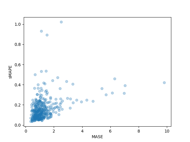
我们还可以单独绘制数据集中每个时间序列的结果指标,并观察到其中少数时间序列对最终测试指标的影响很大:
```python
plt.scatter(mase_metrics, smape_metrics, alpha=0.3)
plt.xlabel("MASE")
plt.ylabel("sMAPE")
plt.show()
```
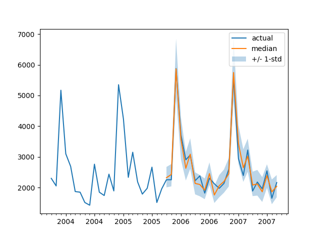
为了根据基本事实测试数据绘制任何时间序列的预测,我们定义了以下辅助绘图函数:
```python
import matplotlib.dates as mdates
def plot(ts_index):
fig, ax = plt.subplots()
index = pd.period_range(
start=test_dataset[ts_index][FieldName.START],
periods=len(test_dataset[ts_index][FieldName.TARGET]),
freq=freq,
).to_timestamp()
# Major ticks every half year, minor ticks every month,
ax.xaxis.set_major_locator(mdates.MonthLocator(bymonth=(1, 7)))
ax.xaxis.set_minor_locator(mdates.MonthLocator())
ax.plot(
index[-2*prediction_length:],
test_dataset[ts_index]["target"][-2*prediction_length:],
label="actual",
)
plt.plot(
index[-prediction_length:],
np.median(forecasts[ts_index], axis=0),
label="median",
)
plt.fill_between(
index[-prediction_length:],
forecasts[ts_index].mean(0) - forecasts[ts_index].std(axis=0),
forecasts[ts_index].mean(0) + forecasts[ts_index].std(axis=0),
alpha=0.3,
interpolate=True,
label="+/- 1-std",
)
plt.legend()
plt.show()
```
例如:
```python
plot(334)
```
我们如何与其他模型进行比较? [Monash Time Series Repository](https://forecastingdata.org/#results) 有一个测试集 MASE 指标的比较表。我们可以将自己的结果添加到其中作比较:
|Dataset | SES| Theta | TBATS| ETS | (DHR-)ARIMA| PR| CatBoost | FFNN | DeepAR | N-BEATS | WaveNet| **Transformer** (Our) |
|:------------------:|:-----------------:|:--:|:--:|:--:|:--:|:--:|:--:|:---:|:---:|:--:|:--:|:--:|
|Tourism Monthly | 3.306 | 1.649 | 1.751 | 1.526| 1.589| 1.678 |1.699| 1.582 | 1.409 | 1.574| 1.482 | **1.361**|
请注意,我们的模型击败了所有已知的其他模型 (另请参见相应 [论文](https://openreview.net/pdf?id=wEc1mgAjU-) 中的表 2) ,并且我们没有做任何超参数优化。我们仅仅花了 40 个完整训练调参周期来训练 Transformer。
上文对于此数据集的预测方法论文:
<url>https://openreview.net/pdf?id=wEc1mgAjU-</url>
当然,我们应该谦虚。从历史发展的角度来看,现在认为神经网络解决时间序列预测问题是正途,就好比当年的论文得出了 [“你需要的就是 XGBoost”](https://www.sciencedirect.com/science/article/pii/S0169207021001679) 的结论。我们只是很好奇,想看看神经网络能带我们走多远,以及 Transformer 是否会在这个领域发挥作用。这个特定的数据集似乎表明它绝对值得探索。
得出“你需要的就是 XGBoost”结论的论文地址:
<url>https://www.sciencedirect.com/science/article/pii/S0169207021001679</url>
## 下一步
我们鼓励读者尝试我们的 [Jupyter Notebook](https://colab.research.google.com/github/huggingface/notebooks/blob/main/examples/time-series-transformers.ipynb) 和来自 [Hugging Face Hub](https://huggingface.co/datasets/monash_tsf) 的其他时间序列数据集,并替换适当的频率和预测长度参数。对于您的数据集,需要将它们转换为 GluonTS 的惯用格式,在他们的 [文档](https://ts.gluon.ai/stable/tutorials/forecasting/extended_tutorial.html#What-is-in-a-dataset?) 里有非常清晰的说明。我们还准备了一个示例 [Notebook](https://github.com/huggingface/notebooks/blob/main/examples/time_series_datasets.ipynb),向您展示如何将数据集转换为 🤗 Hugging Face 数据集格式。
- Time Series Transformers Notebook:
<url>https://colab.research.google.com/github/huggingface/notebooks/blob/main/examples/time-series-transformers.ipynb</url>
- Hub 中的 Monash Time Series 数据集:
<url>https://hf.co/datasets/monash_tsf</url>
- GluonTS 阐述数据集格式的文档:
<url>https://ts.gluon.ai/stable/tutorials/forecasting/extended_tutorial.html</url>
- 演示数据集格式转换的 Notebook:
<url>https://github.com/huggingface/notebooks/blob/main/examples/time_series_datasets.ipynb</url>
正如时间序列研究人员所知,人们对“将基于 Transformer 的模型应用于时间序列”问题很感兴趣。传统 vanilla Transformer 只是众多基于注意力 (Attention) 的模型之一,因此需要向库中补充更多模型。
目前没有什么能妨碍我们继续探索对多变量时间序列 (multivariate time series) 进行建模,但是为此需要使用多变量分布头 (multivariate distribution head) 来实例化模型。目前已经支持了对角独立分布 (diagonal independent distributions),后续会增加其他多元分布支持。请继续关注未来的博客文章以及其中的教程。
路线图上的另一件事是时间序列分类。这需要将带有分类头的时间序列模型添加到库中,例如用于异常检测这类任务。
当前的模型会假设日期时间和时间序列值都存在,但在现实中这可能不能完全满足。例如 [WOODS](https://woods-benchmarks.github.io/) 给出的神经科学数据集。因此,我们还需要对当前模型进行泛化,使某些输入在整个流水线中可选。
WOODS 主页:
<url>https://woods-benchmarks.github.io/</url>
最后,NLP/CV 领域从[大型预训练模型](https://arxiv.org/abs/1810.04805) 中获益匪浅,但据我们所知,时间序列领域并非如此。基于 Transformer 的模型似乎是这一研究方向的必然之选,我们迫不及待地想看看研究人员和从业者会发现哪些突破!
大型预训练模型论文地址:
<url>https://arxiv.org/abs/1810.04805</url>
---
>>>> 英文原文: [Probabilistic Time Series Forecasting with 🤗 Transformers](https://huggingface.co/blog/time-series-transformers)
>>>>
>>>> 译者、排版: zhongdongy (阿东)
|