使用 🤗 Transformers 进行概率时间序列预测


介绍
时间序列预测是一个重要的科学和商业问题,因此最近通过使用 基于深度学习 而不是 经典方法 的模型也涌现出诸多创新。ARIMA 等经典方法与新颖的深度学习方法之间的一个重要区别如下。
概率预测
通常,经典方法针对数据集中的每个时间序列单独拟合。这些通常被称为“单一”或“局部”方法。然而,当处理某些应用程序的大量时间序列时,在所有可用时间序列上训练一个“全局”模型是有益的,这使模型能够从许多不同的来源学习潜在的表示。
一些经典方法是点值的 (point-valued)(意思是每个时间步只输出一个值),并且通过最小化关于基本事实数据的 L2 或 L1 类型的损失来训练模型。然而,由于预测经常用于实际决策流程中,甚至在循环中有人的干预,让模型同时也提供预测的不确定性更加有益。这也称为“概率预测”,而不是“点预测”。这需要对可以采样的概率分布进行建模。
所以简而言之,我们希望训练 全局概率模型,而不是训练局部点预测模型。深度学习非常适合这一点,因为神经网络可以从几个相关的时间序列中学习表示,并对数据的不确定性进行建模。
在概率设定中学习某些选定参数分布的未来参数很常见,例如高斯分布 (Gaussian) 或 Student-T,或者学习条件分位数函数 (conditional quantile function),或使用适应时间序列设置的共型预测 (Conformal Prediction) 框架。方法的选择不会影响到建模,因此通常可以将其视为另一个超参数。通过采用经验均值或中值,人们总是可以将概率模型转变为点预测模型。
时间序列 Transformer
正如人们所想象的那样,在对本来就连续的时间序列数据建模方面,研究人员提出了使用循环神经网络 (RNN) (如 LSTM 或 GRU) 或卷积网络 (CNN) 的模型,或利用最近兴起的基于 Transformer 的训练方法,都很自然地适合时间序列预测场景。
在这篇博文中,我们将利用传统 vanilla Transformer (参考 (Vaswani et al., 2017)) 进行单变量概率预测 (univariate probabilistic forecasting) 任务 (即预测每个时间序列的一维分布)。由于 Encoder-Decoder Transformer 很好地封装了几个归纳偏差,所以它成为了我们预测的自然选择。
首先,使用 Encoder-Decoder 架构在推理时很有帮助。通常对于一些记录的数据,我们希望提前预知未来的一些预测步骤。可以认为这个过程类似于文本生成任务,即给定上下文,采样下一个词元 (token) 并将其传回解码器 (也称为“自回归生成”) 。类似地,我们也可以在给定某种分布类型的情况下,从中抽样以提供预测,直到我们期望的预测范围。这被称为贪婪采样 (Greedy Sampling)/搜索,此处 有一篇关于 NLP 场景预测的精彩博文。
其次,Transformer 帮助我们训练可能包含成千上万个时间点的时间序列数据。由于注意力机制的时间和内存限制,一次性将 所有 时间序列的完整历史输入模型或许不太可行。因此,在为随机梯度下降 (SGD) 构建批次时,可以考虑适当的上下文窗口大小,并从训练数据中对该窗口和后续预测长度大小的窗口进行采样。可以将调整过大小的上下文窗口传递给编码器、预测窗口传递给 ausal-masked 解码器。这样一来,解码器在学习下一个值时只能查看之前的时间步。这相当于人们训练用于机器翻译的 vanilla Transformer 的过程,称为“教师强制 (Teacher Forcing)”。
Transformers 相对于其他架构的另一个好处是,我们可以将缺失值 (这在时间序列场景中很常见) 作为编码器或解码器的额外掩蔽值 (mask),并且仍然可以在不诉诸于填充或插补的情况下进行训练。这相当于 Transformers 库中 BERT 和 GPT-2 等模型的 attention_mask,在注意力矩阵 (attention matrix) 的计算中不包括填充词元。
由于传统 vanilla Transformer 的平方运算和内存要求,Transformer 架构的一个缺点是上下文和预测窗口的大小受到限制。关于这一点,可以参阅 Tay et al., 2020。此外,由于 Transformer 是一种强大的架构,与 其他方法 相比,它可能会过拟合或更容易学习虚假相关性。
🤗 Transformers 库带有一个普通的概率时间序列 Transformer 模型,简称为 Time Series Transformer。在这篇文章后面的内容中,我们将展示如何在自定义数据集上训练此类模型。
设置环境
首先,让我们安装必要的库: 🤗 Transformers、🤗 Datasets、🤗 Evaluate、🤗 Accelerate 和 GluonTS。
正如我们将展示的那样,GluonTS 将用于转换数据以创建特征以及创建适当的训练、验证和测试批次。
!pip install -q transformers

!pip install -q datasets

!pip install -q evaluate

!pip install -q accelerate

!pip install -q gluonts ujson
加载数据集
在这篇博文中,我们将使用 Hugging Face Hub 上提供的 tourism_monthly 数据集。该数据集包含澳大利亚 366 个地区的每月旅游流量。
此数据集是 Monash Time Series Forecasting 存储库的一部分,该存储库收纳了是来自多个领域的时间序列数据集。它可以看作是时间序列预测的 GLUE 基准。
from datasets import load_dataset

dataset = load_dataset("monash_tsf", "tourism_monthly")
可以看出,数据集包含 3 个片段: 训练、验证和测试。
dataset

>>> DatasetDict({
        train: Dataset({
            features: ['start', 'target', 'feat_static_cat', 'feat_dynamic_real', 'item_id'],
            num_rows: 366
        })
        test: Dataset({
            features: ['start', 'target', 'feat_static_cat', 'feat_dynamic_real', 'item_id'],
            num_rows: 366
        })
        validation: Dataset({
            features: ['start', 'target', 'feat_static_cat', 'feat_dynamic_real', 'item_id'],
            num_rows: 366
        })
    })
每个示例都包含一些键,其中 start 和 target 是最重要的键。让我们看一下数据集中的第一个时间序列:
train_example = dataset['train'][0]
train_example.keys()

>>> dict_keys(['start', 'target', 'feat_static_cat', 'feat_dynamic_real', 'item_id'])
start 仅指示时间序列的开始 (类型为 datetime) ,而 target 包含时间序列的实际值。
start 将有助于将时间相关的特征添加到时间序列值中,作为模型的额外输入 (例如“一年中的月份”) 。因为我们已经知道数据的频率是 每月,所以也能推算第二个值的时间戳为 1979-02-01,等等。
print(train_example['start'])
print(train_example['target'])

>>> 1979-01-01 00:00:00
    [1149.8699951171875, 1053.8001708984375, ..., 5772.876953125]
验证集包含与训练集相同的数据,只是数据时间范围延长了 prediction_length 那么多。这使我们能够根据真实情况验证模型的预测。
与验证集相比,测试集还是比验证集多包含 prediction_length 时间的数据 (或者使用比训练集多出数个 prediction_length 时长数据的测试集,实现在多重滚动窗口上的测试任务)。
validation_example = dataset['validation'][0]
validation_example.keys()

>>> dict_keys(['start', 'target', 'feat_static_cat', 'feat_dynamic_real', 'item_id'])
验证的初始值与相应的训练示例完全相同:
print(validation_example['start'])
print(validation_example['target'])

>>> 1979-01-01 00:00:00
    [1149.8699951171875, 1053.8001708984375, ..., 5985.830078125]
但是,与训练示例相比,此示例具有 prediction_length=24 个额外的数据。让我们验证一下。
freq = "1M"
prediction_length = 24

assert len(train_example["target"]) + prediction_length == len(
    validation_example["target"]
)
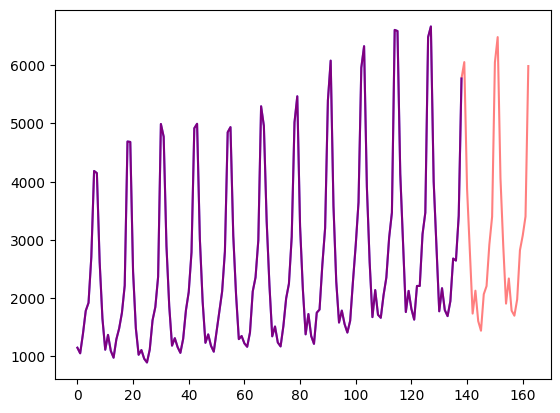
让我们可视化一下:
import matplotlib.pyplot as plt

figure, axes = plt.subplots()
axes.plot(train_example["target"], color="blue")
axes.plot(validation_example["target"], color="red", alpha=0.5)

plt.show()
下面拆分数据:
train_dataset = dataset["train"]
test_dataset = dataset["test"]
将 start 更新为 pd.Period
我们要做的第一件事是根据数据的 freq 值将每个时间序列的 start 特征转换为 pandas 的 Period 索引:
from functools import lru_cache

import pandas as pd
import numpy as np

@lru_cache(10_000)
def convert_to_pandas_period(date, freq):
    return pd.Period(date, freq)

def transform_start_field(batch, freq):
    batch["start"] = [convert_to_pandas_period(date, freq) for date in batch["start"]]
    return batch
这里我们使用 datasets 的 set_transform 来实现:
from functools import partial

train_dataset.set_transform(partial(transform_start_field, freq=freq))
test_dataset.set_transform(partial(transform_start_field, freq=freq))
定义模型
接下来,让我们实例化一个模型。该模型将从头开始训练,因此我们不使用 from_pretrained 方法,而是从 config 中随机初始化模型。
我们为模型指定了几个附加参数:
prediction_length(在我们的例子中是24个月) : 这是 Transformer 的解码器将学习预测的范围;context_length: 如果未指定context_length,模型会将context_length(编码器的输入) 设置为等于prediction_length;- 给定频率的
lags(滞后): 这将决定模型“回头看”的程度,也会作为附加特征。例如对于Daily频率,我们可能会考虑回顾[1, 2, 7, 30, ...],也就是回顾 1、2……天的数据,而对于 Minute数据,我们可能会考虑[1, 30, 60, 60*24, ...]等; - 时间特征的数量: 在我们的例子中设置为
2,因为我们将添加MonthOfYear和Age特征; - 静态类别型特征的数量: 在我们的例子中,这将只是
1,因为我们将添加一个“时间序列 ID”特征; - 基数: 将每个静态类别型特征的值的数量构成一个列表,对于本例来说将是
[366],因为我们有 366 个不同的时间序列; - 嵌入维度: 每个静态类别型特征的嵌入维度,也是构成列表。例如
[3]意味着模型将为每个366时间序列 (区域) 学习大小为3的嵌入向量。
让我们使用 GluonTS 为给定频率 (“每月”) 提供的默认滞后值:
from gluonts.time_feature import get_lags_for_frequency

lags_sequence = get_lags_for_frequency(freq)
print(lags_sequence)

>>> [1, 2, 3, 4, 5, 6, 7, 11, 12, 13, 23, 24, 25, 35, 36, 37]
这意味着我们每个时间步将回顾长达 37 个月的数据,作为附加特征。
我们还检查 GluonTS 为我们提供的默认时间特征:
from gluonts.time_feature import time_features_from_frequency_str

time_features = time_features_from_frequency_str(freq)
print(time_features)

>>> [<function month_of_year at 0x7fa496d0ca70>]
在这种情况下,只有一个特征,即“一年中的月份”。这意味着对于每个时间步长,我们将添加月份作为标量值 (例如,如果时间戳为 "january",则为 1;如果时间戳为 "february",则为 2,等等) 。
我们现在准备好定义模型需要的所有内容了:
from transformers import TimeSeriesTransformerConfig, TimeSeriesTransformerForPrediction

config = TimeSeriesTransformerConfig(
    prediction_length=prediction_length,
    # context length:
    context_length=prediction_length * 2,
    # lags coming from helper given the freq:
    lags_sequence=lags_sequence,
    # we'll add 2 time features ("month of year" and "age", see further):
    num_time_features=len(time_features) + 1,
    # we have a single static categorical feature, namely time series ID:
    num_static_categorical_features=1,
    # it has 366 possible values:
    cardinality=[len(train_dataset)],
    # the model will learn an embedding of size 2 for each of the 366 possible values:
    embedding_dimension=[2],

    # transformer params:
    encoder_layers=4,
    decoder_layers=4,
    d_model=32,
)

model = TimeSeriesTransformerForPrediction(config)
请注意,与 🤗 Transformers 库中的其他模型类似,TimeSeriesTransformerModel 对应于没有任何顶部前置头的编码器-解码器 Transformer,而 TimeSeriesTransformerForPrediction 对应于顶部有一个分布前置头 (distribution head) 的 TimeSeriesTransformerForPrediction。默认情况下,该模型使用 Student-t 分布 (也可以自行配置):
model.config.distribution_output

>>> student_t
这是具体实现层面与用于 NLP 的 Transformers 的一个重要区别,其中头部通常由一个固定的分类分布组成,实现为 nn.Linear 层。
定义转换
接下来,我们定义数据的转换,尤其是需要基于样本数据集或通用数据集来创建其中的时间特征。
同样,我们用到了 GluonTS 库。这里定义了一个 Chain (有点类似于图像训练的 torchvision.transforms.Compose) 。它允许我们将多个转换组合到一个流水线中。
from gluonts.time_feature import (
    time_features_from_frequency_str,
    TimeFeature,
    get_lags_for_frequency,
)
from gluonts.dataset.field_names import FieldName
from gluonts.transform import (
    AddAgeFeature,
    AddObservedValuesIndicator,
    AddTimeFeatures,
    AsNumpyArray,
    Chain,
    ExpectedNumInstanceSampler,
    InstanceSplitter,
    RemoveFields,
    SelectFields,
    SetField,
    TestSplitSampler,
    Transformation,
    ValidationSplitSampler,
    VstackFeatures,
    RenameFields,
)
下面的转换代码带有注释供大家查看具体的操作步骤。从全局来说,我们将迭代数据集的各个时间序列并添加、删除某些字段或特征:
from transformers import PretrainedConfig

def create_transformation(freq: str, config: PretrainedConfig) -> Transformation:
    remove_field_names = []
    if config.num_static_real_features == 0:
        remove_field_names.append(FieldName.FEAT_STATIC_REAL)
    if config.num_dynamic_real_features == 0:
        remove_field_names.append(FieldName.FEAT_DYNAMIC_REAL)
    if config.num_static_categorical_features == 0:
        remove_field_names.append(FieldName.FEAT_STATIC_CAT)

    # a bit like torchvision.transforms.Compose
    return Chain(
        # step 1: remove static/dynamic fields if not specified
        [RemoveFields(field_names=remove_field_names)]
        # step 2: convert the data to NumPy (potentially not needed)
        + (
            [
                AsNumpyArray(
                    field=FieldName.FEAT_STATIC_CAT,
                    expected_ndim=1,
                    dtype=int,
                )
            ]
            if config.num_static_categorical_features > 0
            else []
        )
        + (
            [
                AsNumpyArray(
                    field=FieldName.FEAT_STATIC_REAL,
                    expected_ndim=1,
                )
            ]
            if config.num_static_real_features > 0
            else []
        )
        + [
            AsNumpyArray(
                field=FieldName.TARGET,
                # we expect an extra dim for the multivariate case:
                expected_ndim=1 if config.input_size == 1 else 2,
            ),
            # step 3: handle the NaN's by filling in the target with zero
            # and return the mask (which is in the observed values)
            # true for observed values, false for nan's
            # the decoder uses this mask (no loss is incurred for unobserved values)
            # see loss_weights inside the xxxForPrediction model
            AddObservedValuesIndicator(
                target_field=FieldName.TARGET,
                output_field=FieldName.OBSERVED_VALUES,
            ),
            # step 4: add temporal features based on freq of the dataset
            # month of year in the case when freq="M"
            # these serve as positional encodings
            AddTimeFeatures(
                start_field=FieldName.START,
                target_field=FieldName.TARGET,
                output_field=FieldName.FEAT_TIME,
                time_features=time_features_from_frequency_str(freq),
                pred_length=config.prediction_length,
            ),
            # step 5: add another temporal feature (just a single number)
            # tells the model where in its life the value of the time series is,
            # sort of a running counter
            AddAgeFeature(
                target_field=FieldName.TARGET,
                output_field=FieldName.FEAT_AGE,
                pred_length=config.prediction_length,
                log_scale=True,
            ),
            # step 6: vertically stack all the temporal features into the key FEAT_TIME
            VstackFeatures(
                output_field=FieldName.FEAT_TIME,
                input_fields=[FieldName.FEAT_TIME, FieldName.FEAT_AGE]
                + (
                    [FieldName.FEAT_DYNAMIC_REAL]
                    if config.num_dynamic_real_features > 0
                    else []
                ),
            ),
            # step 7: rename to match HuggingFace names
            RenameFields(
                mapping={
                    FieldName.FEAT_STATIC_CAT: "static_categorical_features",
                    FieldName.FEAT_STATIC_REAL: "static_real_features",
                    FieldName.FEAT_TIME: "time_features",
                    FieldName.TARGET: "values",
                    FieldName.OBSERVED_VALUES: "observed_mask",
                }
            ),
        ]
    )
定义 InstanceSplitter
对于训练、验证、测试步骤,接下来我们创建一个 InstanceSplitter,用于从数据集中对窗口进行采样 (因为由于时间和内存限制,我们无法将整个历史值传递给 Transformer)。
实例拆分器从数据中随机采样大小为 context_length 和后续大小为 prediction_length 的窗口,并将 past_ 或 future_ 键附加到各个窗口的任何临时键。这确保了 values 被拆分为 past_values 和后续的 future_values 键,它们将分别用作编码器和解码器的输入。同样我们还需要修改 time_series_fields 参数中的所有键:
from gluonts.transform.sampler import InstanceSampler
from typing import Optional

def create_instance_splitter(
    config: PretrainedConfig,
    mode: str,
    train_sampler: Optional[InstanceSampler] = None,
    validation_sampler: Optional[InstanceSampler] = None,
) -> Transformation:
    assert mode in ["train", "validation", "test"]

    instance_sampler = {
        "train": train_sampler
        or ExpectedNumInstanceSampler(
            num_instances=1.0, min_future=config.prediction_length
        ),
        "validation": validation_sampler
        or ValidationSplitSampler(min_future=config.prediction_length),
        "test": TestSplitSampler(),
    }[mode]

    return InstanceSplitter(
        target_field="values",
        is_pad_field=FieldName.IS_PAD,
        start_field=FieldName.START,
        forecast_start_field=FieldName.FORECAST_START,
        instance_sampler=instance_sampler,
        past_length=config.context_length + max(config.lags_sequence),
        future_length=config.prediction_length,
        time_series_fields=["time_features", "observed_mask"],
    )
创建 PyTorch 数据加载器
有了数据,下一步需要创建 PyTorch DataLoaders。它允许我们批量处理成对的 (输入, 输出) 数据,即 (past_values, future_values)。
from typing import Iterable

import torch
from gluonts.itertools import Cached, Cyclic
from gluonts.dataset.loader import as_stacked_batches


def create_train_dataloader(
    config: PretrainedConfig,
    freq,
    data,
    batch_size: int,
    num_batches_per_epoch: int,
    shuffle_buffer_length: Optional[int] = None,
    cache_data: bool = True,
    **kwargs,
) -> Iterable:
    PREDICTION_INPUT_NAMES = [
        "past_time_features",
        "past_values",
        "past_observed_mask",
        "future_time_features",
    ]
    if config.num_static_categorical_features > 0:
        PREDICTION_INPUT_NAMES.append("static_categorical_features")

    if config.num_static_real_features > 0:
        PREDICTION_INPUT_NAMES.append("static_real_features")

    TRAINING_INPUT_NAMES = PREDICTION_INPUT_NAMES + [
        "future_values",
        "future_observed_mask",
    ]

    transformation = create_transformation(freq, config)
    transformed_data = transformation.apply(data, is_train=True)
    if cache_data:
        transformed_data = Cached(transformed_data)

    # we initialize a Training instance
    instance_splitter = create_instance_splitter(config, "train")

    # the instance splitter will sample a window of
    # context length + lags + prediction length (from the 366 possible transformed time series)
    # randomly from within the target time series and return an iterator.
    stream = Cyclic(transformed_data).stream()
    training_instances = instance_splitter.apply(
        stream, is_train=True
    )

    return as_stacked_batches(
        training_instances,
        batch_size=batch_size,
        shuffle_buffer_length=shuffle_buffer_length,
        field_names=TRAINING_INPUT_NAMES,
        output_type=torch.tensor,
        num_batches_per_epoch=num_batches_per_epoch,
    )
def create_test_dataloader(
    config: PretrainedConfig,
    freq,
    data,
    batch_size: int,
    **kwargs,
):
    PREDICTION_INPUT_NAMES = [
        "past_time_features",
        "past_values",
        "past_observed_mask",
        "future_time_features",
    ]
    if config.num_static_categorical_features > 0:
        PREDICTION_INPUT_NAMES.append("static_categorical_features")

    if config.num_static_real_features > 0:
        PREDICTION_INPUT_NAMES.append("static_real_features")

    transformation = create_transformation(freq, config)
    transformed_data = transformation.apply(data, is_train=False)

    # we create a Test Instance splitter which will sample the very last
    # context window seen during training only for the encoder.
    instance_sampler = create_instance_splitter(config, "test")

    # we apply the transformations in test mode
    testing_instances = instance_sampler.apply(transformed_data, is_train=False)

    return as_stacked_batches(
        testing_instances,
        batch_size=batch_size,
        output_type=torch.tensor,
        field_names=PREDICTION_INPUT_NAMES,
    )
train_dataloader = create_train_dataloader(
    config=config,
    freq=freq,
    data=train_dataset,
    batch_size=256,
    num_batches_per_epoch=100,
)

test_dataloader = create_test_dataloader(
    config=config,
    freq=freq,
    data=test_dataset,
    batch_size=64,
)
让我们检查第一批:
batch = next(iter(train_dataloader))
for k, v in batch.items():
    print(k, v.shape, v.type())

>>> past_time_features torch.Size([256, 85, 2]) torch.FloatTensor
    past_values torch.Size([256, 85]) torch.FloatTensor
    past_observed_mask torch.Size([256, 85]) torch.FloatTensor
    future_time_features torch.Size([256, 24, 2]) torch.FloatTensor
    static_categorical_features torch.Size([256, 1]) torch.LongTensor
    future_values torch.Size([256, 24]) torch.FloatTensor
    future_observed_mask torch.Size([256, 24]) torch.FloatTensor
可以看出,我们没有将 input_ids 和 attention_mask 提供给编码器 (训练 NLP 模型时也是这种情况),而是提供 past_values,以及 past_observed_mask、past_time_features、static_categorical_features 和 static_real_features 几项数据。
解码器的输入包括 future_values、future_observed_mask 和 future_time_features。future_values 可以看作等同于 NLP 训练中的 decoder_input_ids。
我们可以参考 Time Series Transformer 文档 以获得对它们中每一个的详细解释。
前向传播
让我们对刚刚创建的批次执行一次前向传播:
# perform forward pass
outputs = model(
    past_values=batch["past_values"],
    past_time_features=batch["past_time_features"],
    past_observed_mask=batch["past_observed_mask"],
    static_categorical_features=batch["static_categorical_features"]
    if config.num_static_categorical_features > 0
    else None,
    static_real_features=batch["static_real_features"]
    if config.num_static_real_features > 0
    else None,
    future_values=batch["future_values"],
    future_time_features=batch["future_time_features"],
    future_observed_mask=batch["future_observed_mask"],
    output_hidden_states=True,
)
print("Loss:", outputs.loss.item())

>>> Loss: 9.069628715515137
目前,该模型返回了损失值。这是由于解码器会自动将 future_values 向右移动一个位置以获得标签。这允许计算预测结果和标签值之间的误差。
另请注意,解码器使用 Causal Mask 来避免预测未来,因为它需要预测的值在 future_values 张量中。
训练模型
是时候训练模型了!我们将使用标准的 PyTorch 训练循环。
这里我们用到了 🤗 Accelerate 库,它会自动将模型、优化器和数据加载器放置在适当的 device 上。
from accelerate import Accelerator
from torch.optim import AdamW

accelerator = Accelerator()
device = accelerator.device

model.to(device)
optimizer = AdamW(model.parameters(), lr=6e-4, betas=(0.9, 0.95), weight_decay=1e-1)

model, optimizer, train_dataloader = accelerator.prepare(
    model,
    optimizer,
    train_dataloader,
)

model.train()
for epoch in range(40):
    for idx, batch in enumerate(train_dataloader):
        optimizer.zero_grad()
        outputs = model(
            static_categorical_features=batch["static_categorical_features"].to(device)
            if config.num_static_categorical_features > 0
            else None,
            static_real_features=batch["static_real_features"].to(device)
            if config.num_static_real_features > 0
            else None,
            past_time_features=batch["past_time_features"].to(device),
            past_values=batch["past_values"].to(device),
            future_time_features=batch["future_time_features"].to(device),
            future_values=batch["future_values"].to(device),
            past_observed_mask=batch["past_observed_mask"].to(device),
            future_observed_mask=batch["future_observed_mask"].to(device),
        )
        loss = outputs.loss

        # Backpropagation
        accelerator.backward(loss)
        optimizer.step()

        if idx % 100 == 0:
            print(loss.item())
推理
在推理时,建议使用 generate() 方法进行自回归生成,类似于 NLP 模型。
预测的过程会从测试实例采样器中获得数据。采样器会将数据集的每个时间序列的最后 context_length 那么长时间的数据采样出来,然后输入模型。请注意,这里需要把提前已知的 future_time_features 传递给解码器。
该模型将从预测分布中自回归采样一定数量的值,并将它们传回解码器最终得到预测输出:
model.eval()

forecasts = []

for batch in test_dataloader:
    outputs = model.generate(
        static_categorical_features=batch["static_categorical_features"].to(device)
        if config.num_static_categorical_features > 0
        else None,
        static_real_features=batch["static_real_features"].to(device)
        if config.num_static_real_features > 0
        else None,
        past_time_features=batch["past_time_features"].to(device),
        past_values=batch["past_values"].to(device),
        future_time_features=batch["future_time_features"].to(device),
        past_observed_mask=batch["past_observed_mask"].to(device),
    )
    forecasts.append(outputs.sequences.cpu().numpy())
该模型输出一个表示结构的张量 (batch_size, number of samples, prediction length)。
下面的输出说明: 对于大小为 64 的批次中的每个示例,我们将获得接下来 24 个月内的 100 个可能的值:
forecasts[0].shape

>>> (64, 100, 24)
我们将垂直堆叠它们,以获得测试数据集中所有时间序列的预测:
forecasts = np.vstack(forecasts)
print(forecasts.shape)

>>> (366, 100, 24)
我们可以根据测试集中存在的样本值,根据真实情况评估生成的预测。这里我们使用数据集中的每个时间序列的 MASE 和 sMAPE 指标 (metrics) 来评估:
from evaluate import load
from gluonts.time_feature import get_seasonality

mase_metric = load("evaluate-metric/mase")
smape_metric = load("evaluate-metric/smape")

forecast_median = np.median(forecasts, 1)

mase_metrics = []
smape_metrics = []
for item_id, ts in enumerate(test_dataset):
    training_data = ts["target"][:-prediction_length]
    ground_truth = ts["target"][-prediction_length:]
    mase = mase_metric.compute(
        predictions=forecast_median[item_id],
        references=np.array(ground_truth),
        training=np.array(training_data),
        periodicity=get_seasonality(freq))
    mase_metrics.append(mase["mase"])

    smape = smape_metric.compute(
        predictions=forecast_median[item_id],
        references=np.array(ground_truth),
    )
    smape_metrics.append(smape["smape"])
print(f"MASE: {np.mean(mase_metrics)}")

>>> MASE: 1.2564196892177717

print(f"sMAPE: {np.mean(smape_metrics)}")

>>> sMAPE: 0.1609541520852549
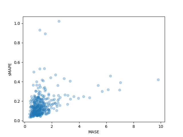
我们还可以单独绘制数据集中每个时间序列的结果指标,并观察到其中少数时间序列对最终测试指标的影响很大:
plt.scatter(mase_metrics, smape_metrics, alpha=0.3)
plt.xlabel("MASE")
plt.ylabel("sMAPE")
plt.show()
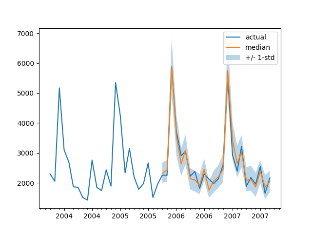
为了根据基本事实测试数据绘制任何时间序列的预测,我们定义了以下辅助绘图函数:
import matplotlib.dates as mdates

def plot(ts_index):
    fig, ax = plt.subplots()

    index = pd.period_range(
        start=test_dataset[ts_index][FieldName.START],
        periods=len(test_dataset[ts_index][FieldName.TARGET]),
        freq=freq,
    ).to_timestamp()

    # Major ticks every half year, minor ticks every month,
    ax.xaxis.set_major_locator(mdates.MonthLocator(bymonth=(1, 7)))
    ax.xaxis.set_minor_locator(mdates.MonthLocator())

    ax.plot(
        index[-2*prediction_length:],
        test_dataset[ts_index]["target"][-2*prediction_length:],
        label="actual",
    )

    plt.plot(
        index[-prediction_length:],
        np.median(forecasts[ts_index], axis=0),
        label="median",
    )

    plt.fill_between(
        index[-prediction_length:],
        forecasts[ts_index].mean(0) - forecasts[ts_index].std(axis=0),
        forecasts[ts_index].mean(0) + forecasts[ts_index].std(axis=0),
        alpha=0.3,
        interpolate=True,
        label="+/- 1-std",
    )
    plt.legend()
    plt.show()
例如:
plot(334)
我们如何与其他模型进行比较?Monash Time Series Repository 有一个测试集 MASE 指标的比较表。我们可以将自己的结果添加到其中作比较:
| Dataset | SES | Theta | TBATS | ETS | (DHR-)ARIMA | PR | CatBoost | FFNN | DeepAR | N-BEATS | WaveNet | Transformer (Our) |
|---|---|---|---|---|---|---|---|---|---|---|---|---|
| Tourism Monthly | 3.306 | 1.649 | 1.751 | 1.526 | 1.589 | 1.678 | 1.699 | 1.582 | 1.409 | 1.574 | 1.482 | 1.256 |
请注意,我们的模型击败了所有已知的其他模型 (另请参见相应 论文 中的表 2) ,并且我们没有做任何超参数优化。我们仅仅花了 40 个完整训练调参周期来训练 Transformer。
当然,我们应该谦虚。从历史发展的角度来看,现在认为神经网络解决时间序列预测问题是正途,就好比当年的论文得出了 “你需要的就是 XGBoost” 的结论。我们只是很好奇,想看看神经网络能带我们走多远,以及 Transformer 是否会在这个领域发挥作用。这个特定的数据集似乎表明它绝对值得探索。
下一步
我们鼓励读者尝试我们的 Jupyter Notebook 和来自 Hugging Face Hub 的其他时间序列数据集,并替换适当的频率和预测长度参数。对于您的数据集,需要将它们转换为 GluonTS 的惯用格式,在他们的 文档 里有非常清晰的说明。我们还准备了一个示例 Notebook,向您展示如何将数据集转换为 🤗 Hugging Face 数据集格式。
正如时间序列研究人员所知,人们对“将基于 Transformer 的模型应用于时间序列”问题很感兴趣。传统 vanilla Transformer 只是众多基于注意力 (Attention) 的模型之一,因此需要向库中补充更多模型。
目前没有什么能妨碍我们继续探索对多变量时间序列 (multivariate time series) 进行建模,但是为此需要使用多变量分布头 (multivariate distribution head) 来实例化模型。目前已经支持了对角独立分布 (diagonal independent distributions),后续会增加其他多元分布支持。请继续关注未来的博客文章以及其中的教程。
路线图上的另一件事是时间序列分类。这需要将带有分类头的时间序列模型添加到库中,例如用于异常检测这类任务。
当前的模型会假设日期时间和时间序列值都存在,但在现实中这可能不能完全满足。例如 WOODS 给出的神经科学数据集。因此,我们还需要对当前模型进行泛化,使某些输入在整个流水线中可选。
最后,NLP/CV 领域从 大型预训练模型 中获益匪浅,但据我们所知,时间序列领域并非如此。基于 Transformer 的模型似乎是这一研究方向的必然之选,我们迫不及待地想看看研究人员和从业者会发现哪些突破!