What's Automatic Differentiation?

Clarification

---

Before we begin, this blog is technically and mathematically involved—covering topics related to Calculus, Linear Algebra, and machine learning (ML). For example, we discuss partial derivatives, gradients, multivariate functions, and loss functions. To save on time, I assume you have some basic knowledge or familiarity with these subjects.

TL;DR

---

The main premise behind this blog is to highlight automatic differentiation (AD) and how it can be utilized for gradient-based optimization seen in training neural networks. I cover:

• Numeric Differentiation as a process approximating the derivative of a function that's avoided for neural network optimization because of issues like truncation and round-off error.

• Symbolic Differentiation being a systematic way to derive the derivative of an expression through transformations. It's avoided for gradient-based optimization because of code constraints, expression swell, and repeated computations.

• Automatic Differentiation (AD) as a method augmenting arithmetic computation by interleaving derivatives with the elementary operations of functions. I also describe the evaluation trace and computational graph—useful in forward and reverse mode AD.

• Forward Mode AD being one way to apply automatic differentiation by computing the partial derivatives of variables during the forward pass of functions. It's observed to be useful, but not optimal for gradient-based optimization since it's slow under certain conditions.

• Reverse Mode AD as the alternative mode that computes the partial derivatives of variables during the reverse pass, after function evaluation. This mode is faster than forward mode under the context of optimizing neural networks due to features like the reverse pass and vector-Jacobian product.

Wrapping up the blog, I implement forward and reverse mode AD in python using operator overloading. Gaining insight on how AD is built in code, I contrast the implementation with that of a familiar ML framework.

Introduction

---

In ML, neural networks implement a breadth of mathematical, and even scientific techniques, to make the AI tools we have today (e.g. LLMs) possible. The field has evolved from using simple neural networks to classify handwritten digits, to transformer architectures that are sometimes considered "sentient". What remains at its core is solving the problem of optimization—that is, how can we teach these models to learn?

There's likely better ways to solve this problem that some genius will one day discover, but the consensus today is through gradient descent. Gradient descent is an optimization algorithm that aims to improve a model's performance through iterative incremental steps. Here's a breakdown:

Gradient Descent

1. Using an objective [loss] function, compute the loss (error) between a model's predictions over a set of inputs and the ground truth of those inputs.

2. Find the model's influence on the loss by computing the partial derivatives of the loss w.r.t. every parameter of the model (the gradients).

3. Move the model's parameters in the direction that minimizes the loss by subtracting each parameter with its respective gradient scaled by a hyperparameter called the learning rate.

4. Clear all the gradients, and repeat the process until the model converges; in better words, until the model no longer improves and achieves optimal performance.

This process has evidently built robust deep neural networks, however, it requires a difficult procedure, and that's finding the gradients to update the model's parameters. In a mathematical sense, how can we differentiate the loss w.r.t. the model's parameters? To that, I welcome automatic differentiation.

In this blog, I'll provide an explanation as to what automatic differentiation is, and we'll also take a dive into its implementation. But before we progress further, we need to understand two alternative approaches and why they fail to meet the demands of gradient-based optimization for neural networks, numeric and symbolic differentiation.

Numeric Differentiation

---

Numeric differentiation is one approach we can utilize to help us compute gradients to optimize neural networks by using the limit definition of a derivative.

$$\begin{array}{cccc}& \frac{df}{dx}=\underset{h\to 0}{\lim }\frac{f(x+h)-f(x)}{h}& & \text{(1)}\end{array}\backslash tag\{1\}\backslash frac\{df\}\{dx\}\; =\; \backslash lim\_\{\; h\backslash to\; 0\}\backslash frac\{f(x\; +\; h)\; -\; f(x)\}\{h\}$$

To evaluate the derivative of a function $f:\mathbb{R}\to \mathbb{R}f:\; \backslash R\; \backslash to\; \backslash R$ for an input $xx$, we find the slope of the tangent line at $xx$. The tangent line can be broken down into the quotient of the rise and run of the function at $xx$. To compute the rise, we evaluate the function at two inputs, one with the original input and the other with the input nudged by a small constant $hh$; this is observed in the numerator of eq. 1. Next, we divide by the run; since we pushed the input by $hh$, the run is $hh$. As $hh$ approaches zero, by taking the limit, the approximation for the derivative of $f(x)f(x)$ at $xx$ becomes more accurate.

In practice, neural networks apply arithmetic operations to multi-dimensional arrays—tensors as they're often called—and it wouldn't make sense to programmatically take the limit, so we discard the limit and rewrite the expression to operate on a network's parameters.

$$\begin{array}{cccc}& \frac{\mathrm{\partial }f}{\mathrm{\partial }{\mathbf{\theta }}_i}\approx \frac{f(\mathbf{\theta }+h\cdot {\mathbf{e}}_i)-f(\mathbf{\theta })}{h}+O(h)& & \text{(2)}\end{array}\backslash tag\{2\}\backslash frac\{\backslash partial\; f\}\{\backslash partial\; \backslash bold\{\backslash theta\}\_i\}\; \backslash approx\; \backslash frac\{f(\backslash bold\{\backslash theta\}\; +\; h\; \backslash cdot\; \backslash bold\{e\}\_i)\; -\; f(\backslash bold\{\backslash theta\})\}\{h\}\; +\; O(h)$$

Above is the forward difference method to compute the partial derivative of a multivariate function
$f:{\mathbb{R}}^n\to \mathbb{R}f:\; \backslash R^\{n\}\; \backslash to\; \backslash R$ w.r.t. a single parameter $\theta {}_i\backslash theta\{\_i\}$, from a vector of parameters $\mathbf{\theta }\backslash bold\{\backslash theta\}$. The symbol ${\mathbf{e}}_i\backslash bold\{e\}\_i$ represents a unit vector, where the $i\text{-th}i\; \backslash text\{-th\}$ element is one while all other elements are zero. Computing the partial derivative for the $i\text{-th}i\; \backslash text\{-\{th\}\}$ parameter in $\mathbf{\theta }\backslash bold\{\backslash theta\}$ is now as easy as evaluating eq. 2 with $h\approx 0h\; \backslash approx\; 0$. In the realms of neural networks, $ff$ is a representation of the objective loss function, while $\mathbf{\theta }\backslash bold\{\backslash theta\}$ is the parameterization of the model. By evaluating eq. 2 on all the model's parameters, we'd obtain the gradients required for one step of gradient descent.

What I have yet to mention is the big-O term added to the end of eq. 2. This symbol—outside the domain of time and space complexity for algorithms—is a function on $hh$ that expresses the truncation error. Truncation error is defined as the error caused by cutting off some values from the Taylor series of $\frac{\mathrm{\partial }f}{\mathrm{\partial }{\mathbf{\theta }}_i}\backslash frac\{\backslash partial\; f\}\{\backslash partial\; \backslash bold\{\backslash theta\}\_i\}$. More concretely, because we're taking an approximation for the partial derivative for $\theta {}_i\backslash theta\{\_i\}$ using $hh$, we're mis-approximating it with some error dependent on $hh$. Additionally, the truncation error is directly proportional to $hh$, meaning whatever factor $hh$ is scaled by, the truncation error will be scaled by the same factor.

Now, there's ways to minimize this error. For starters, we can change our approximation to the central difference method seen below.

$$\begin{array}{cccc}& \frac{\mathrm{\partial }f}{\mathrm{\partial }{\mathbf{\theta }}_i}\approx \frac{f(\mathbf{\theta }+h\cdot {\mathbf{e}}_i)-f(\mathbf{\theta }-h\cdot {\mathbf{e}}_i)}{2h}+O(h^2)& & \text{(3)}\end{array}\backslash tag\{3\}\backslash frac\{\backslash partial\; f\}\{\backslash partial\; \backslash bold\{\backslash theta\}\_i\}\; \backslash approx\; \backslash frac\{f(\backslash bold\{\backslash theta\}\; +\; h\; \backslash cdot\; \backslash bold\{e\}\_i)\; -\; f(\backslash bold\{\backslash theta\}\; -\; h\; \backslash cdot\; \backslash bold\{e\}\_i)\}\{2h\}\; +\; O(h^2)$$

The central difference is the combination of the forward difference from eq 2. and the backward difference. By subtracting the backward difference from the forward difference and simplifying, the first order error terms in $O(h)O(h)$ will cancel out, leaving the second order error term as dominant. The error is now proportional to the square of $hh$, meaning if $hh$ decreases by an order of magnitude, the error will decrease by two orders of magnitude.

Derivative Approximations

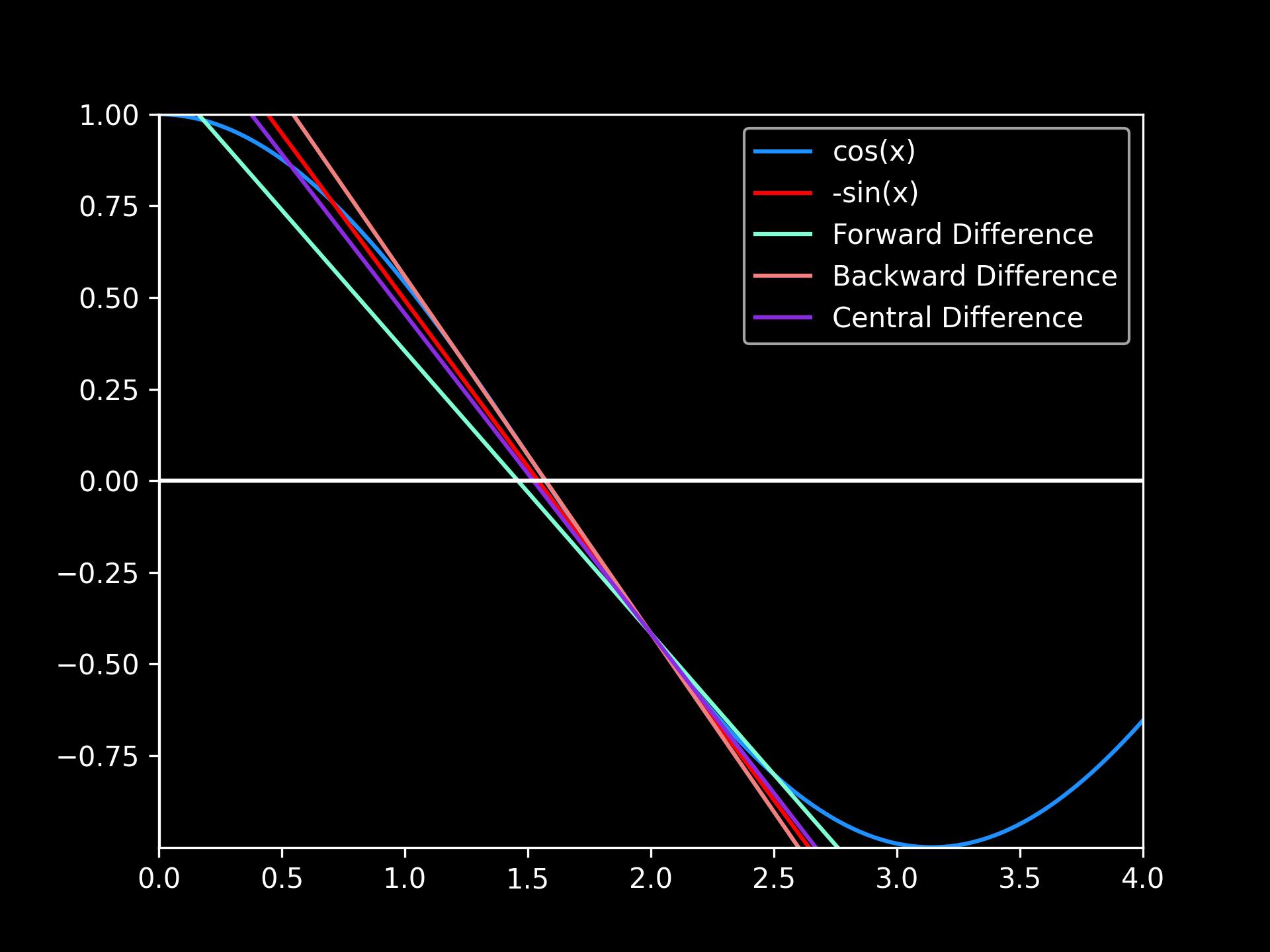
Derivative Approximations: pictured are the derivatives for $cos(x)cos(x)$ at $x=2x\; =\; 2$, using $h=0.5h\; =\; 0.5$ for the numeric differentiation methods (all computations used 32-bit floats). The graph highlights a better approximation in taking the central difference over the forward and backward difference. In addition, the discrepancies between the actual derivative $-\sin (2)-\; \backslash sin(2)$ and the approximated derivatives caused by truncation error can be viewed.

As another way to stabilize this approach, we could just reduce $hh$ since the truncation error becomes nonexistent as $h\approx 0h\; \backslash approx\; 0$. In theory, this should eliminate the error we're facing with numeric differentiation. However, doing such has side-effects leading us into the next section.

Issues with Numeric Differentiation

---

With an understanding of numeric differentiation, we can explore why it's avoided in the implementation of neural network optimization. In reference to decreasing $hh$ as a solution to mitigate truncation error, we also introduce another error known as round-off error.

Round-off error is the error induced due to the inaccuracies of how numbers can be represented within computers. Standards such as the IEEE 754 have popularized the use of single precision floats (float32) to represent real numbers in programs. Neural networks depend on these representations, however, they're limited. Floats are allocated a fixed amount of space (32 bits in most cases), preventing certain levels of precision for arbitrarily large or small values. Tying this into numerical differentiation, if numbers get too small they'll underflow into zero and lose numerical information in the process.

This is significant because as we try to decrease $hh$ to alleviate the truncation error, we increase our round-off error. In fact, the round-off error is inversely proportional to the scale of $hh$. For example, if we halve $hh$, we double the round-off error. This balance between truncation and round-off error introduces a trade-off to consider when choosing a viable $hh$ to compute accurate gradients.

Truncation vs. Round-off Error

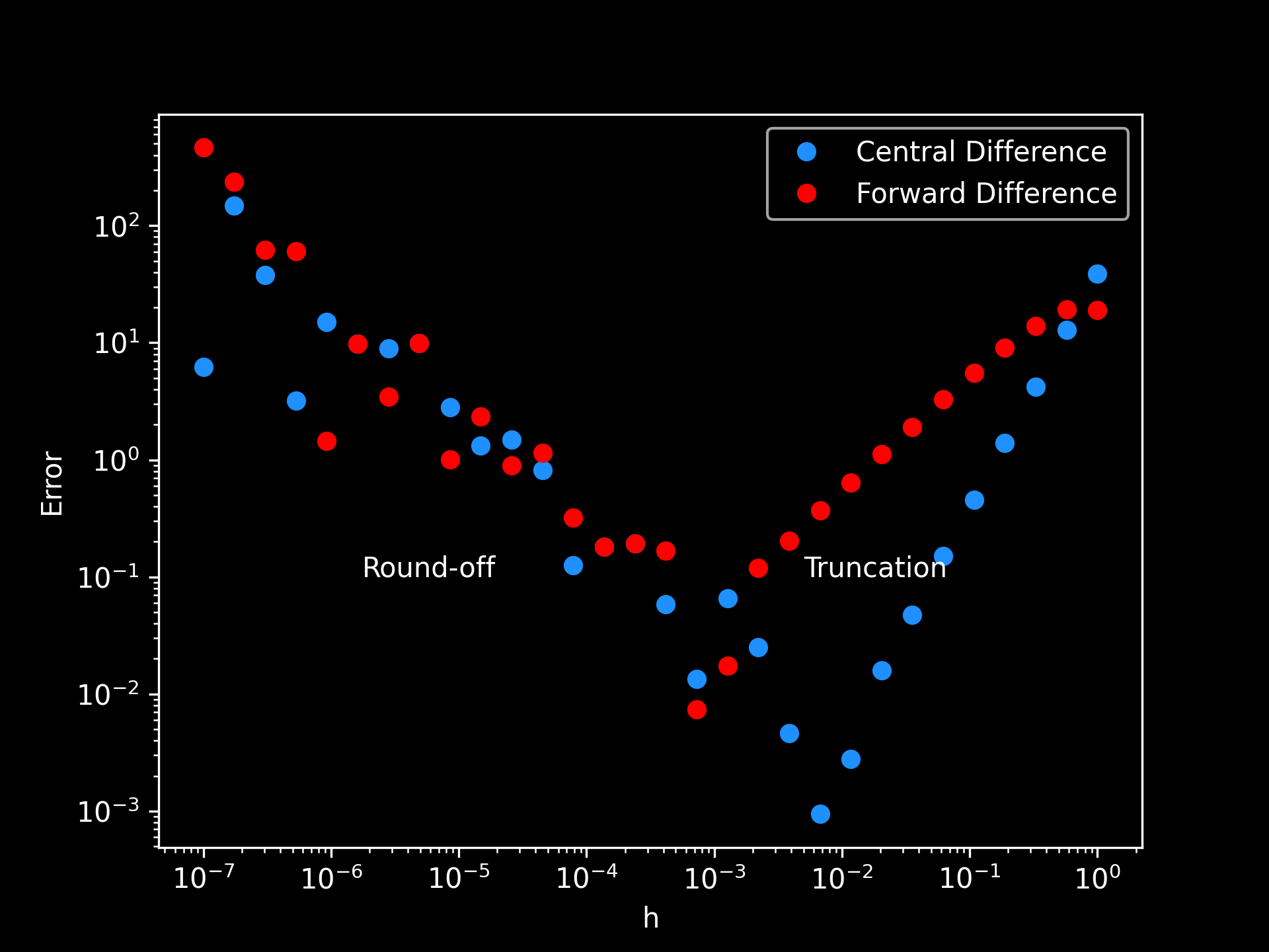
Truncation vs. Round-off Error: above are sampled errors present in the computation of the forward difference method (eq. 2) and the central difference method (eq. 3) for the function $f(x)=(x-10{)}^2(3x^2-3x+1)f(x)\; =\; (x\; -\; 10)^2(3x^2\; -3x\; +\; 1)$. Single precision floating-point values in the range $[10^{-7},1][10^\{-7\},\; 1]$ were used for $hh$. It's seen as $hh$ decreases, the truncation error decreases with the introduction of round-off error and vice-versa when $hh$ grows.

One could make the suggestion of using a higher precision data type (e.g. float64), but this increases hardware constraints due to more memory requirements and additional computations—another tradeoff that's completely unnecessary. Pivoting, another issue arises from the runtime complexity of numerical differentiation.

To actually compute the gradients, we have to evaluate the function of interest. In the case of finding the gradients for a function with $nn$ inputs and a scalar output, we'd require $O(n)O(n)$ operations. This doesn't even consider vector-valued functions seen in neural networks. For example, if we have the function $f:{\mathbb{R}}^n\to {\mathbb{R}}^{m}f:\; \backslash R^\{n\}\; \backslash to\; \backslash R^\{m\}$, we'd require roughly $O(mn)O(mn)$ operations to compute the gradients, making the total computation inefficient for large values of $mm$ and $nn$.

With the context that gradient descent is an iterative process applied to millions or even billions of parameters, we can see that numeric differentiation doesn't scale well enough for neural network optimization. Knowing where it comes short, we can shift towards an alternate approach in symbolic differentiation.

Symbolic Differentiation

---

Symbolic differentiation is the next approach we'll unpack for gradient computation. It's a systematic process that transforms an expression composed of arithmetic operations and symbols, into an expression representing its derivative. This is achieved by applying the derivative rules of Calculus (e.g. sum rule) to closed-form expressions.

In reality, symbolic differentiation is a computer's way of how we hand derive the derivative of an expression. For example with the two functions $ff$ and $gg$ below, we can use Calculus to derive an expression for its derivative.

$$g(x)=cos(x)+2x-e^{x}g(x)=cos(x)+\; 2x\; -\; e^x$$

$$f(g)=4g^{2}f(g)=4g^2$$

$$\begin{array}{cccc}& f(g(x))=4(cos(x)+2x-e^x{)}^2& & \text{(4)}\end{array}\backslash tag\{4\}f(g(x))\; =\; 4(cos(x)+\; 2x\; -\; e^x)^2$$

$$\begin{array}{cccc}& \frac{df}{dx}=\frac{df}{dg}\cdot \frac{dg}{dx}=8(cos(x)+2x-e^x)\cdot (-sin(x)+2-e^x)& & \text{(5)}\end{array}\backslash tag\{5\}\; \backslash frac\{df\}\{dx\}\; =\; \backslash frac\{df\}\{dg\}\; \backslash cdot\; \backslash frac\{dg\}\{dx\}\; =\; 8(cos(x)+2x\; -\; e^x)\; \backslash cdot\; (-sin(x)\; +\; 2-e^x)$$

To find the derivative for an input of $f(g(x))f(g(x))$, we'd just plug it into the transformed expression above and evaluate it. In practice, we'd programmatically implement this process, and the variables represented would be more than just scalars (e.g. vectors, matrices, or tensors). Below is an example of how we'd symbolically differentiate eq. 4 to get eq. 5 using sympy in python*.

from sympy import symbols, cos, exp, diff

x = symbols("x")
fog = 4 * (cos(x) + 2 * x - exp(x)) ** 2
dfdx = diff(fog, x)
print(dfdx)

4*(2*x - exp(x) + cos(x))*(-2*exp(x) - 2*sin(x) + 4)

* The derivative expression might appear different than eq. 5, but they're actually the same. The terms are slightly reordered and the $22$ from $\frac{df}{dg}\backslash frac\{df\}\{dg\}$ gets distributed to $\frac{dg}{dx}\backslash frac\{dg\}\{dx\}$.

This solves the issue of numerical inaccuracies and instabilities seen in numerical differentiation (view Derivative Approximations and Truncation vs. Round-off Error depictions) because we have an expression that can directly compute the gradients of a function. Still, we face issues limiting its viability for optimizing neural networks that we will dissolve in the next section.

Issues with Symbolic Differentiation

---

The leading issue we can see with symbolic differentiation is expression swell. Expression swell causes the derivative expression, through transformations, to exponentially grow as a penalty of systematically applying the derivative rules to the original expression. Take for example the product rule below.

$$\frac{d}{dx}f(x)g(x)=f^{\mathrm{\prime }}(x)g(x)+g^{\mathrm{\prime }}(x)f(x)\backslash frac\{d\}\{dx\}f(x)g(x)=f\text{'}(x)g(x)\; +\; g\text{'}(x)f(x)$$

The derivative expression has grown not only in terms, but in computation. This doesn't even consider that either $ff$ or $gg$ can be complex functions themselves—potentially adding more expression swell.

We saw a bit of expression swell when we derived $\frac{df}{dx}\backslash frac\{df\}\{dx\}$, and this was a relatively simple function. Now imagine trying to do the same for many composite functions that may apply the derivative rules over and over again. Doing this, knowing neural networks represent many complex composite functions, is extremely impractical.

Expression Swell

$$f(x)=\frac{e^{wx+b}+e^{-(wx+b)}}{e^{wx+b}-e^{-(wx+b)}}f(x)\; =\; \backslash frac\{e^\{wx+b\}\; +\; e^\{-(wx+b)\}\}\{e^\{wx+b\}\; -\; e^\{-(wx+b)\}\}$$

$$\frac{\mathrm{\partial }f}{\mathrm{\partial }w}=\frac{(-x{e}^{-b-wx}-x{e}^{b+wx})(e^{-b-wx}+e^{b+wx})}{(-e^{-b-wx}+e^{b+wx}{)}^2}+\frac{-x{e}^{-b-wx}+x{e}^{b+wx}}{-e^{-b-wx}+e^{b+wx}}\backslash frac\{\backslash partial\; f\}\{\backslash partial\; w\}\; =\; \backslash frac\{(-\; x\; e^\{-\; b\; -\; w\; x\}\; -\; x\; e^\{b\; +\; w\; x\})\; (e^\{-\; b\; -\; w\; x\}\; +\; e^\{b\; +\; w\; x\})\}\{(-\; e^\{-\; b\; -\; w\; x\}\; +\; e^\{b\; +\; w\; x\})^\{2\}\}\; +\; \backslash frac\{-\; x\; e^\{-\; b\; -\; w\; x\}\; +\; x\; e^\{b\; +\; w\; x\}\}\{-\; e^\{-\; b\; -\; w\; x\}\; +\; e^\{b\; +\; w\; x\}\}$$

Expression Swell: shown is a linear projection seen in neural networks, followed by the nonlinear activation function $\text{tanh}\backslash text\{tanh\}$. It's shown, without simplification and optimizations, that finding the gradients to update the weights $ww$ can lead to an egregious amount of expression swell and duplicate computations.

Another drawback faced is the fact that symbolic differentiation is confined to closed-form expressions. What makes programming useful is the ability to use control flow to change how a program behaves depending on its state, and the same principle is often applied to neural networks. What if we wanted to change how an operation is applied when a certain input is passed or wanted a model to behave differently depending on its mode? This functionality isn't symbolically differentiable, and as a consequence, we'd lose any dynamics necessary for the implementation of various model architectures.

No Control Flow

from sympy import symbols, diff

def f(x):
    if x > 2:
        return x * 2 + 5
    return x / 2 + 5

x = symbols("x")
dfdx = diff(f(x))
print(dfdx)

TypeError: cannot determine truth value of Relational

The last drawback, hinted in the Expression Swell example, is the fact we could incur repeated computations. In the case of eq. 4 and 5, we evaluate $e^{x}e^x$ three times: once in the computation of
eq. 4 and twice in the computation of eq. 5. This could carry on a larger scale for more complex functions, creating more impracticalities for symbolic differentiation. We could reduce this issue by caching results, but this doesn't necessarily resolve expression swell.

As a whole, it's expression swell, the requirement that expressions are in closed-form, and repeated computations that limits symbolic differentiation for neural network optimization. But, the intuition of applying the derivative rules and caching (as a solution for repeated computations), form the foundations of automatic differentiation.

Automatic Differentiation

---

Automatic Differentiation, or AD for short, expresses composite functions into the variables and elementary operations* that form them. All numeric computation is centered around these operations, and since we know their derivatives, we can chain them together to arrive at the derivative for the entire function. In short, AD is an enhanced version of numeric computation that not only evaluates mathematical functions, but also computes their derivatives beside them.

* Elementary operations are the atomic mathematical operations: addition, subtraction, multiplication, and division which have well-defined derivatives. Transcendental functions (e.g. natural log and cosine) are not technically considered elementary operations, but in the context of AD, they typically are because their derivatives are well-defined.

To implement this, we can leverage an evaluation trace. An evaluation trace is a special table that keeps track of intermediate variables as well as the operations that created them. Every row corresponds to an intermediate variable and the elementary operation that caused it. These variables, called primals, are typically denoted $v_{i}v\_i$ for functions $f:{\mathbb{R}}^n\to {\mathbb{R}}^{m}f:\backslash R^n\; \backslash to\; \backslash R^m$ and follow these rules:

• Input variables: $v_{i-n}=x_i,i=1,\mathrm{.}\mathrm{.}\mathrm{.},nv\_\{i-n\}=x\_i,\; i=1,...,n$
• Intermediate variables: $v_i,i=1,\mathrm{.}\mathrm{.}\mathrm{.},lv\_i,\; i=1,...,l$
• Output variables: $y_{m-i}=v_{l-i},i=m-1,\mathrm{.}\mathrm{.}\mathrm{.},0y\_\{m-i\}=v\_\{l-i\},i=m-1,...,0$

Below, I've left an example showing just the primal computation of an evaluation trace for a function accepting two inputs $x_{1}x\_1$ and $x_{2}x\_2$.

$$\begin{array}{cccc}& y=f(x_1,x_2)=x_1{x}_2+x_2-\ln (x_1)x_1=2,x_2=4& & \text{(6)}\end{array}\backslash tag\{6\}y=f(x\_1,\; x\_2)=x\_1x\_2\; +\; x\_2\; -\; \backslash ln(x\_1)\; \backslash \backslash \; x\_1=2,\; x\_2=4$$

Forward Primal Trace (eq. 6)

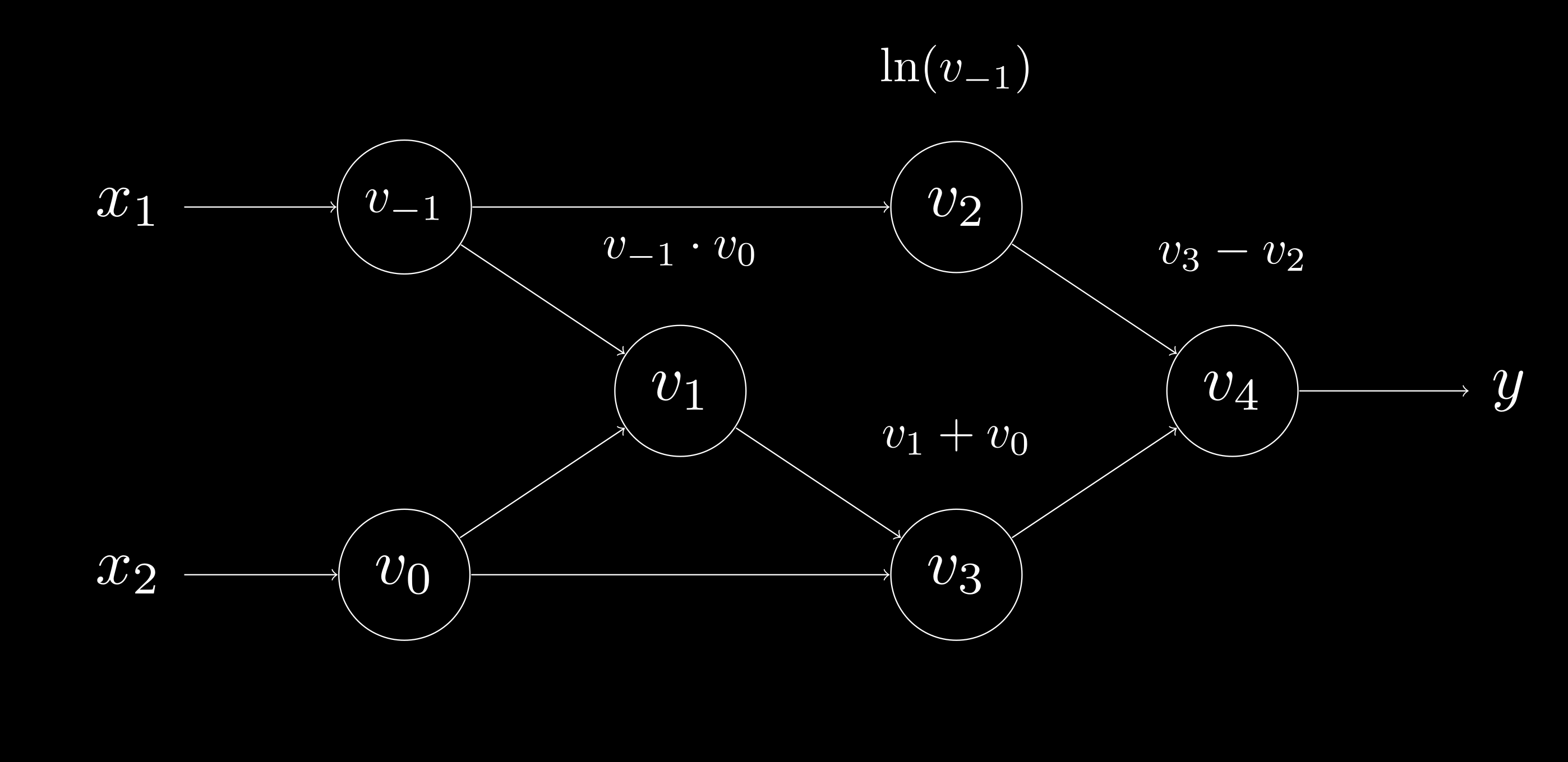
On top of the evaluation trace, we can use a Directed Acyclic Graph (DAG) as a data structure to algorithmically represent the evaluation trace. Nodes in the DAG represent input variables, intermediate variables, and output variables, while edges describe the computational hierarchy of input to output transformations. Finally, the graph must be directed and acyclic to ensure the correct flow of computation. In its entirety, this type of DAG is commonly known as the computational graph.

Computational Graph (eq. 6)

The introduction of these tools, both the evaluation trace and computational graph, are important for understanding and implementing AD—in particular, its two modes: forward and reverse mode.

Forward Mode AD

---

Forward mode AD adopts the principles we previously covered from the evaluation trace, but introduces the tangent, denoted $\dot{v_i}\backslash dot\{v\_i\}$, corresponding to a primal $v_{i}v\_i$. These tangents carry the partial derivative information of a primal w.r.t. a particular input variable of interest.

Referencing back to eq. 6, we'd have the following definition of tangents if we were interested in finding $\frac{\mathrm{\partial }y}{\mathrm{\partial }{x}_2}\backslash frac\{\backslash partial\{y\}\}\{\backslash partial\{x\_2\}\}$:

$$\dot{v_i}=\frac{\mathrm{\partial }{v}_i}{\mathrm{\partial }{x}_2}\backslash dot\{v\_i\}\; =\; \backslash frac\{\backslash partial\{v\_i\}\}\{\backslash partial\{x\_2\}\}$$

Continuing from this definition, we can build out the forward primal and forward tangent trace to compute $\frac{\mathrm{\partial }y}{\mathrm{\partial }{x}_2}\backslash frac\{\backslash partial\; y\}\{\backslash partial\; x\_2\}$ when $x_1=3x\_1\; =\; 3$, $x_2=-4x\_2\; =\; -4$, ${\dot{x}}_1=\frac{\mathrm{\partial }{x}_1}{\mathrm{\partial }{x}_2}=0\backslash dot\{x\}\_1\; =\; \backslash frac\{\backslash partial\; x\_1\}\{\backslash partial\; x\_2\}\; =\; 0$, and $\dot{x_2}=\frac{\mathrm{\partial }{x}_2}{\mathrm{\partial }{x}_2}=1\backslash dot\{x\_2\}\; =\; \backslash frac\{\backslash partial\; x\_2\}\{\backslash partial\; x\_2\}\; =\; 1$.

Forward Mode Trace (eq. 6)

This process is the essence of forward mode AD. At every elementary operation for a given function, compute intermediate variables (primals) by applying basic arithmetic operations, and in synchrony, compute their derivatives (tangents) by using what we know from Calculus.

With this approach, we can do more than just compute derivatives, but we can compute Jacobians. For a vector-valued function $f:{\mathbb{R}}^n\to {\mathbb{R}}^{m}f:\; \backslash R^n\; \backslash to\; \backslash R^m$, we choose a set of inputs $\mathbf{a}\in {\mathbb{R}}^n\backslash bold\{a\}\; \backslash in\; \backslash R^n$—where $\mathbf{x}=\mathbf{a}\backslash bold\{x\}\; =\; \backslash bold\{a\}$ and tangents $\dot{\mathbf{x}}={\mathbf{e}}_i\backslash bold\{\backslash dot\{x\}\}\; =\; \backslash bold\{e\}\_i$ for $i=1,\mathrm{.}\mathrm{.}\mathrm{.},ni=1,...,n$. Applying these inputs to our function in forward mode now generates the partial derivatives of the all output variables $y_{j}y\_j$ for $j=1,\mathrm{.}\mathrm{.}\mathrm{.},mj=1,...,m$ w.r.t. a single input variable $x_{i}x\_i$. Essentially, every forward pass in forward mode AD generates one column of the Jacobian—correlating to the partial derivatives of all outputs w.r.t. a single input.

Jacobian Matrix

Because the function $f:{\mathbb{R}}^n\to {\mathbb{R}}^{m}f:\; \backslash R^n\; \backslash to\; \backslash R^m$ has $nn$ inputs and one forward pass in forward mode generates a column of the Jacobian, it requires $O(n)O(n)$ evaluations to compute the full $m\times nm\; \backslash times\; n$ Jacobian matrix. If you don't recall from Linear Algebra, the full Jacobian represents the partial derivatives of all outputs w.r.t. to all inputs; for our purposes, the gradients we're trying to derive for optimization.

This feature generalizes to the Jacobian-vector product (JVP). JVPs are the dot-product between the Jacobian of a function $\mathbf{J}\in {\mathbb{R}}^{m\times n}\backslash bold\{J\}\; \backslash in\; \backslash R^\{m\; \backslash times\; n\}$, and a column vector $\mathbf{r}\in {\mathbb{R}}^n\backslash bold\{r\}\; \backslash in\; \backslash R^n$. The result of the dot product returns a $mm$-dimensional column vector encoding the change of the outputs when the inputs are perturbed. In better words, it describes the change in the outputs when the inputs are directionally nudged by $\mathbf{r}\backslash bold\{r\}$.

What makes this special, specifically in forward mode AD, is that we don't need to compute the full Jacobian. By choosing a set of inputs, and setting the perturbation vector $\mathbf{r}\backslash bold\{r\}$, one evaluation in forward mode for a function outputs the JVP without ever computing the entire Jacobian.

Jacobian-vector Product

Altogether, this makes forward mode AD practical in certain cases. To be specific, forward mode AD is effective when evaluating a function $f:{\mathbb{R}}^n\to {\mathbb{R}}^{m}f:\; \backslash R^\{n\}\; \backslash to\; \backslash R^m$ when $n\ll mn\; \backslash ll\; m$. For example, a function with one input and $mm$ outputs requires a single forward pass in this mode to compute its Jacobian. On the opposite end, a function with $nn$ inputs and one output ( $f:{\mathbb{R}}^n\to \mathbb{R}f:\; \backslash R^n\; \backslash to\; \backslash R$ ) requires $nn$ forward passes in forward mode to obtain its Jacobian.

This case is important to examine because, oftentimes, the parameters of a neural network represent ${\mathbb{R}}^n\backslash R^n$ while the scalar loss—caused by the model's parameters—represents $\mathbb{R}\backslash R$. Thus, if we were to use forward mode AD for gradient-based optimization, we'd be using it when it's suboptimal.

Wrapping up, forward mode AD is preferred over numeric and symbolic differentiation because it doesn't have issues like numerical instabilities or expression swell (see the Truncation vs. Round-off Error depiction and the Expression Swell example). But since it lacks the scalability we need for neural network optimization, we can pivot to AD's second mode, reverse mode.

Reverse Mode AD

---

Arriving at this point, we have reverse mode AD—alike forward mode, yet different methodically. We begin by defining adjoints ${\bar{v}}_i\backslash bar\{v\}\_i$ representing the partial derivative of an output $y_{j}y\_j$ w.r.t. an intermediate variable $v_{i}v\_i$ for a function $f:{\mathbb{R}}^n\to {\mathbb{R}}^{m}f:\; \backslash R^n\; \backslash to\; \backslash R^m$—where $i=1,\mathrm{.}\mathrm{.}\mathrm{.},ni\; =\; 1,...,n$ and $j=1,\mathrm{.}\mathrm{.}\mathrm{.},mj\; =\; 1,...,\; m$. We can formally define the adjoints as:

$${\bar{v}}_i=\frac{\mathrm{\partial }{y}_j}{\mathrm{\partial }{v}_i}\backslash bar\{v\}\_i\; =\; \backslash frac\{\backslash partial\; y\_j\}\{\backslash partial\; v\_i\}$$

In reverse mode AD, we perform the forward pass by applying elementary operations to compute intermediate variables, but during this stage, adjoints are not computed alongside their primal counterparts like we observed with the tangents in forward mode AD. Rather, any dependencies required for the derivative computation of ${\bar{v}}_i\backslash bar\{v\}\_i$ are stored in the computational graph.

Progressing, we use our familiarity with the derivatives of elementary operations, the chain rule, and the cached dependencies (from the forward pass) to compute the adjoints. Adjoints are computed in the order starting from an output variable and ending with all input variables that caused the output variable. This stage is commonly referred as the reverse pass. If you couldn't tell already, the "reverse" pass is what gives this mode of AD its name—in which derivatives are computed in a reversed fashion.

With intuition behind reverse mode AD, let's take a look at the reverse mode evaluation trace of
eq. 6 using the same values for the input variables from the Forward Mode Trace.

Reverse Mode Trace (eq. 6)

In this particular trace, we start with the adjoint $\bar{y}=\frac{\mathrm{\partial }y}{\mathrm{\partial }y}=1\backslash bar\{y\}\; =\; \backslash frac\{\backslash partial\; y\}\{\backslash partial\; y\}\; =\; 1$ and send it down to any of its dependencies (variables that caused it) by applying the derivative rules. Eventually, any input variable $xx$ that contributed to the output $yy$ will have its adjoint populated.

You might be confused by the computation of ${\bar{v}}_{-1}\backslash bar\{v\}\_\{-1\}$ and ${\bar{v}}_0\backslash bar\{v\}\_0$. This is slightly unintuitive in my opinion, but since their primals contribute to the output $yy$ through multiple paths—seen in the computation of $v_{2}v\_2$ and $v_{1}v\_1$—they'll each have two incoming derivatives. We don't discard any derivative information, favoring one over the other, because we'd lose how $x_{1}x\_1$ and $x_{2}x\_2$* influence $yy$. Instead, we accumulate their respective derivatives. In doing so, the total contribution of $x_{1}x\_1$ and $x_{2}x\_2$ are contained in their adjoints $\overline{x_1}\backslash bar\{x\_1\}$ and $\overline{x_2}\backslash bar\{x\_2\}$.

* Recall that $v_{-1}v\_\{-1\}$ and $v_{0}v\_0$ are just aliases for $x_{1}x\_1$ and $x_{2}x\_2$ respectively; the same is said for their adjoints.

As seen in forward mode, Jacobians can also be computed for vector-valued functions
$f:{\mathbb{R}}^n\to {\mathbb{R}}^{m}f:\; \backslash R^n\; \backslash to\; \backslash R^m$. By choosing inputs $\mathbf{a}\in {\mathbb{R}}^n\backslash bold\{a\}\; \backslash in\; \backslash R^n$, assigning $\mathbf{x}=\mathbf{a}\backslash bold\{x\; =\; a\}$, and setting $\bar{\mathbf{y}}={\mathbf{e}}_j\backslash bold\{\backslash bar\{y\}\}\; =\; \backslash bold\{e\}\_j$ for
$j=1,\mathrm{.}\mathrm{.}\mathrm{.},mj\; =\; 1,...,m$—each reverse pass generates the partial derivative of the $j\text{-th}j\backslash text\{-th\}$ output w.r.t. all input variables $x_{i}x\_i$ for $i=1,\mathrm{.}\mathrm{.}\mathrm{.},ni\; =\; 1,...,n$. Because there's $mm$ rows, and each reverse pass computes a row of the Jacobian, it would require $mm$ evaluations in reverse mode AD to achieve the full Jacobian of $ff$.

Expanding on above, we can compute the vector-Jacobian product (VJP). The VJP is the left multiply of a transposed row vector ${\mathbf{r}}^T\in {\mathbb{R}}^{1\times m}\backslash bold\{r\}^T\; \backslash in\; \backslash R^\{1\; \backslash times\; m\}$—often referred as the cotangent vector—and the Jacobian of a function $\mathbf{J}\in {\mathbb{R}}^{m\times n}\backslash bold\{J\}\; \backslash in\; \backslash R^\{m\; \backslash times\; n\}$. The computation of the VJP generates a $nn$-dimensional row vector containing the partial derivatives of an output w.r.t. all its inputs when perturbed by ${\mathbf{r}}^T\backslash bold\{r\}^T$.

Vector-Jacobian Product

Vector-Jacobian Product (Alt. Form)

VJPs tie directly into optimizing neural networks because we can represent $\mathbf{J}\backslash bold\{J\}$ as the partial derivatives of a model's outputs w.r.t. its inputs and ${\mathbf{r}}^T\backslash bold\{r\}^T$ as the partial derivatives of an objective loss function's output w.r.t. the model's outputs. Applying the VJP under this context produces the gradients needed for optimization. Also, like JVPs, VJPs don't require the full Jacobian of a function and can be computed in a single reverse pass.

Rounding off what we've discussed with reverse mode AD, it requires a single reverse pass to compute the gradients of an output w.r.t. all inputs and $mm$ reverse passes when computing such for $mm$ outputs. Because of these properties, reverse mode AD is best utilized when $n\gg mn\; \backslash gg\; m$. As a matter of fact, this makes reverse mode optimal for optimizing neural networks. It would only require one reverse pass to compute the gradients of a scalar producing loss function w.r.t. to the
$nn$-parameters of a model influencing it; recall the case of $f:{\mathbb{R}}^n\to \mathbb{R}f:\; \backslash R^n\; \backslash to\; \backslash R$.

Note: since dependencies for derivative computations must be stored in the computational graph, there's a memory complexity proportional to the number of operations for a function. This is a drawback, but doesn't undermine its practically for optimizing neural networks.

All things considered, reverse mode AD is clearly the best option for gradient-based optimization. We only need one reverse pass for one step of gradient descent, with the addition of added memory—an acceptable trade-off given we favor time over space.

Implementation

---

Having forward mode and reverse mode AD covered, we can delve into the implementation of the two in code. A couple of ways we might achieve this is via special-purpose compilers or source code transformation. Both implementations work, but are more involved than what's needed for a basic demonstration. Instead, we will opt for the operator overloading approach.

Operator overloading—in the context of AD—involves overriding the methods of operators for a custom type such that the functionality of AD is incorporated in them. You can think of this type as a user-defined class, struct, or object—depending on the language—with properties enabling AD. With the right implementation of operator overloading, any arithmetic operations applied on the AD enabled type(s) will allow for effortless derivations.

Python is a relatively simple language and supports operator overloading which is why we'll use it for our implementation of forward and reverse mode AD.

Forward Mode AD Implementation

class Variable:

    def __init__(self, primal, tangent):
        self.primal = primal
        self.tangent = tangent

    def __add__(self, other):
        primal = self.primal + other.primal
        tangent = self.tangent + other.tangent
        return Variable(primal, tangent)

    def __sub__(self, other):
        primal = self.primal - other.primal
        tangent = self.tangent - other.tangent
        return Variable(primal, tangent)

    def __mul__(self, other):
        primal = self.primal * other.primal
        tangent = self.tangent * other.primal + other.tangent * self.primal
        return Variable(primal, tangent)

    def __truediv__(self, other):
        primal = self.primal / other.primal
        tangent = (self.tangent / other.primal) + (
            -self.primal / other.primal**2
        ) * other.tangent
        return Variable(primal, tangent)

    def __repr__(self):
        return f"primal: {self.primal}, tangent: {self.tangent}"

Beginning with the Variable type (our AD type), we will take two arguments, primal and tangent, and initialize them as attributes for later use. Rather obvious, primal represents the primal used during the forward pass of an arithmetic operation. Likewise, tangent is the tangent used for the derivative computation during the forward pass of an arithmetic operation. For simplicity, both attributes will be scalars, but one can extend the functionality to operate on multi-dimensional arrays using numpy.

Moving on, we begin to overload the builtin arithmetic operators in python. In particular, we only overload* +, -, *, and /—correlating to __add__, __sub__, __mul__, and __truediv__ respectively. Just briefly, overloading these operators defines the behavior when (in the case of __add__) a + b is encountered—where a (self argument) is of type Variable and b (other argument) is some other type. For the sake of simplicity, b will always be of type Variable. As mentioned before, we can add more functionality by overloading more operators (e.g. __pow__ for a ** b), but I'm trying to keep things simple.

* __repr__ is also overloaded which dictates the behavior whenever repr(), print(), or str() is called on a Variable object. This is added just so we can represent Variable whenever we print it.

For each overloaded arithmetic operator, we implement the following procedure below.

Forward Mode AD Procedure:

1. Evaluate the operator with its operands (self and other).

2. Apply the derivative rules of Calculus and compute the partial derivative of the output w.r.t. each input.

3. Sum the derivatives together to get tangent—the derivative of the output w.r.t. to both inputs.

4. Create and return a new Variable object with the result of forward computation and the derived tangent.

Let's use __mul__—the multiplication of two numbers—to help us understand this procedure by breaking it down into each component.

Procedure for Multiply:

1. We evaluate the operator with its operands by computing self.primal * other.primal and then store the result in another variable primal.

2. We find the partial derivative of the output w.r.t. to each input by computing self.tangent * other.primal and other.tangent * self.primal.

3. Next, we sum the values from step 2 and store them in tangent. This is the derivative of the output w.r.t to both inputs.

4. Lastly, we return a new variable carrying the output of the arithmetic operation, and the associated tangent in return Variable(primal, tangent).

If operator overloading is implemented correctly on elementary arithmetic operations with well-defined derivatives, operations can be composed together to form differentiable composite functions. Down below, I've left some basic functions that test Variable's ability to help compute the evaluation of an expression and its derivative.

AD Computation in Forward Mode

def mul_add(a, b, c):
    return a * b + c * a

def div_sub(a, b, c):
    return a / b - c

a, b, c = Variable(25.0, 1.0), Variable(4.0, 0.0), Variable(-5.0, 0.0)
print(f"{a = }, {b = }, {c = }")
print(f"{mul_add(a, b, c) = }")
a.tangent, b.tangent, c.tangent = 0.0, 1.0, 0.0
print(f"{div_sub(a, b, c) = }")

a = primal: 25.0, tangent: 1.0, b = primal: 4.0, tangent: 0.0, c = primal: -5.0, tangent: 0.0
mul_add(a, b, c) = primal: -25.0, tangent: -1.0
div_sub(a, b, c) = primal: 11.25, tangent: -1.5625

AD Computation in Forward Mode: In the first function we compute $y=a^2\cdot (b+c)y\; =\; a^2\; \backslash cdot\; (b\; +\; c)$ and derive $\frac{\mathrm{\partial }y}{\mathrm{\partial }a}\backslash frac\{\backslash partial\; y\}\{\backslash partial\; a\}$. In the following function, we compute $y=\frac{a}{b}-cy\; =\; \backslash frac\{a\}\{b\}\; -\; c$ and derive $\frac{\mathrm{\partial }y}{\mathrm{\partial }b}\backslash frac\{\backslash partial\; y\}\{\backslash partial\; b\}$.

Reverse Mode AD Implementation

class Variable:

    def __init__(self, primal, adjoint=0.0):
        self.primal = primal
        self.adjoint = adjoint

    def backward(self, adjoint):
        self.adjoint += adjoint

    def __add__(self, other):
        variable = Variable(self.primal + other.primal)

        def backward(adjoint):
            variable.adjoint += adjoint
            self_adjoint = adjoint * 1.0
            other_adjoint = adjoint * 1.0
            self.backward(self_adjoint)
            other.backward(other_adjoint)

        variable.backward = backward
        return variable

    def __sub__(self, other):
        variable = Variable(self.primal - other.primal)

        def backward(adjoint):
            variable.adjoint += adjoint
            self_adjoint = adjoint * 1.0
            other_adjoint = adjoint * -1.0
            self.backward(self_adjoint)
            other.backward(other_adjoint)

        variable.backward = backward
        return variable

    def __mul__(self, other):
        variable = Variable(self.primal * other.primal)

        def backward(adjoint):
            variable.adjoint += adjoint
            self_adjoint = adjoint * other.primal
            other_adjoint = adjoint * self.primal
            self.backward(self_adjoint)
            other.backward(other_adjoint)

        variable.backward = backward
        return variable

    def __truediv__(self, other):
        variable = Variable(self.primal / other.primal)

        def backward(adjoint):
            variable.adjoint += adjoint
            self_adjoint = adjoint * (1.0 / other.primal)
            other_adjoint = adjoint * (-1.0 * self.primal / other.primal**2)
            self.backward(self_adjoint)
            other.backward(other_adjoint)

        variable.backward = backward
        return variable

    def __repr__(self) -> str:
        return f"primal: {self.primal}, adjoint: {self.adjoint}"

The reverse mode AD implementation is rather similar to the forward mode implementation—granted adjoint and tangent serve the same purpose. Where the two diverge is the fact we default adjoint to 0. This is because in reverse mode, we propagate derivatives from output to input then accumulate them; we don't know the derivative(s) to accumulate for a Variable at the time of its creation, so it gets set to zero for the time being.

Let's also touch on the default backward method for the Variable type. All this method does is take the adjoint argument, and accumulates it into the adjoint attribute of the Variable object invoking it. Essentially, its purpose is to accumulate the derivative for the leaf* Variables that don't have a custom backward method. This may not make sense at the moment, but as we explore the reverse mode AD implementation, its purpose will be clearer.

* Think of leaf Variables as the independent input variables $x_{i}x\_i$ that we discussed in the Automatic Differentiation section.

With enough background, let's look into the procedure to enable reverse mode AD for our Variable type.

Reverse Mode AD Procedure:

1. Create a Variable object holding the result of the operator and its operands.

2. Define a closure function backward that does the following:

   • Accepts an adjoint as an argument and accumulates it into the adjoint of the Variable object from 1.
   • Computes the partial derivative of the output w.r.t. to each input using the operator's derivative and the adjoint to chain incoming derivatives.
   • Calls backward() on each input with their respective derivatives (second bullet) to continue the reverse pass.

3. Return the resultant Variable object from 1. with its backward method overwritten with the closure function defined in 2.

To further our grasp, let's examine this procedure implemented in __truediv__—the floating-point division between two numbers.

Procedure for Division:

1. We create a new Variable with the result of the arithmetic operator applied with its operands in variable = Variable(self.primal / other.primal).

2. Moving to the next step, we create the closure function backward(adjoint) where we:

   • Accumulate the adjoint argument into variable by doing variable.adjoint += adjoint.

   • Compute the partial derivative for each input using the quotient rule and adjoint—to chain derivatives—by defining self_adjoint = adjoint * (1.0 / other.primal) and other_adjoint = adjoint * (-1.0 * self.primal / other.primal**2).

   • Continue the reverse pass on both inputs by calling self.backward(self_adjoint) and other.backward(other_adjoint).

3. Lastly, we bind the closure function and return the modified Variable object equipped for reverse mode derivation in variable.backward = backward and return variable.

Referencing back, this implementation is why we need the default backward method. Eventually, the derivatives will propagate to leaf Variables, and since they don't need to propagate derivatives themselves, we'd just accumulate their derivatives passed from backward when a closure function calls them.

Like before, the proper implementation of operator overloading on elementary arithmetic operations (with well-defined derivatives) enables the automatic differentiation of differentiable composite functions. Below is the same test code from the forward mode example, but using our reverse mode implementation instead.

AD Computation in Reverse Mode

def mul_add(a, b, c):
    return a * b + c * a

def div_sub(a, b, c):
    return a / b - c

a, b, c = Variable(25.0, 1.0), Variable(4.0, 0.0), Variable(-5.0, 0.0)

print(f"{a = }, {b = }, {c = }")
d = mul_add(a, b, c)
d.backward(1.0)
print(f"{d = }")
print(f"{a.adjoint = }, {b.adjoint = }, {c.adjoint = }")

a.adjoint, b.adjoint, c.adjoint = 0.0, 0.0, 0.0
e = div_sub(a, b, c)
e.backward(1.0)
print(f"{e = }")
print(f"{a.adjoint = }, {b.adjoint = }, {c.adjoint = }")

a = primal: 25.0, adjoint: 0.0, b = primal: 4.0, adjoint: 0.0, c = primal: -5.0, adjoint: 0.0
d = primal: -25.0, adjoint: 1.0
a.adjoint = -1.0, b.adjoint = 25.0, c.adjoint = 25.0
e = primal: 11.25, adjoint: 1.0
a.adjoint = 0.25, b.adjoint = -1.5625, c.adjoint = -1.0

AD Computation in Reverse Mode: the code follows the same functions from the forward mode implementation ( $y=a^2\cdot (b+c)y\; =\; a^2\; \backslash cdot\; (b\; +\; c)$ and $y=\frac{a}{b}-cy\; =\; \backslash frac\{a\}\{b\}\; -\; c$ ), but now we've computed the partial derivatives for all the inputs and not just one as seen in forward mode. Also, note that we zero the adjoints before we call div_sub. If we hadn't, we'd accumulate the partial derivatives from it with those computed from mul_add.

Autograd

---

Hinting at it a bit, this implementation draws inspiration from PyTorch's autograd API. If you've trained a model using their framework, you've probably encountered loss.backward() before. This method (at least to me) looked like some form of magic, but in reality it's automatically differentiating the loss w.r.t. a model's parameters using an approach similar to our's above. The only difference is that PyTorch's implementation is more advanced and extends its functionality beyond the basic arithmetic operators to make it a viable framework for ML research...unlike ours.

Amazed by the PyTorch framework, I decided to develop my own in nura. It's far from complete, but it's a fun project which shows how an autograd engine and ML framework can be built with just numpy. Its main capabilities provide reverse and forward mode AD functionalities, but it also includes the ability to create neural networks similar to the torch.nn interface in PyTorch. To give you more of an idea, below is a snippet showing how one can evaluate and compute the Jacobian of a function using forward mode AD.

import nura
from nura.autograd.functional import jacfwd

def fn(a, b, c):
    return a * b + c

a = nura.tensor([1.0, 2.0, 3.0, 4.0])
b = nura.tensor([5.0, 6.0, 7.0, 8.0])
c = nura.tensor(1.0)
r = nura.ones(4).double()

output, jacobian = jacfwd((a, b, c), fn, pos=1)
print(f"output:\n{output}\n\njacobian:\n{jacobian}")

output:
tensor([ 6. 13. 22. 33.]) dtype=double)

jacobian:
tensor([[1. 0. 0. 0.]
       [0. 2. 0. 0.]
       [0. 0. 3. 0.]
       [0. 0. 0. 4.]]) dtype=double)

Conclusion

---

In this blog, we unpacked the challenge of efficiently computing gradients to optimize neural networks. We found numerical and symbolic differentiation as potential solutions, but their issues led us to automatic differentiation. In AD, we learned how to leverage the evaluation trace and computational graph to compute partial derivatives in forward mode. However, we noticed the properties of reverse mode handled this task more efficiently when it came to neural networks and gradient descent. Lastly, we strengthened our understanding of AD by implementing and testing both modes with our Variable type in python.

In closing, I hope this blog not only highlights the practicality of AD for neural network optimization via gradient descent, but also how we can leverage mathematics and a system design thought process to solve challenging problems in the field of ML.

Links

---

Reference Material

• Automatic Differentiation (source paper)

• What is Automatic Differentiation (video)

• Automatic Differentiation lecture (video)

• Pytorch Autograd Explained (video)

• A Gentle Introduction to torch.autograd (blog)

• Numerical Differentiation w/ Finite Difference Derivatives (video)

Personal

• Github

• LinkedIn

• Gmail