What is a Transformer?


Motivation
As a kid, I grew fascinated by technology and the innovations it led to. One area of particular interest was the foundations of artificial intelligence (AI), and its subset, machine learning (ML). With this new passion, I learned about computer vision (CV) and how computers see by building convolutional neural networks (CNNs). I gained intuition of how autonomous vehicles navigated because I trained reinforcement learning (RL) models. Now, I’m motivated to uncover how computers model language because I stumbled across the “Attention Is All You Need” paper.
Diving deep into the paper, I was impressed by the groundwork it laid and the implications it held for the future of deep learning. The nuances the paper presented were transformative and pathed the way for powerful large language models (LLMs) like: GPT-2 & 3, BERT, XLNET, the coding companion GitHub Copilot, and the very famous ChatGPT. As I write this, LLMs have taken precedent in our workflows by reducing hours spent researching, helping us debug code, and sometimes doing our homework… Through these possibilities and my curiosity, I took on the challenge of building the architecture responsible for them: the Transformer.
Undertaking the task was pretty difficult, and refining my knowledge for the subject spanned across months, but building the original sequence-to-sequence Transformer granted me a deeper understanding of LLMs and their importance going forward in AI. In the end, I hope to not only show you how to build the Transformer, but also to give you the same passion this project gave me for your endeavors.
Prerequisites
Given this subject is relatively advanced, I assume you have some experience programming and that you have a basic understaninding of the technical aspects behind AI. Because we’ll be working with PyTorch, it’s recommended you have some background utilizing this python framework as well. Continuing, there’s a lot of concepts and terms we’ll cover; if you’re not familiar, I’ve left refreshers below to help you understand some of the topics we’ll discuss.
- Machine learning (ML)
- Neural networks (NN)
- Deep learning (DL)
- Natural language processing (NLP)
- Neural machine translation (NMT)
Transformer Explained
To begin, the Transformer is a deep neural network that learns the relationship of input sequences (source) and output sequences (target) for a variety of sequence to sequence tasks, such as language translation. It uses the hidden representations of tokens (embeddings), the positioning of tokens in a sequence (positional encodings), the contextual correlation of tokens with respect to one another (attention mechanism), non-linear relationships (position-wise feed-forward network), and some other deep learning techniques (e.g. normalization, regularization, etc.) to perform this task. This approach not only makes Transformers the state of the art (SOTA) architecture for NLP tasks, but also resolves some of the pitfalls of older NLP architectures such as RNNs.
Note: For future reference, I use ‘tokens’ and ‘words’ interchangeably, but the two do not share the same meaning. A token can be thought of as a word or sub-words (e.g. 'learning' is tokenized into the tokens 'learn' and 'ing'). If you are curious about what tokenization is, you can learn more from the huggingface nlp course.
Encoder-Decoder Architecture
In NMT, the Encoder-Decoder architecture is a common implementation for transforming input sequences into hidden representations for translation. Within the Transformer, the Encoder takes an input sequence of tokens xₙ, with length n, and encodes it into the hidden representation zₙ. Next, the Decoder takes the output of the Encoder zₙ and decodes it into a sequence of output tokens yₘ, with length m. This process is auto-regressive, so the Decoder predicts one token at a time from the information contextualized by the Encoder output zₙ and information it previously predicted yₘ₋₁.
 Transformer architecture (Encoder left and Decoder right)
Embeddings
Embeddings are an important part for converting sequences made up of tokens into hidden representations. To simply put it, embeddings take a sequence of words and map each word into a series of values that best describe the word. The values for each word are assigned by the embedding weights and these weights can change as the embedding layer learns the relationships between words within the entire vocabulary (more on embeddings from this article.
In the “Attention Is All You Need” paper, every token in sequences will be embedded into a vector of 512 values. (i.e. dₘ = 512). Moving forward, dₘ is a hyperparamter that defines the dimensions of the Transformer's hidden representations. In the actual paper it's referenced as dmodel, but I adopt my notation for simplicity sake. You'll see this hyperparameter reused throughout the Transformer which will make more sense as you progress through this blog.
import torch.nn as nn

class Embeddings(nn.Module):

    def __init__(self, vocab_size, dm, pad_id) -> None:
        super().__init__()
        self.embedding = nn.Embedding(vocab_size, dm, padding_idx=pad_id)

    def forward(self, x):
        # inshape: x - (batch_size, seq_len)

        # embed tokens to dm | shape: out - (batch_size, seq_len, dm)
        out = self.embedding(x)
        return out
Positional Encodings
Now that there’s a way to understand the meaning of tokens in input sequences, we must now relate them positionally to one another. This is important because we wouldn’t say “Star Wars is the greatest movie franchise of all time.” has the same meaning as “Wars greatest Stars the franchise movie of is greatest time all.”, so positional encodings are needed to capture the order of tokens in sequences.
Since the Transformer model doesn’t use recurrence found in prior architectures to positionally relate tokens, sinusoidal patterns (i.e. sine and cosine functions) are used to encode the positions of tokens within sequences.
 Positional encodings functions
The encodings are first created based on the maximum length of sequences and the hidden dimensions of the the model. Continuing, the equations above allows positions of tokens to be mapped through sinusoids. pos represents the position, or index, of the word in the tokenized text sequence, i represents the index of the hidden representation of the position, and d model is the hidden dimensions of the model; we previously stated dₘ = 512.
If the positions are plotted using the sine function, different positions will have different encodings due to the wavelike behavior of the function. Although, some tokens with different positions may get the same encodings because the sine wave repeats. To counteract this, i is used to output multiple sinusoids (frequencies) for a single position allowing unique encodings for each token in a sequence. Essentially, i creates alternating sine and cosine waves depending on whether its value is even or odd, allowing the model to "attend by relative positions" more easily during training (visuals and more granular explanation from this post).
When processing inputs, the positional encoder sums the embeddings and corresponding positional encodings to capture both the meaning, and order of tokens within sequences.
import torch
import torch.nn as nn
import numpy as np

class PositionalEncoder(nn.Module):

    def __init__(self, dm, maxlen, dropout=0.1, scale=True) -> None:
        super().__init__()
        self.dm = dm
        self.drop = nn.Dropout(dropout)
        self.scale = scale

        # shape: pos - (maxlen, 1) dim - (dm, )
        pos = torch.arange(maxlen).float().unsqueeze(1)
        dim = torch.arange(dm).float()

        # apply pos / (10000^2*i / dm) -> use sin for even indices & cosine for odd indices
        values = pos / torch.pow(1e4, 2 * torch.div(dim, 2, rounding_mode="floor") / dm)
        encodings = torch.where(dim.long() % 2 == 0, torch.sin(values), torch.cos(values))

        # reshape: encodings - (1, maxlen, dm)
        encodings = encodings.unsqueeze(0)

        # register encodings w/o grad
        self.register_buffer("pos_encodings", encodings)

    def forward(self, embeddings):
        # inshape: embeddings - (batch_size, seq_len, dm)

        # scale embeddings (if applicable)
        if self.scale:
            embeddings = embeddings * np.sqrt(self.dm)
        # sum embeddings w/ respective positonal encodings | shape: embeddings - (batch_size, seq_len, dm)
        seq_len = embeddings.size(1)
        embeddings = embeddings + self.pos_encodings[:, :seq_len]
        # drop neurons | out - (batch_size, seq_len, dm)
        out = self.drop(embeddings)
        return out
Note: It is common practice in the Transformer to not only scale the embeddings by the square root of the model’s hidden dimensions for normalization, but also to regularize them by dropping 10% of the values using a dropout (i.e. scale = sqrt(dₘ) and dropout = 0.1). The addition of these components aid the model's learning ability and prevents it from overfitting during training.
With embeddings and positional encodings explained, we can go further into the main sublayer that allows the Transformer to understand contextual information: the attention mechanism.
Attention
Attention is a mechanism that takes a query and key-value pairs, and applies weights to the values based on the similarities between the query and keys. In a sense, the attention mechanism allows the Transformer to learn how to contextualize sequences, but also how to ‘translate’ those contextualized sequences. In NMT, there are many different implementations of attention, but in the Transformer, scaled dot-product attention is used.
Scaled Dot-Product Attention
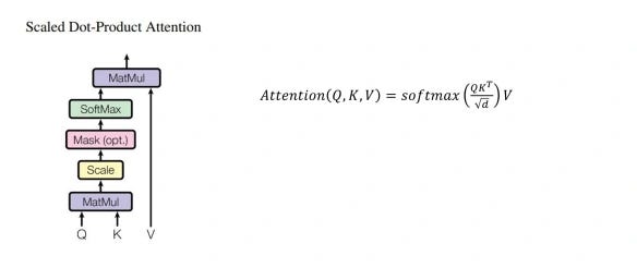 Scaled dot-product attention diagram and function
In scaled dot-product attention, we compute the dot product between the query (Q) and keys (K), both with dimensions dₖ. This yields the similarities between the query and the keys. Next, the similarities are scaled by the square root of the model’s hidden dimension; a step necessary to prevent diminishing gradients that can occur during back-propagation due to the application of softmax that follows this operation. After softmax is applied to the scaled similarities, we get the attention weights. Finally, we carry out a matrix multiplication between the attention weights and the values (V), which have dimensions dᵥ. The result of this step is the context vector of the passed sequence.
import torch
import torch.nn as nn
import numpy as np

class ScaledDotProductAttention(nn.Module):

    def __init__(self, dk, dropout=None) -> None:
        super().__init__()
        self.dk = dk
        self.drop = nn.Dropout(dropout)
        self.softmax = nn.Softmax(dim=-1)

    def forward(self, q, k, v, mask=None):
        # inputs are projected | shape: q - (batch_size, *n_head, q_len, dk) k - (batch_size, *n_head, k_len, dk)  v - (batch_size, *n_head, k_len, dv)

        # compute dot prod w/ q & k then scale | shape: similarities - (batch_size, *n_head, q_len, k_len)
        similarities = torch.matmul(q, k.transpose(-2, -1)) / np.sqrt(self.dk)

        # apply mask (if required)
        if mask is not None:
            mask = mask.unsqueeze(1) # for multi-head attention
            similarities = similarities.masked_fill(mask == 0,-1e9)

        # compute attention weights | shape: attention - (batch_size, *n_head, q_len, k_len)
        attention = self.softmax(similarities)
        # drop attention weights
        attention = self.drop(attention)

        # compute context given v | shape: context - (batch_size, *n_head, q_len, dv)
        context = torch.matmul(attention, v)
        return context, attention
Note: In my implementation, I employ a dropout layer to regularize the attention weights before they’re matrix multiplied with the values.
Scaled dot-product attention allows the Transformer to evaluate the importance of tokens with respect to one another in given sequence, while doing so in parallel. This parallel capability proved to be a substantial advantage for this architectural component since prior architectures were stuck with sequential processing. Somehow, the authors of the “Attention Is All You Need” paper found ways to leverage more performance from this component via multi-head attention.
Multi-Head Attention
 Multi-head attention diagram
Multi-head attention is a sublayer that performs multiple computations of scaled dot-product attention concurrently by splitting the query and key-value pairs into multiple attention heads. In this implementation, the query and keys, both having dimensions dₖ, as well as the values with dimensions dᵥ, are each projected h times where ‘h’ symbolizes the number of attention heads. The projections for the query and key-value pairs are created from three learnable weight matrices: Wq for the query, Wₖ for the keys, and Wᵥ for the values. The projections of the query and key-value pairs allows the Transformer to attend to multiple subspaces at varying positions.
Once projected and split into the attention heads, scaled dot-product attention is computed simultaneously between the query and key-value pairs within each head. Next, the resultant context vectors, which are split across multiple heads, are concatenated together to form a single context vector; which matches the dimensions of the model. Now unified, the context vector is projected using a distinct learnable weight matrix, represented as Wₒ. The result of this operation outputs the final context vector of the query and key-value pairs.
To simplify what’s happening underneath, multi-head attention lets the Transformer view different parts of sequences from different perspectives which increases the effectiveness of attention.
class MultiHeadAttention(nn.Module):

    def __init__(self, dm, dk, dv, nhead, bias=False, dropout=None) -> None:
        super().__init__()
        if dm % nhead != 0:
            raise ValueError("Embedding dimensions (dm) must be evenly divisble by number of heads (nhead)")
        self.dm = dm
        self.dk = dk
        self.dv = dv
        self.nhead = nhead
        self.wq = nn.Linear(dm, dk * nhead, bias=bias)
        self.wk = nn.Linear(dm, dk * nhead, bias=bias)
        self.wv = nn.Linear(dm, dv * nhead, bias=bias)
        self.wo = nn.Linear(dv * nhead, dm)
        self.scaled_dot_prod_attn = ScaledDotProductAttention(dk, dropout=dropout)

    def forward(self, q, k, v, mask=None):
        # inshape: q - (batch_size, q_len, dm) k & v - (batch_size, k_len, dm)
        batch_size, q_len, k_len = q.size(0), q.size(1), k.size(1)

        # linear projections into heads | shape: q - (batch_size, nhead, q_len, dk) k - (batch_size, nhead, k_len, dk) v - (batch_size, nhead, k_len, dv)
        q = self.wq(q).view(batch_size, q_len, self.nhead, self.dk).transpose(1, 2)
        k = self.wk(k).view(batch_size, k_len, self.nhead, self.dk).transpose(1, 2)
        v = self.wv(v).view(batch_size, k_len, self.nhead, self.dv).transpose(1, 2)

        # get context & attn weights | shape: attention - (batch_size, nhead, q_len, k_len) context - (batch_size, nhead, q_len, dv)
        context, attention = self.scaled_dot_prod_attn(q, k, v, mask=mask)

        # concat heads | shape: context - (batch_size, q_len, dm)
        context = context.transpose(1, 2).contiguous().view(batch_size, q_len, self.dm)

        # project context vector | shape: context - (batch_size, q_len, dm)
        context = self.wo(context)
        return context, attention
Note: The learnable weight matrices used to project the query and key-value pairs have no bias (i.e. bias = False).
Padding Masks and No-peak Subsequent Masks
You might’ve spotted the application of masks in our PyTorch implementation for computing scaled dot-product attention. Masks are crucial to the attention mechanism and play a role for two specific use cases:
- ensuring padded positions within sequences get ignored when computing attention.
- To prevent the Decoder from gaining an unfair advantage when predicting words during training.
Ignoring Padding
For parallel and efficient training, sequences are batched together where all sequences in the batch must have the same sequence length. Because not all sequences will have the exact same length in the training data, we pad sequences to the same length, allowing them to be batched together. Since padding applies zero contextual meaning to a sequence, we ignore the embedding values where there’s padding; which is exactly what the padding mask will do.
def generate_pad_mask(seq, pad_id):
    # inshape: seq - (batch_size, seq_len)

    # mark non-pad True & pad False
    mask = (seq != pad_id).unsqueeze(-2)
    # outshape: mask - (batch_size, 1, seq_len)
    return mask
When the mask is applied in scaled dot-product attention, positions where there’s pad, being labeled as False, get filled with an extremely large negative number (e.g. -1,000,000,000). Once softmax is applied to attain the attention weights, the values will be so insignificant that the gradient to update the weights will be negligible for padded positions. To simply put it, padded positions will be ignored for contextualizing the sequence.
No-Peak Subsequent Masks
No-peak subsequent masks are necessary during the training phase because they ensure the Decoder doesn’t attend to subsequent positions of sequences, but rather attends to positions it has already predicted within sequences. In layman’s terms, it makes sure the Decoder learns to predict each word successively (i.e. one by one) from the words it’s already predicted in a given sentence, instead of looking ahead to predict a word in the same sentence.
This is achieved by making a l x l matrix where l is the length of the sequence. The rows of the matrix represent the positions of the sequence that the Decoder can attend to at a ‘time-step’ and the columns represent the position of a token in the sequence. Positions labeled as True can be attended to, while positions marked as False cannot.
import torch

def generate_nopeak_pad_mask(trg, pad_id):
    # inshape: trg - (batch_size, trg_len)

    # create pad mask (True = no pad False = pad) | shape: trg_mask - (batch_size, 1, trg_len)
    trg_mask = generate_pad_mask(trg, pad_id)
    # create subsequent mask | shape: trg_nopeak_mask - (1, trg_len, trg_len)
    trg_len = trg.size(1)
    trg_nopeak_mask = torch.triu(torch.ones((1, trg_len, trg_len)) == 1)
    trg_nopeak_mask = trg_nopeak_mask.transpose(1, 2)
    # combine pad & subsequent mask shape
    trg_mask = trg_mask & trg_nopeak_mask
    # outshape: trg_mask - (batch_size, trg_len, trg_len)
    return trg_mask
Because padding rules still apply, the no-peak subsequent mask is combined (logically anded) with a corresponding padding mask to keep positions where there’s pad as False, regardless of whether the Decoder can attend to that position or not. From there, the same principle follows when softmax is applied, essentially negating attention to subsequent and padded positions within the Decoder.
 Example tensor of tokenized sequence (pad token id = 0)
 Padding mask for example tensor
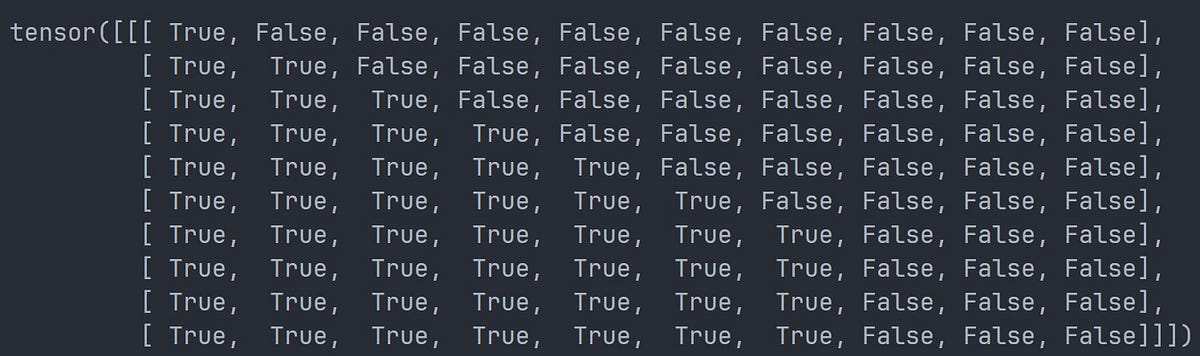 No-peak subsequent mask for example tensor
def generate_masks(src, trg, pad_id):
    # inshape: src - (batch_size, src_len) trg - (batch_size, trg_len)

    # create pad mask for src (True = no pad False = pad)
    src_mask = generate_pad_mask(src, pad_id)
    # generate pad nopeak mask for trg
    trg_mask = generate_nopeak_pad_mask(trg, pad_id)
    # outshape: src_mask - (batch_size, 1, src_len) trg_mask - (batch_size, trg_len, trg_len)
    return src_mask, trg_mask
Note: This snippet generates the required masks for both source and target sequences.
Position-wise Feed-forward Network
With most of the dirty work out the way, we can explore the position-wise feed-forward network. This sublayer is pivotable to furthering the learning capabilities of the Transformer.
 Position-wise feed-forward network function
The feed-forward network consists of two learnable weight matrices, W₁ and W₂, having a single ReLU activation in between. The dimensions of both matrices are defined by the model’s hidden dimensions and the specified dimensions of the network. Using the parameters from the “Attention Is All You Need” paper, the dimensions for the matrices are 512x2048 and 2048x512 respectively (i.e. dff = 2048).
The position-wise feed-forward network is essential to both the Encoder and Decoder blocks because it parameterizes attention modules. Without it, the context vectors passed to attention modules in subsequent layers would just be ‘re-averaged’, hampering the model’s ability to learn. Thus, its inclusion is necessary to allow more model functionality for learning complex patterns within the data (more about its implementation here).
import torch.nn as nn

class FeedForwardNetwork(nn.Module):

    def __init__(self, dm, dff, dropout=0.1) -> None:
        super().__init__()
        self.w1 = nn.Linear(dm, dff)
        self.w2 = nn.Linear(dff, dm)
        self.relu = nn.ReLU(inplace=False)
        self.drop = nn.Dropout(dropout)

    def forward(self, x):
        # inshape: x - (batch_size, seq_len, dm)

        # first linear transform with ReLU | shape: x - (batch_size, seq_len, dff)
        x = self.relu(self.w1(x))
        # drop neurons
        x = self.drop(x)
        # second linear transform | shape: out - (batch_size, seq_len, dm)
        out = self.w2(x)
        return out
Note: In my implementation I drop neurons before the second linear transformation to help with generalization and to reduce the chances of the network overfitting during training.
Layer Normalization
 Layer normalization formula via PyTorch
Last, but certainly not least, we have the layer normalization module (LayerNorm). Layer normalization is a technique used to normalize input's features from their mean and variance. During training, the layer normalization module uses gamma (γ) to scale, then beta (β) to shift the mean and variance of the features. Both gamma and beta are learnable parameters that may adjust as the module tries to stabilize the mean and variance. In the Transformer, the features being normalized are the varying hidden representations of tokenized sequences.
Layer normalization is incorporated in the Encoder and Decoder blocks for a variety of benefits. For one, it stabilizes gradients during training, which improves learning performance. It also makes convergence faster, causing an overall reduction in training time. Lastly, its presence may introduce better generalization during inference (here's a research paper delving into layer normalization for further understanding).
import torch
import torch.nn as nn

class Norm(nn.Module):

    def __init__(self, dm, eps=1e-6):
        super().__init__()
        self.gamma = nn.Parameter(torch.ones(dm))
        self.beta = nn.Parameter(torch.zeros(dm))
        self.eps = eps

    def forward(self, x: torch.Tensor):
        # inshape: x - (batch_size, seq_len, dm)

        # calc mean & variance (along dm)
        mean = x.mean(dim=-1, keepdim=True)
        var = x.var(dim=-1, unbiased=True, keepdim=True)
        # normalize, scale & shift | shape: out - (batch_size, seq_len, dm)
        norm = (x - mean) / torch.sqrt(var + self.eps)
        out = norm * self.gamma + self.beta
        return out
With all sublayers and modules described, we can create both the Encoder and Decoder.
Encoder Block
 Encoder block
In the “Attention Is All You Need” paper, the Encoder uses a multitude of components to function effectively. It’s main components are the multi-head attention and position-wise feed-forward network sublayers. On top of that, dropout, residual connections, and layer normalization is used to generate the final output of a sublayer.
Residual Connections
In the Transformer, all sublayers have an output shape identical to the dimensions of the model (dₘ = 512) which is intended to allow for residual connections. Residual connections are a key technique found in both the Encoder and Decoder blocks of the Transformer. They function as shortcuts for gradients between sublayers, preventing information from being lost during back-propagation. Since summation is a linear operation, gradients passing through residual connections will be unimpeded during back-propagation, even if some sublayers produce small gradients. Residual connections also serve to keep information consistent with the original inputs of sublayers. In multi-head attention, inputs are arbitrarily permuted which alters their original representation. Residual connections, pretty much, help sublayers ‘remember’ what their original inputs were. This ensures sublayer ouputs computed genuinely come from their original inputs and not from permuted alterations (further explanation).
Dropout
Dropout works by ignoring a fraction of inputs (i.e. setting their value to zero), meaning the model is forced to learn different representations of inputs independently. This regularization can make the model less prone to overfitting, and increase its robustness when generalizing to unseen inputs during inference (you can find out more about dropout from this research paper).
Sublayer Output
Residual connections and dropout are used to generate the final output of a sublayer. The function that describes this output before it’s passed to another can be defined by the pseudocode below:
output = LayerNorm(x + dropout(Sublayer(x)))
Pivoting back to the Encoder block, an input sequence (source) is embedded then positionally encoded. Following that, the result is passed to the multi-head attention sublayer where the context vector is computed. Dropout is then applied to the context vector, at which it is then summed with the original input of the multi-head attention sublayer via a residual connection. Lastly, the sum is normalized and passed as a new input for the position-wise feed-forward network.
For the position-wise feed-forward network, the same process is repeated, except the input is passed through the feed-forward network instead of the multi-head attention sublayer. This generates the final output of the Encoder block, which will later be used as an input in the Decoder block for Encoder-Decoder attention.
import torch.nn as nn
from embedding import Embeddings
from pos_encoder import PositionalEncoder
from attention import MultiHeadAttention
from norm import Norm
from feedforward import FeedForwardNetwork

class EncoderLayer(nn.Module):

    def __init__(self, dm, dk, dv, nhead, dff, bias=False, dropout=0.1, eps=1e-6) -> None:
        super().__init__()
        self.multihead = MultiHeadAttention(dm, dk, dv, nhead, bias=bias, dropout=dropout)
        self.feedforward = FeedForwardNetwork(dm, dff, dropout=dropout)
        self.norm1 = Norm(dm, eps=eps)
        self.norm2 = Norm(dm, eps=eps)
        self.drop1 = nn.Dropout(dropout)
        self.drop2 = nn.Dropout(dropout)

    def forward(self, src, src_mask=None):
        # inshape: src - (batch_size, src_len, dm)

        # get context | shape - x_out (batch_size, src_len, dm)
        x = src
        x_out, attn = self.multihead(x, x, x, mask=src_mask)
        # drop neurons
        x_out = self.drop1(x_out)
        # add & norm (residual connections) | shape: x - (batch_size, src_len, dm)
        x = self.norm1(x + x_out)

        # linear transforms | shape: x_out (batch_size, src_len, dm)
        x_out = self.feedforward(x)
        # drop neurons
        x_out = self.drop2(x_out)
        # add & norm (residual connections) | shape: out - (batch_size, src_len, dm)
        out = self.norm2(x + x_out)
        return out, attn

class Encoder(nn.Module):

    def __init__(self, vocab_size, maxlen, pad_id, dm, dk, dv, nhead, dff, layers=6, bias=False,
                 dropout=0.1, eps=1e-6, scale=True) -> None:
        super().__init__()
        self.embeddings = Embeddings(vocab_size, dm, pad_id)
        self.pos_encodings = PositionalEncoder(dm, maxlen, dropout=dropout, scale=scale)
        self.stack = nn.ModuleList([EncoderLayer(dm, dk, dv, nhead, dff, bias=bias, dropout=dropout, eps=eps)
                                    for l in range(layers)])

    def forward(self, src, src_mask=None):
        # inshape: src - (batch_size, src_len, dm) src_mask - (batch_size, 1, src_len)

        # embeddings + positional encodings | shape: x - (batch_size, src_len, dm)
        x = self.embeddings(src)
        x = self.pos_encodings(x)
        # pass src through stack of encoders (out of layer is in for next)
        for encoder in self.stack:
            x, attn = encoder(x, src_mask=src_mask)
        # shape: out - (batch_size, src_len, dm)
        out = x
        return out, attn
Note: Encoder blocks can be stacked multiple times where the output of a previous block is the input for the next block. The culmination, or in better words, the stacking of these blocks along with source embeddings and positional encodings, are the entirety of the Encoder. In the “Attention Is All You Need” paper, the base model has a stack of six (i.e. N = 6).
Decoder Block
 Decoder block
The Decoder block is quite similar to the Encoder block because it embeds and positionally encodes its inputs, uses the same sublayer output equation (see Residual Connections and Dropout section), and uses a position-wise feed-forward network as its final sublayer. However, it employs masked multi-head attention, followed by Encoder-Decoder attention as we mentioned previously.
Masked multi-head attention is similar to multi-head attention found in the Encoder block. The difference is it applies a no-peak subsequent mask (see Padding Masks and No-peak Subsequent Masks section) to prevent the Decoder from prematurely predicting tokens, or ‘cheating’, when learning to generate the output sequence (target).
When masked multi-head attention is computed, the context vector is passed to the next multi-head attention sublayer for Encoder-Decoder attention. In this instance of it, the context vector generated from masked multi-head attention serves as the query, while the output from the Encoder is utilized for key-value pairs. This step teaches the model how to ‘translate’ a source sequence to a target sequence. Finalizing, the context vector computed from Encoder-Decoder attention is passed through the position-wise feed-forward network, which creates the final output of the Decoder block.
import torch.nn as nn
from embedding import Embeddings
from pos_encoder import PositionalEncoder
from attention import MultiHeadAttention
from norm import Norm
from feedforward import FeedForwardNetwork

class DecoderLayer(nn.Module):

    def __init__(self, dm, dk, dv, nhead, dff, bias=False, dropout=0.1, eps=1e-6) -> None:
        super().__init__()
        self.maskmultihead = MultiHeadAttention(dm, dk, dv, nhead, bias=bias, dropout=dropout)
        self.multihead = MultiHeadAttention(dm, dk, dv, nhead, bias=bias, dropout=dropout)
        self.feedforward = FeedForwardNetwork(dm, dff, dropout=dropout)
        self.norm1 = Norm(dm, eps=eps)
        self.norm2 = Norm(dm, eps=eps)
        self.norm3 = Norm(dm, eps=eps)
        self.drop1 = nn.Dropout(dropout)
        self.drop2 = nn.Dropout(dropout)
        self.drop3 = nn.Dropout(dropout)

    def forward(self, src, trg, src_mask=None, trg_mask=None):
        # inshape: src - (batch_size src_len, dm) trg - (batch_size, trg_len, dm) \
        # src_mask - (batch_size, 1 src_len) trg_mask - (batch_size trg_len, trg_len)/(batch_size, 1 , trg_len)

        # calc masked context | shape: x_out - (batch_size, trg_len, dm)
        x = trg
        x_out, attn1 = self.maskmultihead(x, x, x, mask=trg_mask)
        # drop neurons
        x_out = self.drop1(x_out)
        # add & norm (residual connections) | shape: x - (batch_size, trg_len, dm)
        x = self.norm1(x + x_out)

        # calc context | shape: x_out - (batch_size, trg_len, dm)
        x_out, attn2 = self.multihead(x, src, src, mask=src_mask)
        # drop neurons
        x_out = self.drop2(x_out)
        # add & norm (residual connections) | shape: x - (batch_size, trg_len, dm)
        x = self.norm2(x + x_out)

        # calc linear transforms | shape: x_out - (batch_size, trg_len, dm)
        x_out = self.feedforward(x)
        # drop neurons
        x_out = self.drop3(x_out)
        # add & norm (residual connections) | shape: out - (batch_size, trg_len, dm)
        out = self.norm3(x + x_out)
        return out, attn1, attn2

class Decoder(nn.Module):

    def __init__(self, vocab_size, maxlen, pad_id, dm, dk, dv, nhead, dff, layers=6, bias=False,
                 dropout=0.1, eps=1e-6, scale=True) -> None:
        super().__init__()
        self.embeddings = Embeddings(vocab_size, dm, pad_id)
        self.pos_encodings = PositionalEncoder(dm, maxlen, dropout=dropout, scale=scale)
        self.stack = nn.ModuleList([DecoderLayer(dm, dk, dv, nhead, dff, bias=bias, dropout=dropout, eps=eps)
                                    for l in range(layers)])

    def forward(self, src, trg, src_mask=None, trg_mask=None):
        # inshape: src - (batch_size, src_len, dm) trg - (batch_size, trg_len, dm)

        # embeddings + positional encodings | shape: x - (batch_size, trg_len, dm)
        x = self.embeddings(trg)
        x = self.pos_encodings(x)
        # pass src & trg through stack of decoders (out of layer is in for next)
        for decoder in self.stack:
            x, attn1, attn2 = decoder(src, x, src_mask=src_mask, trg_mask=trg_mask)
        out = x
        return out, attn1, attn2
Note: Similar to Encoder blocks, Decoder blocks can be stacked, as well as paired with target embeddings and positional encodings to form the entirety of the Decoder. The original paper uses a stack of N = 6.
Now, there’s really not much to do with the output of the Decoder because it’s just the final hidden representation of it. Since we’re aiming to produce a vector where each position contains a list of probabilities for each word in the target vocabulary, the hidden representation is transformed.
Linear Transformation and Softmax
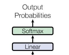 Linear transformation and softmax application
Linear Transformation
First, the Decoder output needs to be transformed from the continuous vector space of the model’s dimensions, to a representation of the target vocabulary. This can be achieved through the addition of a learnable linear layer, which has both the dimensions of the model and the number of tokens within the target vocabulary (i.e. dₘ x Vₜ, where Vₜ is the number of tokens in the target vocabulary).
Softmax
The next step is to create a probability distribution for each position in the sequence over the target vocabulary. This is easily achieved by computing softmax over the transformed vector along the dimension of the target vocabulary. Once it’s applied, it produces a sequence where each position corresponds to a list of probabilities for each word in the target vocabulary, a.k.a the predicted output token probabilities.
Putting it all together
With the hidden details and intricacies discussed, we can finally begin to place each piece of the puzzle together to build a Transformer.
import torch.nn as nn
from encoder import Encoder
from decoder import Decoder

class Transformer(nn.Module):

    def __init__(self, vocab_enc, vocab_dec, maxlen, pad_id, dm=512, dk=64, dv=64, nhead=8, layers=6,
                dff=2048, bias=False, dropout=0.1, eps=1e-6, scale=True) -> None:
        super().__init__()
        self.encoder = Encoder(vocab_enc, maxlen, pad_id, dm, dk, dv, nhead, dff,
                        layers=layers, bias=bias, dropout=dropout, eps=eps, scale=scale)
        self.decoder = Decoder(vocab_dec, maxlen, pad_id, dm, dk, dv, nhead, dff,
                        layers=layers, bias=bias, dropout=dropout, eps=eps, scale=scale)
        self.linear = nn.Linear(dm, vocab_dec)
        self.maxlen = maxlen
        self.pad_id = pad_id
        self.apply(xavier_init)

    def forward(self, src, trg, src_mask=None, trg_mask=None):
        # inshape: src - (batch_size, src_len) trg - (batch_size, trg_len)\
        # src_mask - (batch_size, 1, src_len) trg_mask - (batch_size, 1, trg_len, trg_len)

        # encode embeddings | shape: e_out - (batch_size, src_len, dm)
        e_out, attn = self.encoder(src, src_mask=src_mask)

        # decode embeddings | shape: d_out - (batch_size, trg_len, dm)
        d_out, attn, attn = self.decoder(e_out, trg, src_mask=src_mask, trg_mask=trg_mask)
        # linear transform decoder output | shape: out - (batch_size, trg_len, vocab_size)
        out = self.linear(d_out)
        return out

def xavier_init(module):
    if hasattr(module, "weight") and module.weight.dim() > 1:
        init.xavier_uniform_(module.weight.data)
Note: I’d like to point out, there’s no application of softmax after the Decoder output is transformed in our code. The reason is because the loss function used for training the Transformer, cross-entropy loss, applies softmax for you when computing loss in PyTorch. In addition, Xavier weight initialization is used to deter vanishing and exploding gradients, as well as give the model a good starting point to converge during training (further intuition about weight initialization can be found from this article).
Training
There’s nothing we can really do with the Transformer unless we train it on some data to do some translating. Below, is a general training function that takes your Transformer and trains it over a certain number of epochs using a custom Pytorch DataLoader, Optimizer, and optionally using a desired device (e.g. ‘cuda’ for parallel GPU computation).
import numpy as np
import torch.nn as nn
from utils.functional import generate_masks

def train(dataloader, model, optimizer, epochs=1000, device=None):
    # setup
    model.train()
    m = len(dataloader)
    cross_entropy = nn.CrossEntropyLoss(ignore_index=model.pad_id)
    losses = []

    # train over epochs
    print("Training Started")
    for epoch in range(epochs):
        accum_loss = 0 # reset accumulative loss
        for inputs, labels in dataloader:
            # get src & trg
            src, trg, out = inputs, labels[:, :-1], labels[:, 1:] # shape: src - (batch_size, src_len) trg & out - (batch_size, trg_len)
            src, trg, out = src.long(), trg.long(), out.long()
            # generate the masks
            src_mask, trg_mask = generate_masks(src, trg, model.pad_id)
            # move to device
            src, trg, out = src.to(device), trg.to(device), out.to(device)
            src_mask, trg_mask = src_mask.to(device), trg_mask.to(device)

            # zero the grad
            optimizer.zero_grad()
            # get pred & reshape outputs
            pred = model(src, trg, src_mask=src_mask, trg_mask=trg_mask) # shape: pred - (batch_size, seq_len, vocab_size)
            pred, out = pred.contiguous().view(-1, pred.size(-1)), out.contiguous().view(-1) # shape: pred - (batch_size * seq_len, vocab_size) out - (batch_size * seq_len)
            # calc grad & update model params
            loss = cross_entropy(pred, out)
            loss.backward()
            optimizer.step()
            # accumulate loss over time
            accum_loss += loss.item()

        # get epoch loss & keep track
        epoch_loss = accum_loss / m
        losses.append(epoch_loss)
        print(f"Epoch {epoch + 1} Complete | Loss: {epoch_loss:.4f}")

    # calc avg train loss
    loss = np.mean(losses).item()
    print(f"Training Complete | Average Loss: {loss:.4f}")
    return loss
Experiment
For my experiment, I trained the Transformer to perform English-to-German language translation. I trained and evaluated the model using the Multi30k dataset from torchtext version 0.4.0. For the configurations and hyper-parameters, I replicated the setup found in the base model of the “Attention Is All You Need” paper. I employ the same Adam optimizer, having an initial learning rate of 0.00001 (i.e. lr = 1e-5), with beta₁ = 0.9 and beta₂ = 0.98. I also include a scheduler that reduces the learning rate by 10% if the test loss plateaus for 10 epochs. Lastly, I use beam search with a beam width of 3 to decode tokens during inference.
There’s a multitude of other modules, tools, and hyper-parameters I use to both aid the model during training and view its performance. If interested, you can see my full implementation found in my GitHub repository.
Results
After training the model over 1000 epochs on Nvidia A10 GPUs from Lambda Cloud, I was able to get exceptional performance compared to the base Transformer found in the original “Attention Is All You Need” paper.
 Training snippet of the Transformer model
For my model, the average training loss over the Multi30k dataset was 1.2493, the average testing loss was 2.5804, and the best BLEU (Bilingual Evaluation Understudy) score was 25.7. This result was a delta of 0.1 compared to the result of the Transformer evaluated on a similar task outlined in “Attention Is All You Need” paper (25.8 to be specific).
 Metric performance of the Transformer after training (train loss in red, test loss in blue)
Conclusion
We’ve not only walked through the Transformer model step-by-step, but we’ve built one using PyTorch, and we were succesful in training the model to achieve respectable performance when evaluated over an English-to-German translation dataset.
Arriving at this point, I hope I was able to help you process the complexity of the Transformer, while shedding light on its features that make it a viable architecture for building LLMs. With this work complete, I’d like to thank you for taking consideration into this article and for future work, I plan to dive deeper into Decoder-only Transformer models, most notoriously found in ChatGPT.
Stay tuned…