ESMBind (ESMB): Low Rank Adaptation of ESM-2 for Protein Binding Site Prediction


 This image was obtained from the Metagenomic Atlas.
TLDR: LoRA applied to the protein language model ESM-2 is an effective and important finetuning and regularization strategy that appears to show comparable performance to SOTA structural models for the task of predicting binding residues in protein sequences on our train/test split. However, due to things such as sequence similarity this may be misleading and further cleaning of the data is required. The model predicts binding residues from single protein sequences alone and does not require MSA or structural information. Read on to better understand how to finetune a pLM with LoRA, complete with a code example for finetuning your own pLM LoRA and running inference on your favorite protein sequences.
Protein Language Models (pLMs) like ESM-2 are transformers, like their Large Language Model (LLM) counterparts, but trained on protein sequences rather than natural language texts. Each protein sequence is made up of 20 standard amino acids, and sometimes a few nonstandard amino acids as well. Often, as is the case with ESM-2 models, each amino acid, represented by a single letter, is treated as a token. So a protein sequence made up of 200 amino acids would have 200 tokens to be tokenized by the pLM. The pLM has all of the usual architecture of a transformer including the query, key, and value weight matrices , , and , and it represents each amino acid token as query, key, and value vectors when computing attention. Protein language models like ESM-2 are trained using a masked langauge modeling objective, and learn to predict masked amino acids. They have been shown to effectively predict protein 3D structures more accurately than AlphaFold2 and provide atomically accurate and fast predictions from single protein sequences. For more information on the base models that we used, see here, and here.
In this article, we are going to discuss applying a popular parameter efficient finetuning strategy known as Low Rank Adaptation, or LoRA. LoRAs have become quite popular in the LLM community and in the Stable Diffusion community, but they can also be used for finetuning protein language models as well! In fact, they have proven to be very useful as a regularization tool and have significantly reduced problematic overfitting when finetuning pLMs, which is quite an obstacle for proteins due to something known as protein homologues and the presence of highly similar sequences in the datasets.
What is... a LoRA?
Low Rank Adaptations are a parameter efficient fine-tuning strategy which are implemented in Hugging Face's PEFT library. For a conceptual guide to LoRA see here.
In the realm of deep learning, the concept of Low Rank Adaptations (LoRAs) was first introduced by Hu et. al.. These LoRAs provide an efficient alternative to the traditional finetuning of neural networks. The process begins by freezing the pre-existing weights of a layer in the neural network. For instance, in the context of a transformer's attention mechanism, this could involve freezing the weights of the query, key, or value matrices , , or .
Following this, a LoRA layer is introduced to one or more of these pre-trained weight matrices. If we consider to be a frozen weight matrix, the LoRA layer would take the form of , wherein constitutes the LoRA. Typically, these are low-rank decompositions, with and , where the original weight matrix is . It is common for to be significantly less than .
The application of LoRAs only provides significant benefits when is much smaller than the input and output dimension. We can opt for a small and implement a LoRA in lieu of conventional fine-tuning. Empirical evidence suggests that in many cases, selecting or is more than sufficient—even for large weight matrices in LLMs such as the query, key, and value matrices of a transformer's attention mechanism. In Stable Diffusion, the ranks in the LoRAs trained by the community are often much higher, but it is unclear how necessary this really is. Perhaps counter to our intuition, lower rank is often better, especially for regularization.
Let's now explore a scenario where the application of a LoRA does not yield any substantial benefits in terms of reducing the number of parameters:
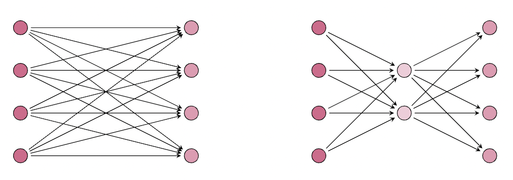
Here, we see that the number of parameters for the LoRA layer is the same as the original layer , where we have parameters for the LoRA (on the right), and parameters for the original frozen weight matrix (on the left). Next, let's look at an example that gives us % the parameters of the frozen weight matrix:
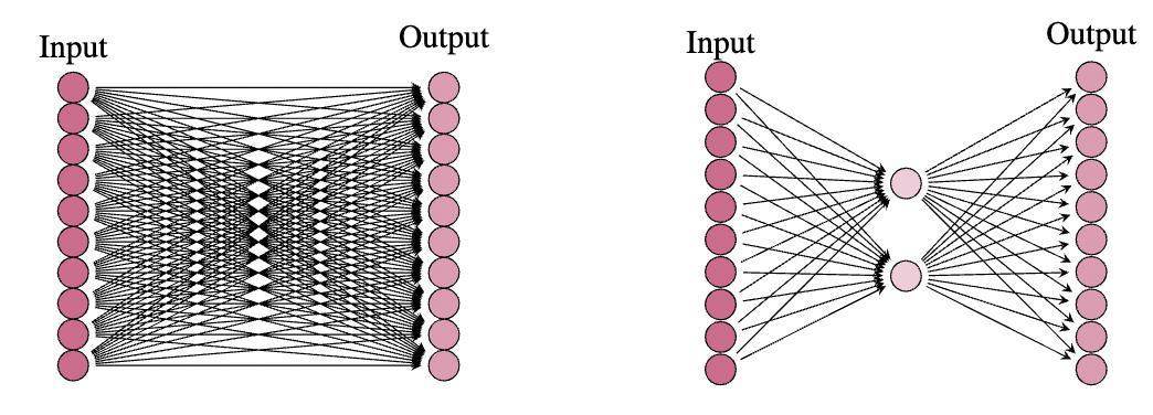
Here we see the original (frozen) weight matrix has parameters, and the LoRA has only parameters. In most cases, we have that the rank (this is the number of neurons in the middle layer of the LoRA) of the frozen matrix is much smaller than the input and output dimensions, and there is in fact a drastic reduction in parameter count. As an example, we might have an input and output dimension of say , in which case the weight matrix has parameters. However, the rank of this matrix is very often much lower than . In practice, it was shown that choosing for the query, key, and value matrices is often more than sufficient for a LoRA as the middle dimension. In this case, we would get parameters in the LoRA, which is less than one tenth the original parameter count. Once we have such a LoRA in place, we can train it on some downstream task, and then add the LoRA weight matrix to the original (frozen) weight matrix to obtain a model that performs well on this new task.
Importantly, LoRAs can help with issues such as overfitting, which can be a significant issue when learning on protein sequences. This, along with the parameter efficiency and a need to train larger models is why we decided to adopt LoRA as a fine-tuning strategy. Moreover, the simplicity of using a LoRA for parameter efficient fine tuning using the Hugging Face PEFT library makes it an attractive option. It also became clear early on that performance can actually increase with the use of LoRA, thus providing further motivation to adopt it as a strategy.
Overfitting and Regularization with LoRA
We first began by vanilla finetuning the smallest ESM-2 model on ~209K protein sequences. The data was eventually sorted by family according to UniProt to help with overfitting and overly optimistic results on generalization capabilities, but initially we didn't consider things like sequence similarity. This can be problematic and can cause overfitting due to there being highly similar sequences in the train/test split. Simple random splits of the dataset don't really work for proteins due to things like protein homologues. If datasets are not filtered for sequence similarity, models tend to overfit early because the random train/test split includes sequences that are too similar to one another.
So, with this in mind, we next split the protein data by family, choosing random families to add to the test set until approximately 20% was separated out as test data. Unfortunately, this did not help much with overfitting. However, applying LoRA did! LoRA does not solve everything, and further filtration of the dataset by sequence similarity will be required, but LoRA did drastically reduce the amount of overfitting. As an example, take a look at the examples provided in this Weights and Biases report. Also, have a look at one of the models trained using this strategy here. You may also want to have a look at this report. Caution is recommended when reading the comparisons of the models to SOTA binding site prediction models, as some of these models are still overfit to some degree and were not tested on the same datasets as the SOTA models. This is merely to get a rough idea of how the models are performing on the test dataset.
No MSA or Structural Information Required!
Due to the architecture and the way ESM-2 and ESMFold were trained, they don't require any Multiple Sequence Alignment. This means faster predictions and less domain knowledge is required to use them, making them easier to use and more eccessible. The models still perform comparably or even better than AlphaFold2, but are up to 60 times faster! They also are sequence models, and so they don't require any structural information for the proteins. This is good news considering most proteins do not yet have 3D folds and backbone structure predictions. This is slowly changing due to the fast structure prediction provided by the ESMFold model, and with the Metagenomic Atlas now at over 770 million proteins. These models are still not as popular as AlphaFold2, despite their speed and accuracy, but it is slowly being realized that they are invaluable resources. Let's now have a look at some code that you can use to train your own LoRA for ESM-2 models to predict binding sites of proteins! If you know a thing or two about deep learning, protein language models, or proteins, or even if you don't, you should try getting better metrics! Moreover, it may be beneficial to perform further data cleaning if you are UniProt or UniRef savvy.
LoRA Inference and Training Notebooks for You to Try!
Finetuning a LoRA for ESM-2
Here we are going to provide an example of how to finetune a LoRA for ESM-2 models for predicting binding residues of protein sequences. We will treat the probem as a binary token classiciation task. Before beginning, it is recommended that you set up a virtual environment or conda environment based on this requirements.txt file or on this conda-environment.yml file. To recreate an environment from a requirements.txt file, use:
pip install -r requirements.txt
To recreate a Conda environment from a conda-environment.yml file, use:
conda env create -f conda-environment.yml
Imports
import os
# os.environ["CUDA_VISIBLE_DEVICES"] = "0"
import wandb
import numpy as np
import torch
import torch.nn as nn
import pickle
import xml.etree.ElementTree as ET
from datetime import datetime
from sklearn.model_selection import train_test_split
from sklearn.utils.class_weight import compute_class_weight
from sklearn.metrics import (
    accuracy_score,
    precision_recall_fscore_support,
    roc_auc_score,
    matthews_corrcoef
)
from transformers import (
    AutoModelForTokenClassification,
    AutoTokenizer,
    DataCollatorForTokenClassification,
    TrainingArguments,
    Trainer
)
from datasets import Dataset
from accelerate import Accelerator
# Imports specific to the custom peft lora model
from peft import get_peft_config, PeftModel, PeftConfig, get_peft_model, LoraConfig, TaskType
Helper Functions and Data Preprocessing
Now, here you will need to have pickle files for the train/test data and their labels. We will provide a notebook on how to obtain your own pickle files from downloaded UniProt data, but for now, you can download prepared pickle files from here. Just navigate to "Files and versions" and download all four pickle files to your machine. Once you have done this, replace the pickle file paths below with the local paths where your downloaded pickle files are located. We have chosen a cutoff for the protein sequences of 1000 amino acids. This is the "context window" for the protein language model. Note, smaller datasets are available and you can curate your own using UniProt if you like. If you prefer curating your own data, try searching for (ft_binding:*) in UniProt and filtering the proteins based on your own requirements. You might also consider curating binding site data from the Protein Data Bank (PDB). We have not tried this yet, but it may provide a good sourse of data for binding sites.
# Helper Functions and Data Preparation
def truncate_labels(labels, max_length):
    """Truncate labels to the specified max_length."""
    return [label[:max_length] for label in labels]

def compute_metrics(p):
    """Compute metrics for evaluation."""
    predictions, labels = p
    predictions = np.argmax(predictions, axis=2)

    # Remove padding (-100 labels)
    predictions = predictions[labels != -100].flatten()
    labels = labels[labels != -100].flatten()

    # Compute accuracy
    accuracy = accuracy_score(labels, predictions)

    # Compute precision, recall, F1 score, and AUC
    precision, recall, f1, _ = precision_recall_fscore_support(labels, predictions, average='binary')
    auc = roc_auc_score(labels, predictions)

    # Compute MCC
    mcc = matthews_corrcoef(labels, predictions)

    return {'accuracy': accuracy, 'precision': precision, 'recall': recall, 'f1': f1, 'auc': auc, 'mcc': mcc}

def compute_loss(model, inputs):
    """Custom compute_loss function."""
    logits = model(**inputs).logits
    labels = inputs["labels"]
    loss_fct = nn.CrossEntropyLoss(weight=class_weights)
    active_loss = inputs["attention_mask"].view(-1) == 1
    active_logits = logits.view(-1, model.config.num_labels)
    active_labels = torch.where(
        active_loss, labels.view(-1), torch.tensor(loss_fct.ignore_index).type_as(labels)
    )
    loss = loss_fct(active_logits, active_labels)
    return loss

# Load the data from pickle files (replace with your local paths)
with open("train_sequences_chunked_by_family.pkl", "rb") as f:
    train_sequences = pickle.load(f)

with open("test_sequences_chunked_by_family.pkl", "rb") as f:
    test_sequences = pickle.load(f)

with open("train_labels_chunked_by_family.pkl", "rb") as f:
    train_labels = pickle.load(f)

with open("test_labels_chunked_by_family.pkl", "rb") as f:
    test_labels = pickle.load(f)

# Tokenization
tokenizer = AutoTokenizer.from_pretrained("facebook/esm2_t12_35M_UR50D")
max_sequence_length = 1000

train_tokenized = tokenizer(train_sequences, padding=True, truncation=True, max_length=max_sequence_length, return_tensors="pt", is_split_into_words=False)
test_tokenized = tokenizer(test_sequences, padding=True, truncation=True, max_length=max_sequence_length, return_tensors="pt", is_split_into_words=False)

# Directly truncate the entire list of labels
train_labels = truncate_labels(train_labels, max_sequence_length)
test_labels = truncate_labels(test_labels, max_sequence_length)

train_dataset = Dataset.from_dict({k: v for k, v in train_tokenized.items()}).add_column("labels", train_labels)
test_dataset = Dataset.from_dict({k: v for k, v in test_tokenized.items()}).add_column("labels", test_labels)

# Compute Class Weights
classes = [0, 1]
flat_train_labels = [label for sublist in train_labels for label in sublist]
class_weights = compute_class_weight(class_weight='balanced', classes=classes, y=flat_train_labels)
accelerator = Accelerator()
class_weights = torch.tensor(class_weights, dtype=torch.float32).to(accelerator.device)
Custom Weighted Trainer
Next, since we are using class weights, due to the imbalance between non-binding residues and binding residues, we will need a custom weighted trainer.
# Define Custom Trainer Class
class WeightedTrainer(Trainer):
    def compute_loss(self, model, inputs, return_outputs=False):
        outputs = model(**inputs)
        loss = compute_loss(model, inputs)
        return (loss, outputs) if return_outputs else loss
Training Function
Next, we define the training function. Notice the LoRA hyperparameters that you may adjust at the beginning. Play around with some of the settings and see if you can get better performance on the dataset! For guides on choosing the appropriate weight matrices to apply LoRA to, and choosing hyperparameters like the rank and scaling factor alpha of the LoRA, you may want to read Section 7 of the original paper (linked to in this post), as well as the Weights and Biases Report (also linked to in this post). If you want to get into the extremely technical aspects of choosing the hyperparameters, especially the rank, you can train several LoRAs and compute the Grassmann subspace similarity measures for each pair of LoRA weight matrices:
Code for doing this is a bit outside the scope of this article, but we plan on releasing examples of how one might do this in future posts.
def train_function_no_sweeps(train_dataset, test_dataset):

    # Set the LoRA config
    config = {
        "lora_alpha": 1, #try 0.5, 1, 2, ..., 16
        "lora_dropout": 0.2,
        "lr": 5.701568055793089e-04,
        "lr_scheduler_type": "cosine",
        "max_grad_norm": 0.5,
        "num_train_epochs": 3,
        "per_device_train_batch_size": 12,
        "r": 2,
        "weight_decay": 0.2,
        # Add other hyperparameters as needed
    }
    # The base model you will train a LoRA on top of
    model_checkpoint = "facebook/esm2_t12_35M_UR50D"

    # Define labels and model
    id2label = {0: "No binding site", 1: "Binding site"}
    label2id = {v: k for k, v in id2label.items()}
    model = AutoModelForTokenClassification.from_pretrained(model_checkpoint, num_labels=len(id2label), id2label=id2label, label2id=label2id)

    # Convert the model into a PeftModel
    peft_config = LoraConfig(
        task_type=TaskType.TOKEN_CLS,
        inference_mode=False,
        r=config["r"],
        lora_alpha=config["lora_alpha"],
        target_modules=["query", "key", "value"], # also try "dense_h_to_4h" and "dense_4h_to_h"
        lora_dropout=config["lora_dropout"],
        bias="none" # or "all" or "lora_only"
    )
    model = get_peft_model(model, peft_config)

    # Use the accelerator
    model = accelerator.prepare(model)
    train_dataset = accelerator.prepare(train_dataset)
    test_dataset = accelerator.prepare(test_dataset)

    timestamp = datetime.now().strftime('%Y-%m-%d_%H-%M-%S')

    # Training setup
    training_args = TrainingArguments(
        output_dir=f"esm2_t12_35M-lora-binding-sites_{timestamp}",
        learning_rate=config["lr"],
        lr_scheduler_type=config["lr_scheduler_type"],
        gradient_accumulation_steps=1,
        max_grad_norm=config["max_grad_norm"],
        per_device_train_batch_size=config["per_device_train_batch_size"],
        per_device_eval_batch_size=config["per_device_train_batch_size"],
        num_train_epochs=config["num_train_epochs"],
        weight_decay=config["weight_decay"],
        evaluation_strategy="epoch",
        save_strategy="epoch",
        load_best_model_at_end=True,
        metric_for_best_model="f1",
        greater_is_better=True,
        push_to_hub=False,
        logging_dir=None,
        logging_first_step=False,
        logging_steps=200,
        save_total_limit=7,
        no_cuda=False,
        seed=8893,
        fp16=True,
        report_to='wandb'
    )

    # Initialize Trainer
    trainer = WeightedTrainer(
        model=model,
        args=training_args,
        train_dataset=train_dataset,
        eval_dataset=test_dataset,
        tokenizer=tokenizer,
        data_collator=DataCollatorForTokenClassification(tokenizer=tokenizer),
        compute_metrics=compute_metrics
    )

    # Train and Save Model
    trainer.train()
    save_path = os.path.join("lora_binding_sites", f"best_model_esm2_t12_35M_lora_{timestamp}")
    trainer.save_model(save_path)
    tokenizer.save_pretrained(save_path)
Train!
Run the following to start training your LoRA! Note, due to the dataset size, this may take a little while depending on your GPU. If you want to run this in Colab, you will likely need to either use Colab Pro, or train a smaller model and/or use a smaller dataset. However, running inference (see below) can be done in standard Colab.
train_function_no_sweeps(train_dataset, test_dataset)
Check the Train/Test Metrics
Finally, you can check the train/test metrics for one of the saved models by replacing the LoRA model path AmelieSchreiber/esm2_t12_35M_lora_binding_sites_v2_cp3 in the code below with the path to one of your trained LoRA checkpoints. This will help you check for overfitting and how well the model generalizes to unseen protein sequences. You should have train/test metrics that are similar to each other. That is, your train metrics should be roughly the same as your test metrics. If the train metrics are worse than the test mestrics, you likely need to train for longer as the model is likely underfit. If your train metrics are much higher than your test metrics, your model is overfit!
from sklearn.metrics import(
    matthews_corrcoef,
    accuracy_score,
    precision_recall_fscore_support,
    roc_auc_score
)
from peft import PeftModel
from transformers import DataCollatorForTokenClassification

# Define paths to the LoRA and base models
base_model_path = "facebook/esm2_t12_35M_UR50D"
lora_model_path = "AmelieSchreiber/esm2_t12_35M_lora_binding_sites_v2_cp3" # "path/to/your/lora/model" Replace with the correct path to your LoRA model

# Load the base model
base_model = AutoModelForTokenClassification.from_pretrained(base_model_path)

# Load the LoRA model
model = PeftModel.from_pretrained(base_model, lora_model_path)
model = accelerator.prepare(model)  # Prepare the model using the accelerator

# Define label mappings
id2label = {0: "No binding site", 1: "Binding site"}
label2id = {v: k for k, v in id2label.items()}

# Create a data collator
data_collator = DataCollatorForTokenClassification(tokenizer)

# Define a function to compute the metrics
def compute_metrics(dataset):
    # Get the predictions using the trained model
    trainer = Trainer(model=model, data_collator=data_collator)
    predictions, labels, _ = trainer.predict(test_dataset=dataset)

    # Remove padding and special tokens
    mask = labels != -100
    true_labels = labels[mask].flatten()
    flat_predictions = np.argmax(predictions, axis=2)[mask].flatten().tolist()

    # Compute the metrics
    accuracy = accuracy_score(true_labels, flat_predictions)
    precision, recall, f1, _ = precision_recall_fscore_support(true_labels, flat_predictions, average='binary')
    auc = roc_auc_score(true_labels, flat_predictions)
    mcc = matthews_corrcoef(true_labels, flat_predictions)  # Compute the MCC

    return {"accuracy": accuracy, "precision": precision, "recall": recall, "f1": f1, "auc": auc, "mcc": mcc}  # Include the MCC in the returned dictionary

# Get the metrics for the training and test datasets
train_metrics = compute_metrics(train_dataset)
test_metrics = compute_metrics(test_dataset)

train_metrics, test_metrics
Running Inference
Now, you have a trained LoRA that can predict binding sites. You probably want to run inference on your favorite protein sequences. To do that, simply run the code below (replacing the model below with your own). If you just want to test out the finetuned models already on Hugging Face, you can run this independent of the rest of the code above without changing anything.
!pip install transformers -q
!pip install peft -q
from transformers import AutoModelForTokenClassification, AutoTokenizer
from peft import PeftModel
import torch

# Path to the saved LoRA model
model_path = "AmelieSchreiber/esm2_t12_35M_lora_binding_sites_v2_cp3"
# ESM2 base model
base_model_path = "facebook/esm2_t12_35M_UR50D"

# Load the model
base_model = AutoModelForTokenClassification.from_pretrained(base_model_path)
loaded_model = PeftModel.from_pretrained(base_model, model_path)

# Ensure the model is in evaluation mode
loaded_model.eval()

# Load the tokenizer
loaded_tokenizer = AutoTokenizer.from_pretrained(base_model_path)

# Protein sequence for inference
protein_sequence = "MAVPETRPNHTIYINNLNEKIKKDELKKSLHAIFSRFGQILDILVSRSLKMRGQAFVIFKEVSSATNALRSMQGFPFYDKPMRIQYAKTDSDIIAKMKGT"  # Replace with your actual sequence

# Tokenize the sequence
inputs = loaded_tokenizer(protein_sequence, return_tensors="pt", truncation=True, max_length=1024, padding='max_length')

# Run the model
with torch.no_grad():
    logits = loaded_model(**inputs).logits

# Get predictions
tokens = loaded_tokenizer.convert_ids_to_tokens(inputs["input_ids"][0])  # Convert input ids back to tokens
predictions = torch.argmax(logits, dim=2)

# Define labels
id2label = {
    0: "No binding site",
    1: "Binding site"
}

# Print the predicted labels for each token
for token, prediction in zip(tokens, predictions[0].numpy()):
    if token not in ['<pad>', '<cls>', '<eos>']:
        print((token, id2label[prediction]))
Next Steps
Scaling the model and dataset in a 1-to-1 fashion similar to the Chinchilla paper has shown improved performance, albeit with the obstacle of overfitting yet to be completely resolved for all of the datasets. Further scaling testing to see if similar scaling laws hold for protein language models as for LLMs is something people are actively working on in the OpenBioML community, which you should join if you found this post interesting! The next steps in the project will be to filter the dataset more based on sequence similariy to further mitigate overfitting and improve generalization. We find it fascinating that LoRA significantly improved overfitting issues though and plan to continue to experiment with applying the technique more.
We also plan to use Quantized Low Rank Adaptations, or QLoRA, to help with scaling to larger models. However, at the time of writing, the Hugging Face port of the ESM-2 models does not support gradient checkpointing. If you would like to change this, make a pull request to the Hugging Face Transformers Github so that we can enable gradient checkpointing for the Hugging Face port of the ESM-2 models! Due to the promising improvements so far provided by LoRA and scaling, we hope to achieve comparable performance to SOTA using a method based on sequence alone. This will be a valuable contribution as most proteins do not yet have 3D folds and backbone structure predictions. We also hope that this simple but effective finetuning strategy will make the barrier to entry lower for those wanting to venture into using and finetuning protein langauge models and that the full potential of the ESM-2 models will be more realized. In future work, we also plan to work on things like post translational modification (PTM) prediction, treated as a token classification task, as well as protein function prediction tasks such as CAFA-5, also using LoRA. We already have notebooks in the works for some of these tasks for you try out more LoRA finetuning!