Fine-tuning a masked language model

For many NLP applications involving Transformer models, you can simply take a pretrained model from the Hugging Face Hub and fine-tune it directly on your data for the task at hand. Provided that the corpus used for pretraining is not too different from the corpus used for fine-tuning, transfer learning will usually produce good results.
However, there are a few cases where you’ll want to first fine-tune the language models on your data, before training a task-specific head. For example, if your dataset contains legal contracts or scientific articles, a vanilla Transformer model like BERT will typically treat the domain-specific words in your corpus as rare tokens, and the resulting performance may be less than satisfactory. By fine-tuning the language model on in-domain data you can boost the performance of many downstream tasks, which means you usually only have to do this step once!
This process of fine-tuning a pretrained language model on in-domain data is usually called domain adaptation. It was popularized in 2018 by ULMFiT, which was one of the first neural architectures (based on LSTMs) to make transfer learning really work for NLP. An example of domain adaptation with ULMFiT is shown in the image below; in this section we’ll do something similar, but with a Transformer instead of an LSTM!


By the end of this section you’ll have a masked language model on the Hub that can autocomplete sentences as shown below:
Let’s dive in!
🙋 If the terms “masked language modeling” and “pretrained model” sound unfamiliar to you, go check out Chapter 1, where we explain all these core concepts, complete with videos!
Picking a pretrained model for masked language modeling
To get started, let’s pick a suitable pretrained model for masked language modeling. As shown in the following screenshot, you can find a list of candidates by applying the “Fill-Mask” filter on the Hugging Face Hub:
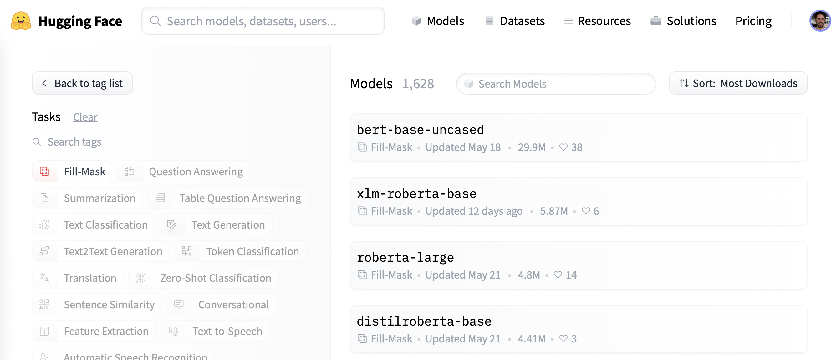
Although the BERT and RoBERTa family of models are the most downloaded, we’ll use a model called DistilBERT that can be trained much faster with little to no loss in downstream performance. This model was trained using a special technique called knowledge distillation, where a large “teacher model” like BERT is used to guide the training of a “student model” that has far fewer parameters. An explanation of the details of knowledge distillation would take us too far afield in this section, but if you’re interested you can read all about it in Natural Language Processing with Transformers (colloquially known as the Transformers textbook).
Let’s go ahead and download DistilBERT using the AutoModelForMaskedLM class:
from transformers import AutoModelForMaskedLM

model_checkpoint = "distilbert-base-uncased"
model = AutoModelForMaskedLM.from_pretrained(model_checkpoint)
We can see how many parameters this model has by calling the num_parameters() method:
distilbert_num_parameters = model.num_parameters() / 1_000_000
print(f"'>>> DistilBERT number of parameters: {round(distilbert_num_parameters)}M'")
print(f"'>>> BERT number of parameters: 110M'")'>>> DistilBERT number of parameters: 67M'
'>>> BERT number of parameters: 110M'With around 67 million parameters, DistilBERT is approximately two times smaller than the BERT base model, which roughly translates into a two-fold speedup in training — nice! Let’s now see what kinds of tokens this model predicts are the most likely completions of a small sample of text:
text = "This is a great [MASK]."As humans, we can imagine many possibilities for the [MASK] token, such as “day”, “ride”, or “painting”. For pretrained models, the predictions depend on the corpus the model was trained on, since it learns to pick up the statistical patterns present in the data. Like BERT, DistilBERT was pretrained on the English Wikipedia and BookCorpus datasets, so we expect the predictions for [MASK] to reflect these domains. To predict the mask we need DistilBERT’s tokenizer to produce the inputs for the model, so let’s download that from the Hub as well:
from transformers import AutoTokenizer

tokenizer = AutoTokenizer.from_pretrained(model_checkpoint)
With a tokenizer and a model, we can now pass our text example to the model, extract the logits, and print out the top 5 candidates:
import torch

inputs = tokenizer(text, return_tensors="pt")
token_logits = model(**inputs).logits
# Find the location of [MASK] and extract its logits
mask_token_index = torch.where(inputs["input_ids"] == tokenizer.mask_token_id)[1]
mask_token_logits = token_logits[0, mask_token_index, :]
# Pick the [MASK] candidates with the highest logits
top_5_tokens = torch.topk(mask_token_logits, 5, dim=1).indices[0].tolist()

for token in top_5_tokens:
print(f"'>>> {text.replace(tokenizer.mask_token, tokenizer.decode([token]))}'")'>>> This is a great deal.'
'>>> This is a great success.'
'>>> This is a great adventure.'
'>>> This is a great idea.'
'>>> This is a great feat.'We can see from the outputs that the model’s predictions refer to everyday terms, which is perhaps not surprising given the foundation of English Wikipedia. Let’s see how we can change this domain to something a bit more niche — highly polarized movie reviews!
The dataset
To showcase domain adaptation, we’ll use the famous Large Movie Review Dataset (or IMDb for short), which is a corpus of movie reviews that is often used to benchmark sentiment analysis models. By fine-tuning DistilBERT on this corpus, we expect the language model will adapt its vocabulary from the factual data of Wikipedia that it was pretrained on to the more subjective elements of movie reviews. We can get the data from the Hugging Face Hub with the load_dataset() function from 🤗 Datasets:
from datasets import load_dataset

imdb_dataset = load_dataset("imdb")
imdb_datasetDatasetDict({
train: Dataset({
features: ['text', 'label'],
num_rows: 25000
})
test: Dataset({
features: ['text', 'label'],
num_rows: 25000
})
unsupervised: Dataset({
features: ['text', 'label'],
num_rows: 50000
})
})We can see that the train and test splits each consist of 25,000 reviews, while there is an unlabeled split called unsupervised that contains 50,000 reviews. Let’s take a look at a few samples to get an idea of what kind of text we’re dealing with. As we’ve done in previous chapters of the course, we’ll chain the Dataset.shuffle() and Dataset.select() functions to create a random sample:
sample = imdb_dataset["train"].shuffle(seed=42).select(range(3))

for row in sample:
    print(f"\n'>>> Review: {row['text']}'")
    print(f"'>>> Label: {row['label']}'")
'>>> Review: This is your typical Priyadarshan movie--a bunch of loony characters out on some silly mission. His signature climax has the entire cast of the film coming together and fighting each other in some crazy moshpit over hidden money. Whether it is a winning lottery ticket in Malamaal Weekly, black money in Hera Pheri, "kodokoo" in Phir Hera Pheri, etc., etc., the director is becoming ridiculously predictable. Don\'t get me wrong; as clichéd and preposterous his movies may be, I usually end up enjoying the comedy. However, in most his previous movies there has actually been some good humor, (Hungama and Hera Pheri being noteworthy ones). Now, the hilarity of his films is fading as he is using the same formula over and over again.<br /><br />Songs are good. Tanushree Datta looks awesome. Rajpal Yadav is irritating, and Tusshar is not a whole lot better. Kunal Khemu is OK, and Sharman Joshi is the best.'
'>>> Label: 0'

'>>> Review: Okay, the story makes no sense, the characters lack any dimensionally, the best dialogue is ad-libs about the low quality of movie, the cinematography is dismal, and only editing saves a bit of the muddle, but Sam" Peckinpah directed the film. Somehow, his direction is not enough. For those who appreciate Peckinpah and his great work, this movie is a disappointment. Even a great cast cannot redeem the time the viewer wastes with this minimal effort.<br /><br />The proper response to the movie is the contempt that the director San Peckinpah, James Caan, Robert Duvall, Burt Young, Bo Hopkins, Arthur Hill, and even Gig Young bring to their work. Watch the great Peckinpah films. Skip this mess.'
'>>> Label: 0'

'>>> Review: I saw this movie at the theaters when I was about 6 or 7 years old. I loved it then, and have recently come to own a VHS version. <br /><br />My 4 and 6 year old children love this movie and have been asking again and again to watch it. <br /><br />I have enjoyed watching it again too. Though I have to admit it is not as good on a little TV.<br /><br />I do not have older children so I do not know what they would think of it. <br /><br />The songs are very cute. My daughter keeps singing them over and over.<br /><br />Hope this helps.'
'>>> Label: 1'
Yep, these are certainly movie reviews, and if you’re old enough you may even understand the comment in the last review about owning a VHS version 😜! Although we won’t need the labels for language modeling, we can already see that a 0 denotes a negative review, while a 1 corresponds to a positive one.
✏️ Try it out! Create a random sample of the unsupervised split and verify that the labels are neither 0 nor 1. While you’re at it, you could also check that the labels in the train and test splits are indeed 0 or 1 — this is a useful sanity check that every NLP practitioner should perform at the start of a new project!
Now that we’ve had a quick look at the data, let’s dive into preparing it for masked language modeling. As we’ll see, there are some additional steps that one needs to take compared to the sequence classification tasks we saw in Chapter 3. Let’s go!
Preprocessing the data
For both auto-regressive and masked language modeling, a common preprocessing step is to concatenate all the examples and then split the whole corpus into chunks of equal size. This is quite different from our usual approach, where we simply tokenize individual examples. Why concatenate everything together? The reason is that individual examples might get truncated if they’re too long, and that would result in losing information that might be useful for the language modeling task!
So to get started, we’ll first tokenize our corpus as usual, but without setting the truncation=True option in our tokenizer. We’ll also grab the word IDs if they are available ((which they will be if we’re using a fast tokenizer, as described in Chapter 6), as we will need them later on to do whole word masking. We’ll wrap this in a simple function, and while we’re at it we’ll remove the text and label columns since we don’t need them any longer:
def tokenize_function(examples):
    result = tokenizer(examples["text"])
    if tokenizer.is_fast:
        result["word_ids"] = [result.word_ids(i) for i in range(len(result["input_ids"]))]
    return result


# Use batched=True to activate fast multithreading!
tokenized_datasets = imdb_dataset.map(
    tokenize_function, batched=True, remove_columns=["text", "label"]
)
tokenized_datasetsDatasetDict({
train: Dataset({
features: ['attention_mask', 'input_ids', 'word_ids'],
num_rows: 25000
})
test: Dataset({
features: ['attention_mask', 'input_ids', 'word_ids'],
num_rows: 25000
})
unsupervised: Dataset({
features: ['attention_mask', 'input_ids', 'word_ids'],
num_rows: 50000
})
})Since DistilBERT is a BERT-like model, we can see that the encoded texts consist of the input_ids and attention_mask that we’ve seen in other chapters, as well as the word_ids we added.
Now that we’ve tokenized our movie reviews, the next step is to group them all together and split the result into chunks. But how big should these chunks be? This will ultimately be determined by the amount of GPU memory that you have available, but a good starting point is to see what the model’s maximum context size is. This can be inferred by inspecting the model_max_length attribute of the tokenizer:
tokenizer.model_max_length
512This value is derived from the tokenizer_config.json file associated with a checkpoint; in this case we can see that the context size is 512 tokens, just like with BERT.
✏️ Try it out! Some Transformer models, like BigBird and Longformer, have a much longer context length than BERT and other early Transformer models. Instantiate the tokenizer for one of these checkpoints and verify that the model_max_length agrees with what’s quoted on its model card.
So, in order to run our experiments on GPUs like those found on Google Colab, we’ll pick something a bit smaller that can fit in memory:
chunk_size = 128Note that using a small chunk size can be detrimental in real-world scenarios, so you should use a size that corresponds to the use case you will apply your model to.
Now comes the fun part. To show how the concatenation works, let’s take a few reviews from our tokenized training set and print out the number of tokens per review:
# Slicing produces a list of lists for each feature
tokenized_samples = tokenized_datasets["train"][:3]

for idx, sample in enumerate(tokenized_samples["input_ids"]):
print(f"'>>> Review {idx} length: {len(sample)}'")'>>> Review 0 length: 200'
'>>> Review 1 length: 559'
'>>> Review 2 length: 192'We can then concatenate all these examples with a simple dictionary comprehension, as follows:
concatenated_examples = {
    k: sum(tokenized_samples[k], []) for k in tokenized_samples.keys()
}
total_length = len(concatenated_examples["input_ids"])
print(f"'>>> Concatenated reviews length: {total_length}'")'>>> Concatenated reviews length: 951'Great, the total length checks out — so now let’s split the concatenated reviews into chunks of the size given by chunk_size. To do so, we iterate over the features in concatenated_examples and use a list comprehension to create slices of each feature. The result is a dictionary of chunks for each feature:
chunks = {
    k: [t[i : i + chunk_size] for i in range(0, total_length, chunk_size)]
    for k, t in concatenated_examples.items()
}

for chunk in chunks["input_ids"]:
print(f"'>>> Chunk length: {len(chunk)}'")'>>> Chunk length: 128'
'>>> Chunk length: 128'
'>>> Chunk length: 128'
'>>> Chunk length: 128'
'>>> Chunk length: 128'
'>>> Chunk length: 128'
'>>> Chunk length: 128'
'>>> Chunk length: 55'As you can see in this example, the last chunk will generally be smaller than the maximum chunk size. There are two main strategies for dealing with this:
- Drop the last chunk if it’s smaller than
chunk_size. - Pad the last chunk until its length equals
chunk_size.
We’ll take the first approach here, so let’s wrap all of the above logic in a single function that we can apply to our tokenized datasets:
def group_texts(examples):
    # Concatenate all texts
    concatenated_examples = {k: sum(examples[k], []) for k in examples.keys()}
    # Compute length of concatenated texts
    total_length = len(concatenated_examples[list(examples.keys())[0]])
    # We drop the last chunk if it's smaller than chunk_size
    total_length = (total_length // chunk_size) * chunk_size
    # Split by chunks of max_len
    result = {
        k: [t[i : i + chunk_size] for i in range(0, total_length, chunk_size)]
        for k, t in concatenated_examples.items()
    }
    # Create a new labels column
    result["labels"] = result["input_ids"].copy()
    return result
Note that in the last step of group_texts() we create a new labels column which is a copy of the input_ids one. As we’ll see shortly, that’s because in masked language modeling the objective is to predict randomly masked tokens in the input batch, and by creating a labels column we provide the ground truth for our language model to learn from.
Let’s now apply group_texts() to our tokenized datasets using our trusty Dataset.map() function:
lm_datasets = tokenized_datasets.map(group_texts, batched=True)
lm_datasetsDatasetDict({
train: Dataset({
features: ['attention_mask', 'input_ids', 'labels', 'word_ids'],
num_rows: 61289
})
test: Dataset({
features: ['attention_mask', 'input_ids', 'labels', 'word_ids'],
num_rows: 59905
})
unsupervised: Dataset({
features: ['attention_mask', 'input_ids', 'labels', 'word_ids'],
num_rows: 122963
})
})You can see that grouping and then chunking the texts has produced many more examples than our original 25,000 for the train and test splits. That’s because we now have examples involving contiguous tokens that span across multiple examples from the original corpus. You can see this explicitly by looking for the special [SEP] and [CLS] tokens in one of the chunks:
tokenizer.decode(lm_datasets["train"][1]["input_ids"])".... at.......... high. a classic line : inspector : i'm here to sack one of your teachers. student : welcome to bromwell high. i expect that many adults of my age think that bromwell high is far fetched. what a pity that it isn't! [SEP] [CLS] homelessness ( or houselessness as george carlin stated ) has been an issue for years but never a plan to help those on the street that were once considered human who did everything from going to school, work, or vote for the matter. most people think of the homeless"In this example you can see two overlapping movie reviews, one about a high school movie and the other about homelessness. Let’s also check out what the labels look like for masked language modeling:
tokenizer.decode(lm_datasets["train"][1]["labels"])".... at.......... high. a classic line : inspector : i'm here to sack one of your teachers. student : welcome to bromwell high. i expect that many adults of my age think that bromwell high is far fetched. what a pity that it isn't! [SEP] [CLS] homelessness ( or houselessness as george carlin stated ) has been an issue for years but never a plan to help those on the street that were once considered human who did everything from going to school, work, or vote for the matter. most people think of the homeless"As expected from our group_texts() function above, this looks identical to the decoded input_ids — but then how can our model possibly learn anything? We’re missing a key step: inserting [MASK] tokens at random positions in the inputs! Let’s see how we can do this on the fly during fine-tuning using a special data collator.
Fine-tuning DistilBERT with the Trainer API
Fine-tuning a masked language model is almost identical to fine-tuning a sequence classification model, like we did in Chapter 3. The only difference is that we need a special data collator that can randomly mask some of the tokens in each batch of texts. Fortunately, 🤗 Transformers comes prepared with a dedicated DataCollatorForLanguageModeling for just this task. We just have to pass it the tokenizer and an mlm_probability argument that specifies what fraction of the tokens to mask. We’ll pick 15%, which is the amount used for BERT and a common choice in the literature:
from transformers import DataCollatorForLanguageModeling

data_collator = DataCollatorForLanguageModeling(tokenizer=tokenizer, mlm_probability=0.15)
To see how the random masking works, let’s feed a few examples to the data collator. Since it expects a list of dicts, where each dict represents a single chunk of contiguous text, we first iterate over the dataset before feeding the batch to the collator. We remove the "word_ids" key for this data collator as it does not expect it:
samples = [lm_datasets["train"][i] for i in range(2)]
for sample in samples:
    _ = sample.pop("word_ids")

for chunk in data_collator(samples)["input_ids"]:
print(f"\n'>>> {tokenizer.decode(chunk)}'")'>>> [CLS] bromwell [MASK] is a cartoon comedy. it ran at the same [MASK] as some other [MASK] about school life, [MASK] as " teachers ". [MASK] [MASK] [MASK] in the teaching [MASK] lead [MASK] to believe that bromwell high\'[MASK] satire is much closer to reality than is " teachers ". the scramble [MASK] [MASK] financially, the [MASK]ful students whogn [MASK] right through [MASK] pathetic teachers\'pomp, the pettiness of the whole situation, distinction remind me of the schools i knew and their students. when i saw [MASK] episode in [MASK] a student repeatedly tried to burn down the school, [MASK] immediately recalled. [MASK]...'
'>>> .... at.. [MASK]... [MASK]... high. a classic line plucked inspector : i\'[MASK] here to [MASK] one of your [MASK]. student : welcome to bromwell [MASK]. i expect that many adults of my age think that [MASK]mwell [MASK] is [MASK] fetched. what a pity that it isn\'t! [SEP] [CLS] [MASK]ness ( or [MASK]lessness as george 宇in stated )公 been an issue for years but never [MASK] plan to help those on the street that were once considered human [MASK] did everything from going to school, [MASK], [MASK] vote for the matter. most people think [MASK] the homeless'Nice, it worked! We can see that the [MASK] token has been randomly inserted at various locations in our text. These will be the tokens which our model will have to predict during training — and the beauty of the data collator is that it will randomize the [MASK] insertion with every batch!
✏️ Try it out! Run the code snippet above several times to see the random masking happen in front of your very eyes! Also replace the tokenizer.decode() method with tokenizer.convert_ids_to_tokens() to see that sometimes a single token from a given word is masked, and not the others.
One side effect of random masking is that our evaluation metrics will not be deterministic when using the Trainer, since we use the same data collator for the training and test sets. We’ll see later, when we look at fine-tuning with 🤗 Accelerate, how we can use the flexibility of a custom evaluation loop to freeze the randomness.
When training models for masked language modeling, one technique that can be used is to mask whole words together, not just individual tokens. This approach is called whole word masking. If we want to use whole word masking, we will need to build a data collator ourselves. A data collator is just a function that takes a list of samples and converts them into a batch, so let’s do this now! We’ll use the word IDs computed earlier to make a map between word indices and the corresponding tokens, then randomly decide which words to mask and apply that mask on the inputs. Note that the labels are all -100 except for the ones corresponding to mask words.
import collections
import numpy as np

from transformers import default_data_collator

wwm_probability = 0.2


def whole_word_masking_data_collator(features):
    for feature in features:
        word_ids = feature.pop("word_ids")

        # Create a map between words and corresponding token indices
        mapping = collections.defaultdict(list)
        current_word_index = -1
        current_word = None
        for idx, word_id in enumerate(word_ids):
            if word_id is not None:
                if word_id != current_word:
                    current_word = word_id
                    current_word_index += 1
                mapping[current_word_index].append(idx)

        # Randomly mask words
        mask = np.random.binomial(1, wwm_probability, (len(mapping),))
        input_ids = feature["input_ids"]
        labels = feature["labels"]
        new_labels = [-100] * len(labels)
        for word_id in np.where(mask)[0]:
            word_id = word_id.item()
            for idx in mapping[word_id]:
                new_labels[idx] = labels[idx]
                input_ids[idx] = tokenizer.mask_token_id
        feature["labels"] = new_labels

    return default_data_collator(features)
Next, we can try it on the same samples as before:
samples = [lm_datasets["train"][i] for i in range(2)]
batch = whole_word_masking_data_collator(samples)

for chunk in batch["input_ids"]:
print(f"\n'>>> {tokenizer.decode(chunk)}'")'>>> [CLS] bromwell high is a cartoon comedy [MASK] it ran at the same time as some other programs about school life, such as " teachers ". my 35 years in the teaching profession lead me to believe that bromwell high\'s satire is much closer to reality than is " teachers ". the scramble to survive financially, the insightful students who can see right through their pathetic teachers\'pomp, the pettiness of the whole situation, all remind me of the schools i knew and their students. when i saw the episode in which a student repeatedly tried to burn down the school, i immediately recalled.....'
'>>> .... [MASK] [MASK] [MASK] [MASK]....... high. a classic line : inspector : i\'m here to sack one of your teachers. student : welcome to bromwell high. i expect that many adults of my age think that bromwell high is far fetched. what a pity that it isn\'t! [SEP] [CLS] homelessness ( or houselessness as george carlin stated ) has been an issue for years but never a plan to help those on the street that were once considered human who did everything from going to school, work, or vote for the matter. most people think of the homeless'✏️ Try it out! Run the code snippet above several times to see the random masking happen in front of your very eyes! Also replace the tokenizer.decode() method with tokenizer.convert_ids_to_tokens() to see that the tokens from a given word are always masked together.
Now that we have two data collators, the rest of the fine-tuning steps are standard. Training can take a while on Google Colab if you’re not lucky enough to score a mythical P100 GPU 😭, so we’ll first downsample the size of the training set to a few thousand examples. Don’t worry, we’ll still get a pretty decent language model! A quick way to downsample a dataset in 🤗 Datasets is via the Dataset.train_test_split() function that we saw in Chapter 5:
train_size = 10_000
test_size = int(0.1 * train_size)

downsampled_dataset = lm_datasets["train"].train_test_split(
    train_size=train_size, test_size=test_size, seed=42
)
downsampled_datasetDatasetDict({
train: Dataset({
features: ['attention_mask', 'input_ids', 'labels', 'word_ids'],
num_rows: 10000
})
test: Dataset({
features: ['attention_mask', 'input_ids', 'labels', 'word_ids'],
num_rows: 1000
})
})This has automatically created new train and test splits, with the training set size set to 10,000 examples and the validation set to 10% of that — feel free to increase this if you have a beefy GPU! The next thing we need to do is log in to the Hugging Face Hub. If you’re running this code in a notebook, you can do so with the following utility function:
from huggingface_hub import notebook_login

notebook_login()
which will display a widget where you can enter your credentials. Alternatively, you can run:
huggingface-cli loginin your favorite terminal and log in there.
Once we’re logged in, we can specify the arguments for the Trainer:
from transformers import TrainingArguments

batch_size = 64
# Show the training loss with every epoch
logging_steps = len(downsampled_dataset["train"]) // batch_size
model_name = model_checkpoint.split("/")[-1]

training_args = TrainingArguments(
    output_dir=f"{model_name}-finetuned-imdb",
    overwrite_output_dir=True,
    evaluation_strategy="epoch",
    learning_rate=2e-5,
    weight_decay=0.01,
    per_device_train_batch_size=batch_size,
    per_device_eval_batch_size=batch_size,
    push_to_hub=True,
    fp16=True,
    logging_steps=logging_steps,
)
Here we tweaked a few of the default options, including logging_steps to ensure we track the training loss with each epoch. We’ve also used fp16=True to enable mixed-precision training, which gives us another boost in speed. By default, the Trainer will remove any columns that are not part of the model’s forward() method. This means that if you’re using the whole word masking collator, you’ll also need to set remove_unused_columns=False to ensure we don’t lose the word_ids column during training.
Note that you can specify the name of the repository you want to push to with the hub_model_id argument (in particular, you will have to use this argument to push to an organization). For instance, when we pushed the model to the huggingface-course organization, we added hub_model_id="huggingface-course/distilbert-finetuned-imdb" to TrainingArguments. By default, the repository used will be in your namespace and named after the output directory you set, so in our case it will be "lewtun/distilbert-finetuned-imdb".
We now have all the ingredients to instantiate the Trainer. Here we just use the standard data_collator, but you can try the whole word masking collator and compare the results as an exercise:
from transformers import Trainer

trainer = Trainer(
    model=model,
    args=training_args,
    train_dataset=downsampled_dataset["train"],
    eval_dataset=downsampled_dataset["test"],
    data_collator=data_collator,
    tokenizer=tokenizer,
)
We’re now ready to run trainer.train() — but before doing so let’s briefly look at perplexity, which is a common metric to evaluate the performance of language models.
Perplexity for language models
Unlike other tasks like text classification or question answering where we’re given a labeled corpus to train on, with language modeling we don’t have any explicit labels. So how do we determine what makes a good language model? Like with the autocorrect feature in your phone, a good language model is one that assigns high probabilities to sentences that are grammatically correct, and low probabilities to nonsense sentences. To give you a better idea of what this looks like, you can find whole sets of “autocorrect fails” online, where the model in a person’s phone has produced some rather funny (and often inappropriate) completions!
Assuming our test set consists mostly of sentences that are grammatically correct, then one way to measure the quality of our language model is to calculate the probabilities it assigns to the next word in all the sentences of the test set. High probabilities indicates that the model is not “surprised” or “perplexed” by the unseen examples, and suggests it has learned the basic patterns of grammar in the language. There are various mathematical definitions of perplexity, but the one we’ll use defines it as the exponential of the cross-entropy loss. Thus, we can calculate the perplexity of our pretrained model by using the Trainer.evaluate() function to compute the cross-entropy loss on the test set and then taking the exponential of the result:
import math

eval_results = trainer.evaluate()
print(f">>> Perplexity: {math.exp(eval_results['eval_loss']):.2f}")>>> Perplexity: 21.75A lower perplexity score means a better language model, and we can see here that our starting model has a somewhat large value. Let’s see if we can lower it by fine-tuning! To do that, we first run the training loop:
trainer.train()
and then compute the resulting perplexity on the test set as before:
eval_results = trainer.evaluate()
print(f">>> Perplexity: {math.exp(eval_results['eval_loss']):.2f}")>>> Perplexity: 11.32Nice — this is quite a reduction in perplexity, which tells us the model has learned something about the domain of movie reviews!
Once training is finished, we can push the model card with the training information to the Hub (the checkpoints are saved during training itself):
trainer.push_to_hub()
✏️ Your turn! Run the training above after changing the data collator to the whole word masking collator. Do you get better results?
In our use case we didn’t need to do anything special with the training loop, but in some cases you might need to implement some custom logic. For these applications, you can use 🤗 Accelerate — let’s take a look!
Fine-tuning DistilBERT with 🤗 Accelerate
As we saw with the Trainer, fine-tuning a masked language model is very similar to the text classification example from Chapter 3. In fact, the only subtlety is the use of a special data collator, and we’ve already covered that earlier in this section!
However, we saw that DataCollatorForLanguageModeling also applies random masking with each evaluation, so we’ll see some fluctuations in our perplexity scores with each training run. One way to eliminate this source of randomness is to apply the masking once on the whole test set, and then use the default data collator in 🤗 Transformers to collect the batches during evaluation. To see how this works, let’s implement a simple function that applies the masking on a batch, similar to our first encounter with DataCollatorForLanguageModeling:
def insert_random_mask(batch):
    features = [dict(zip(batch, t)) for t in zip(*batch.values())]
    masked_inputs = data_collator(features)
    # Create a new "masked" column for each column in the dataset
    return {"masked_" + k: v.numpy() for k, v in masked_inputs.items()}
Next, we’ll apply this function to our test set and drop the unmasked columns so we can replace them with the masked ones. You can use whole word masking by replacing the data_collator above with the appropriate one, in which case you should remove the first line here:
downsampled_dataset = downsampled_dataset.remove_columns(["word_ids"])
eval_dataset = downsampled_dataset["test"].map(
    insert_random_mask,
    batched=True,
    remove_columns=downsampled_dataset["test"].column_names,
)
eval_dataset = eval_dataset.rename_columns(
    {
        "masked_input_ids": "input_ids",
        "masked_attention_mask": "attention_mask",
        "masked_labels": "labels",
    }
)
We can then set up the dataloaders as usual, but we’ll use the default_data_collator from 🤗 Transformers for the evaluation set:
from torch.utils.data import DataLoader
from transformers import default_data_collator

batch_size = 64
train_dataloader = DataLoader(
    downsampled_dataset["train"],
    shuffle=True,
    batch_size=batch_size,
    collate_fn=data_collator,
)
eval_dataloader = DataLoader(
    eval_dataset, batch_size=batch_size, collate_fn=default_data_collator
)
Form here, we follow the standard steps with 🤗 Accelerate. The first order of business is to load a fresh version of the pretrained model:
model = AutoModelForMaskedLM.from_pretrained(model_checkpoint)Then we need to specify the optimizer; we’ll use the standard AdamW:
from torch.optim import AdamW

optimizer = AdamW(model.parameters(), lr=5e-5)
With these objects, we can now prepare everything for training with the Accelerator object:
from accelerate import Accelerator

accelerator = Accelerator()
model, optimizer, train_dataloader, eval_dataloader = accelerator.prepare(
    model, optimizer, train_dataloader, eval_dataloader
)
Now that our model, optimizer, and dataloaders are configured, we can specify the learning rate scheduler as follows:
from transformers import get_scheduler

num_train_epochs = 3
num_update_steps_per_epoch = len(train_dataloader)
num_training_steps = num_train_epochs * num_update_steps_per_epoch

lr_scheduler = get_scheduler(
    "linear",
    optimizer=optimizer,
    num_warmup_steps=0,
    num_training_steps=num_training_steps,
)
There is just one last thing to do before training: create a model repository on the Hugging Face Hub! We can use the 🤗 Hub library to first generate the full name of our repo:
from huggingface_hub import get_full_repo_name

model_name = "distilbert-base-uncased-finetuned-imdb-accelerate"
repo_name = get_full_repo_name(model_name)
repo_name'lewtun/distilbert-base-uncased-finetuned-imdb-accelerate'then create and clone the repository using the Repository class from 🤗 Hub:
from huggingface_hub import Repository

output_dir = model_name
repo = Repository(output_dir, clone_from=repo_name)
With that done, it’s just a simple matter of writing out the full training and evaluation loop:
from tqdm.auto import tqdm
import torch
import math

progress_bar = tqdm(range(num_training_steps))

for epoch in range(num_train_epochs):
    # Training
    model.train()
    for batch in train_dataloader:
        outputs = model(**batch)
        loss = outputs.loss
        accelerator.backward(loss)

        optimizer.step()
        lr_scheduler.step()
        optimizer.zero_grad()
        progress_bar.update(1)

    # Evaluation
    model.eval()
    losses = []
    for step, batch in enumerate(eval_dataloader):
        with torch.no_grad():
            outputs = model(**batch)

        loss = outputs.loss
        losses.append(accelerator.gather(loss.repeat(batch_size)))

    losses = torch.cat(losses)
    losses = losses[: len(eval_dataset)]
    try:
        perplexity = math.exp(torch.mean(losses))
    except OverflowError:
        perplexity = float("inf")

    print(f">>> Epoch {epoch}: Perplexity: {perplexity}")

    # Save and upload
    accelerator.wait_for_everyone()
    unwrapped_model = accelerator.unwrap_model(model)
    unwrapped_model.save_pretrained(output_dir, save_function=accelerator.save)
    if accelerator.is_main_process:
        tokenizer.save_pretrained(output_dir)
        repo.push_to_hub(
            commit_message=f"Training in progress epoch {epoch}", blocking=False
)>>> Epoch 0: Perplexity: 11.397545307900472
>>> Epoch 1: Perplexity: 10.904909330983092
>>> Epoch 2: Perplexity: 10.729503505340409Cool, we’ve been able to evaluate perplexity with each epoch and ensure that multiple training runs are reproducible!
Using our fine-tuned model
You can interact with your fine-tuned model either by using its widget on the Hub or locally with the pipeline from 🤗 Transformers. Let’s use the latter to download our model using the fill-mask pipeline:
from transformers import pipeline

mask_filler = pipeline(
    "fill-mask", model="huggingface-course/distilbert-base-uncased-finetuned-imdb"
)
We can then feed the pipeline our sample text of “This is a great [MASK]” and see what the top 5 predictions are:
preds = mask_filler(text)

for pred in preds:
print(f">>> {pred['sequence']}")'>>> this is a great movie.'
'>>> this is a great film.'
'>>> this is a great story.'
'>>> this is a great movies.'
'>>> this is a great character.'Neat — our model has clearly adapted its weights to predict words that are more strongly associated with movies!
This wraps up our first experiment with training a language model. In section 6 you’ll learn how to train an auto-regressive model like GPT-2 from scratch; head over there if you’d like to see how you can pretrain your very own Transformer model!
✏️ Try it out! To quantify the benefits of domain adaptation, fine-tune a classifier on the IMDb labels for both the pretrained and fine-tuned DistilBERT checkpoints. If you need a refresher on text classification, check out Chapter 3.