Transformers documentation
Efficient Training on Multiple GPUs
Efficient Training on Multiple GPUs
If training a model on a single GPU is too slow or if the model’s weights do not fit in a single GPU’s memory, transitioning to a multi-GPU setup may be a viable option. Prior to making this transition, thoroughly explore all the strategies covered in the Methods and tools for efficient training on a single GPU as they are universally applicable to model training on any number of GPUs. Once you have employed those strategies and found them insufficient for your case on a single GPU, consider moving to multiple GPUs.
Transitioning from a single GPU to multiple GPUs requires the introduction of some form of parallelism, as the workload must be distributed across the resources. Multiple techniques can be employed to achieve parallelism, such as data parallelism, tensor parallelism, and pipeline parallelism. It’s important to note that there isn’t a one-size-fits-all solution, and the optimal settings depend on the specific hardware configuration you are using.
This guide offers an in-depth overview of individual types of parallelism, as well as guidance on ways to combine
techniques and choosing an appropriate approach. For step-by-step tutorials on distributed training, please refer to
the 🤗 Accelerate documentation.
While the main concepts discussed in this guide are likely applicable across frameworks, here we focus on PyTorch-based implementations.
Before diving deeper into the specifics of each technique, let’s go over the rough decision process when training large models on a large infrastructure.
Scalability strategy
Begin by estimating how much vRAM is required to train your model. For models hosted on the 🤗 Hub, use our Model Memory Calculator, which gives you accurate calculations within a few percent margin.
Parallelization strategy for a single Node / multi-GPU setup
When training a model on a single node with multiple GPUs, your choice of parallelization strategy can significantly impact performance. Here’s a breakdown of your options:
Case 1: Your model fits onto a single GPU
If your model can comfortably fit onto a single GPU, you have two primary options:
- DDP - Distributed DataParallel
- ZeRO - depending on the situation and configuration used, this method may or may not be faster, however, it’s worth experimenting with it.
Case 2: Your model doesn’t fit onto a single GPU:
If your model is too large for a single GPU, you have several alternatives to consider:
- PipelineParallel (PP)
- ZeRO
- TensorParallel (TP)
With very fast inter-node connectivity (e.g., NVLINK or NVSwitch) all three strategies (PP, ZeRO, TP) should result in similar performance. However, without these, PP will be faster than TP or ZeRO. The degree of TP may also make a difference. It’s best to experiment with your specific setup to determine the most suitable strategy.
TP is almost always used within a single node. That is TP size <= GPUs per node.
Case 3: Largest layer of your model does not fit onto a single GPU
- If you are not using ZeRO, you have to use TensorParallel (TP), because PipelineParallel (PP) alone won’t be sufficient to accommodate the large layer.
- If you are using ZeRO, additionally adopt techniques from the Methods and tools for efficient training on a single GPU.
Parallelization strategy for a multi-Node / multi-GPU setup
When you have fast inter-node connectivity (e.g., NVLINK or NVSwitch) consider using one of these options:
- ZeRO - as it requires close to no modifications to the model
- A combination of PipelineParallel(PP) with TensorParallel(TP) and DataParallel(DP) - this approach will result in fewer communications, but requires significant changes to the model
When you have slow inter-node connectivity and still low on GPU memory:
- Employ a combination of DataParallel(DP) with PipelineParallel(PP), TensorParallel(TP), and ZeRO.
In the following sections of this guide we dig deeper into how these different parallelism methods work.
Data Parallelism
Even with only 2 GPUs, you can readily leverage the accelerated training capabilities offered by PyTorch’s built-in features,
such as DataParallel (DP) and DistributedDataParallel (DDP). Note that
PyTorch documentation recommends to prefer
DistributedDataParallel (DDP) over DataParallel (DP) for multi-GPU training as it works for all models.
Let’s take a look at how these two methods work and what makes them different.
DataParallel vs DistributedDataParallel
To understand the key differences in inter-GPU communication overhead between the two methods, let’s review the processes per batch:
DDP:
- At the start time the main process replicates the model once from GPU 0 to the rest of GPUs
- Then for each batch:
- Each GPU directly consumes its mini-batch of data.
- During
backward, once the local gradients are ready, they are averaged across all processes.
DP:
For each batch:
- GPU 0 reads the batch of data and then sends a mini-batch to each GPU.
- The up-to-date model is replicated from GPU 0 to each GPU.
forwardis executed, and output from each GPU is sent to GPU 0 to compute the loss.- The loss is distributed from GPU 0 to all GPUs, and
backwardis run. - Gradients from each GPU are sent to GPU 0 and averaged.
Key differences include:
- DDP performs only a single communication per batch - sending gradients, while DP performs five different data exchanges per batch.
DDP copies data using torch.distributed, while DP copies data within
the process via Python threads (which introduces limitations associated with GIL). As a result,
DistributedDataParallel(DDP) is generally faster thanDataParallel(DP) unless you have slow GPU card inter-connectivity. - Under DP, GPU 0 performs significantly more work than other GPUs, resulting in GPU under-utilization.
- DDP supports distributed training across multiple machines, whereas DP does not.
This is not an exhaustive list of differences between DP and DDP, however, other nuances are out of scope of this guide. You can get a deeper understanding of these methods by reading this article.
Let’s illustrate the differences between DP and DDP with an experiment. We’ll benchmark the differences between DP and DDP with an added context of NVLink presence:
- Hardware: 2x TITAN RTX 24GB each + NVlink with 2 NVLinks (
NV2innvidia-smi topo -m). - Software:
pytorch-1.8-to-be+cuda-11.0/transformers==4.3.0.dev0.
To disable the NVLink feature on one of the benchmarks, we use NCCL_P2P_DISABLE=1.
Here is the benchmarking code and outputs:
DP
rm -r /tmp/test-clm; CUDA_VISIBLE_DEVICES=0,1 \
python examples/pytorch/language-modeling/run_clm.py \
--model_name_or_path gpt2 --dataset_name wikitext --dataset_config_name wikitext-2-raw-v1 \
--do_train --output_dir /tmp/test-clm --per_device_train_batch_size 4 --max_steps 200

{'train_runtime': 110.5948, 'train_samples_per_second': 1.808, 'epoch': 0.69}
DDP w/ NVlink
rm -r /tmp/test-clm; CUDA_VISIBLE_DEVICES=0,1 \
torchrun --nproc_per_node 2 examples/pytorch/language-modeling/run_clm.py \
--model_name_or_path gpt2 --dataset_name wikitext --dataset_config_name wikitext-2-raw-v1 \
--do_train --output_dir /tmp/test-clm --per_device_train_batch_size 4 --max_steps 200

{'train_runtime': 101.9003, 'train_samples_per_second': 1.963, 'epoch': 0.69}
DDP w/o NVlink
rm -r /tmp/test-clm; NCCL_P2P_DISABLE=1 CUDA_VISIBLE_DEVICES=0,1 \
torchrun --nproc_per_node 2 examples/pytorch/language-modeling/run_clm.py \
--model_name_or_path gpt2 --dataset_name wikitext --dataset_config_name wikitext-2-raw-v1 \
--do_train --output_dir /tmp/test-clm --per_device_train_batch_size 4 --max_steps 200

{'train_runtime': 131.4367, 'train_samples_per_second': 1.522, 'epoch': 0.69}
Here are the same benchmarking results gathered in a table for convenience:
| Type | NVlink | Time |
|---|---|---|
| 2:DP | Y | 110s |
| 2:DDP | Y | 101s |
| 2:DDP | N | 131s |
As you can see, in this case DP is ~10% slower than DDP with NVlink, but ~15% faster than DDP without NVlink. The real difference will depend on how much data each GPU needs to sync with the others - the more there is to sync, the more a slow link will impede the overall runtime.
ZeRO Data Parallelism
ZeRO-powered data parallelism (ZeRO-DP) is illustrated in the following diagram from this blog post.
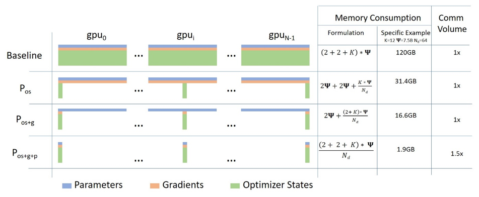
While it may appear complex, it is a very similar concept to DataParallel (DP). The difference is that instead of
replicating the full model parameters, gradients and optimizer states, each GPU stores only a slice of it. Then, at
run-time when the full layer parameters are needed just for the given layer, all GPUs synchronize to give each other
parts that they miss.
To illustrate this idea, consider a simple model with 3 layers (La, Lb, and Lc), where each layer has 3 parameters. Layer La, for example, has weights a0, a1 and a2:
La | Lb | Lc
---|----|---
a0 | b0 | c0
a1 | b1 | c1
a2 | b2 | c2
If we have 3 GPUs, ZeRO-DP splits the model onto 3 GPUs like so:
GPU0:
La | Lb | Lc
---|----|---
a0 | b0 | c0

GPU1:
La | Lb | Lc
---|----|---
a1 | b1 | c1

GPU2:
La | Lb | Lc
---|----|---
a2 | b2 | c2
In a way, this is the same horizontal slicing as tensor parallelism, as opposed to Vertical slicing, where one puts whole layer-groups on different GPUs. Now let’s see how this works:
Each of these GPUs will get the usual mini-batch as it works in DP:
x0 => GPU0
x1 => GPU1
x2 => GPU2
The inputs are passed without modifications as if they would be processed by the original model.
First, the inputs get to the layer La. What happens at this point?
On GPU0: the x0 mini-batch requires the a0, a1, a2 parameters to do its forward path through the layer, but the GPU0 has only a0. It will get a1 from GPU1 and a2 from GPU2, bringing all the pieces of the model together.
In parallel, GPU1 gets another mini-batch - x1. GPU1 has the a1 parameter, but needs a0 and a2, so it gets those from GPU0 and GPU2. Same happens to GPU2 that gets the mini-batch x2. It gets a0 and a1 from GPU0 and GPU1.
This way each of the 3 GPUs gets the full tensors reconstructed and makes a forward pass with its own mini-batch. As soon as the calculation is done, the data that is no longer needed gets dropped - it’s only used during the calculation. The reconstruction is done efficiently via a pre-fetch.
Then the whole process is repeated for layer Lb, then Lc forward-wise, and then backward Lc -> Lb -> La.
This mechanism is similar to an efficient group backpacking strategy: person A carries the tent, person B carries the stove, and person C carries the axe. Each night they all share what they have with others and get from others what they don’t have, and in the morning they pack up their allocated type of gear and continue on their way. This is what ZeRO DP/Sharded DDP is. Compare this strategy to the simple one where each person has to carry their own tent, stove and axe (similar to DataParallel (DP and DDP) in PyTorch), which would be far more inefficient.
While reading the literature on this topic you may encounter the following synonyms: Sharded, Partitioned. If you pay close attention the way ZeRO partitions the model’s weights - it looks very similar to tensor parallelism which will be discussed later. This is because it partitions/shards each layer’s weights, unlike vertical model parallelism which is discussed next.
Implementations:
- DeepSpeed ZeRO-DP stages 1+2+3
Accelerateintegrationtransformersintegration
From Naive Model Parallelism to Pipeline Parallelism
To explain Pipeline parallelism, we’ll first look into Naive Model Parallelism (MP), also known as Vertical MP. This approach
involves distributing groups of model layers across multiple GPUs by assigning specific layers to specific GPUs with .to().
As data flows through these layers, it is moved to the same GPU as the layer, while the other layers remain untouched.
We refer to this Model parallelism as “Vertical” because of how models are typically visualized. For example, the following diagram shows an 8-layer model split vertically into two slices, placing layers 0-3 onto GPU0 and 4-7 to GPU1:
===================  ===================
|  0 | 1 | 2 | 3  |  |  4 | 5 | 6 | 7  |
===================  ===================
        GPU0                 GPU1
In this example, when data moves from layer 0 to 3, it’s no different from regular forward pass. However, passing data from layer 3 to 4 requires moving it from GPU0 to GPU1, introducing a communication overhead. If the participating GPUs are on the same compute node (e.g. same physical machine) this copying is fast, but if the GPUs are distributed across different compute nodes (e.g. multiple machines), the communication overhead could be substantially greater.
Following that, layers 4 to 7 work as they would in the original model. Upon completion of the 7th layer, there is often a need to send the data back to layer 0 where the labels are (or alternatively send the labels to the last layer). Now the loss can be computed and the optimizer can do its work.
Naive Model Parallelism comes several shortcomings:
- All but one GPU are idle at any given moment: if 4 GPUs are used, it’s nearly identical to quadrupling the amount of memory of a single GPU, and ignoring the rest of the hardware.
- Overhead in data transfer between devices: E.g. 4x 6GB cards will be able to accommodate the same size as 1x 24GB card using naive MP, but a single 24GB card will complete the training faster, because it doesn’t have the data copying overhead. But, say, if you have 40GB cards and need to fit a 45GB model you can with 4x 40GB cards (but barely because of the gradient and optimizer states)
- Copying shared embeddings: Shared embeddings may need to get copied back and forth between GPUs.
Now that you are familiar with how the naive approach to model parallelism works and its shortcomings, let’s look at Pipeline Parallelism (PP). PP is almost identical to a naive MP, but it solves the GPU idling problem by chunking the incoming batch into micro-batches and artificially creating a pipeline, which allows different GPUs to concurrently participate in the computation process.
The following illustration from the GPipe paper shows the naive MP on the top, and PP on the bottom:
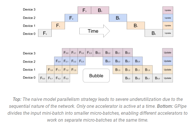
At the bottom of the diagram, you can observe that the Pipeline Parallelism (PP) approach minimizes the number of idle GPU zones, referred to as ‘bubbles’. Both parts of the diagram show a parallelism level of degree 4, meaning that 4 GPUs are involved in the pipeline. You can see that there’s a forward path of 4 pipe stages (F0, F1, F2 and F3) followed by a backward path in reverse order (B3, B2, B1, and B0).
PP introduces a new hyperparameter to tune - chunks, which determines how many data chunks are sent in a sequence
through the same pipe stage. For example, in the bottom diagram you can see chunks=4. GPU0 performs the same
forward path on chunk 0, 1, 2 and 3 (F0,0, F0,1, F0,2, F0,3) and then it waits for other GPUs to do complete their work.
Only when the other GPUs begin to complete their work, GPU0 starts to work again doing the backward path for chunks
3, 2, 1 and 0 (B0,3, B0,2, B0,1, B0,0).
Note that this is the same concept as gradient accumulation steps. PyTorch uses chunks, while DeepSpeed refers
to the same hyperparameter as gradient accumulation steps.
Because of the chunks, PP introduces the notion of micro-batches (MBS). DP splits the global data batch size into
mini-batches, so if you have a DP degree of 4, a global batch size of 1024 gets split up into 4 mini-batches of
256 each (1024/4). And if the number of chunks (or GAS) is 32 we end up with a micro-batch size of 8 (256/32). Each
Pipeline stage works with a single micro-batch at a time. To calculate the global batch size of the DP + PP setup,
use the formula: mbs * chunks * dp_degree (8 * 32 * 4 = 1024).
With chunks=1 you end up with the naive MP, which is inefficient. With a large chunks value you end up with
tiny micro-batch sizes which is also inefficient. For this reason, we encourage to experiment with the chunks value to
find the one that leads to the most efficient GPUs utilization.
You may notice a bubble of “dead” time on the diagram that can’t be parallelized because the last forward stage
has to wait for backward to complete the pipeline. The purpose of finding the best value for chunks is to enable a high
concurrent GPU utilization across all participating GPUs which translates to minimizing the size of the bubble.
Pipeline API solutions have been implemented in:
- PyTorch
- DeepSpeed
- Megatron-LM
These come with some shortcomings:
- They have to modify the model quite heavily, because Pipeline requires one to rewrite the normal flow of modules into a
nn.Sequentialsequence of the same, which may require changes to the design of the model. - Currently the Pipeline API is very restricted. If you had a bunch of Python variables being passed in the very first stage of the Pipeline, you will have to find a way around it. Currently, the pipeline interface requires either a single Tensor or a tuple of Tensors as the only input and output. These tensors must have a batch size as the very first dimension, since pipeline is going to chunk the mini batch into micro-batches. Possible improvements are being discussed here https://github.com/pytorch/pytorch/pull/50693
- Conditional control flow at the level of pipe stages is not possible - e.g., Encoder-Decoder models like T5 require special workarounds to handle a conditional encoder stage.
- They have to arrange each layer so that the output of one layer becomes an input to the other layer.
More recent solutions include:
- Varuna
- Sagemaker
We have not experimented with Varuna and SageMaker but their papers report that they have overcome the list of problems mentioned above and that they require smaller changes to the user’s model.
Implementations:
- PyTorch (initial support in pytorch-1.8, and progressively getting improved in 1.9 and more so in 1.10). Some examples
- DeepSpeed
- Megatron-LM has an internal implementation - no API.
- Varuna
- SageMaker - this is a proprietary solution that can only be used on AWS.
- OSLO - this is implemented based on the Hugging Face Transformers.
🤗 Transformers status: as of this writing none of the models supports full-PP. GPT2 and T5 models have naive MP support.
The main obstacle is being unable to convert the models to nn.Sequential and have all the inputs to be Tensors. This
is because currently the models include many features that make the conversion very complicated, and will need to be removed to accomplish that.
DeepSpeed and Megatron-LM integrations are available in 🤗 Accelerate
Other approaches:
DeepSpeed, Varuna and SageMaker use the concept of an Interleaved Pipeline

Here the bubble (idle time) is further minimized by prioritizing backward passes. Varuna further attempts to improve the schedule by using simulations to discover the most efficient scheduling.
OSLO has pipeline parallelism implementation based on the Transformers without nn.Sequential conversion.
Tensor Parallelism
In Tensor Parallelism, each GPU processes a slice of a tensor and only aggregates the full tensor for operations requiring it. To describe this method, this section of the guide relies on the concepts and diagrams from the Megatron-LM paper: Efficient Large-Scale Language Model Training on GPU Clusters.
The main building block of any transformer is a fully connected nn.Linear followed by a nonlinear activation GeLU.
The dot dot-product part of it, following the Megatron’s paper notation, can be written as Y = GeLU(XA), where X is
an input vector, Y is the output vector, and A is the weight matrix.
If we look at the computation in matrix form, you can see how the matrix multiplication can be split between multiple GPUs:
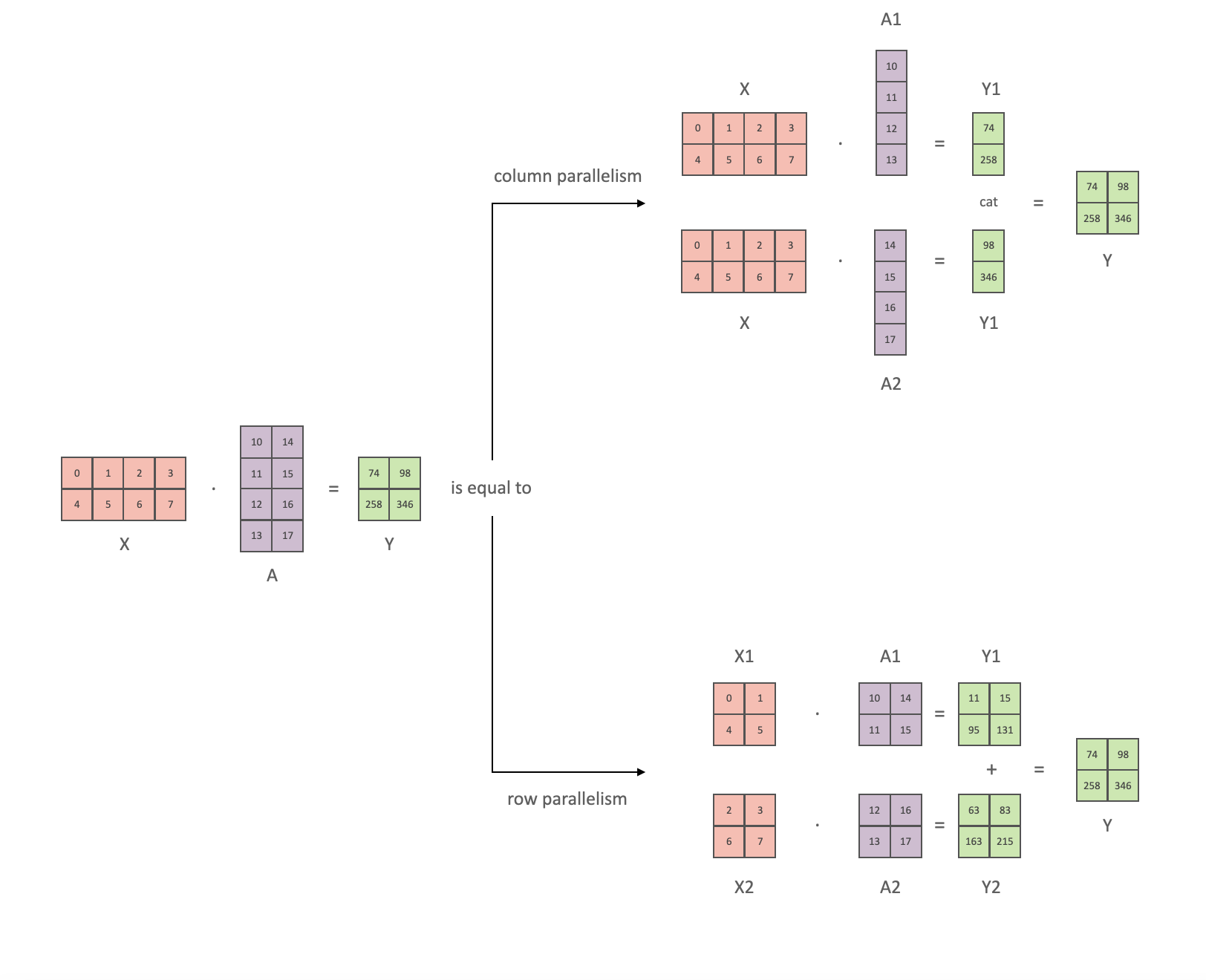
If we split the weight matrix A column-wise across N GPUs and perform matrix multiplications XA_1 through XA_n in parallel,
then we will end up with N output vectors Y_1, Y_2, ..., Y_n which can be fed into GeLU independently:

Using this principle, we can update a multi-layer perceptron of arbitrary depth, without the need for any synchronization between GPUs until the very end, where we need to reconstruct the output vector from shards. The Megatron-LM paper authors provide a helpful illustration for that:
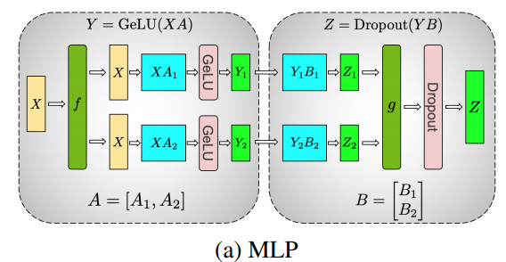
Parallelizing the multi-headed attention layers is even simpler, since they are already inherently parallel, due to having multiple independent heads!
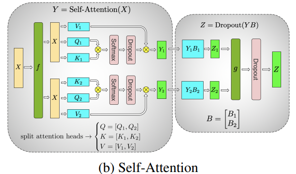
Special considerations: TP requires very fast network, and therefore it’s not advisable to do TP across more than one node. Practically, if a node has 4 GPUs, the highest TP degree is therefore 4. If you need a TP degree of 8, you need to use nodes that have at least 8 GPUs.
This section is based on the original much more detailed TP overview. by @anton-l.
Alternative names:
- DeepSpeed calls it tensor slicing
Implementations:
- Megatron-LM has an internal implementation, as it’s very model-specific
- parallelformers (only inference at the moment)
- SageMaker - this is a proprietary solution that can only be used on AWS.
- OSLO has the tensor parallelism implementation based on the Transformers.
SageMaker combines TP with DP for a more efficient processing.
🤗 Transformers status:
- core: not yet implemented in the core
- but if you want inference parallelformers provides this support for most of our models. So until this is implemented in the core you can use theirs. And hopefully training mode will be supported too.
- Deepspeed-Inference also supports our BERT, GPT-2, and GPT-Neo models in their super-fast CUDA-kernel-based inference mode, see more here
🤗 Accelerate integrates with TP from Megatron-LM.
Data Parallelism + Pipeline Parallelism
The following diagram from the DeepSpeed pipeline tutorial demonstrates how one can combine DP with PP.

Here it’s important to see how DP rank 0 doesn’t see GPU2 and DP rank 1 doesn’t see GPU3. To DP there is just GPUs 0 and 1 where it feeds data as if there were just 2 GPUs. GPU0 “secretly” offloads some of its load to GPU2 using PP. And GPU1 does the same by enlisting GPU3 to its aid.
Since each dimension requires at least 2 GPUs, here you’d need at least 4 GPUs.
Implementations:
🤗 Transformers status: not yet implemented
Data Parallelism + Pipeline Parallelism + Tensor Parallelism
To get an even more efficient training a 3D parallelism is used where PP is combined with TP and DP. This can be seen in the following diagram.
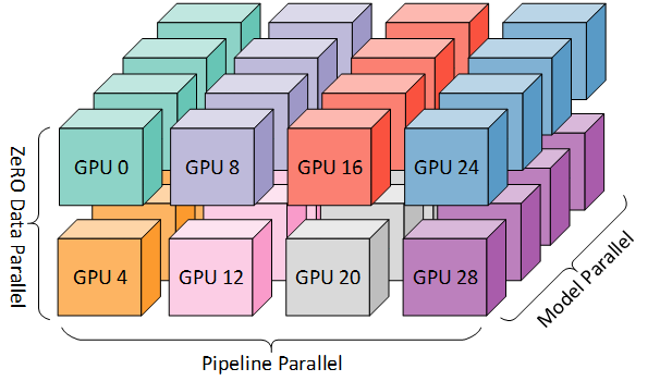
This diagram is from a blog post 3D parallelism: Scaling to trillion-parameter models, which is a good read as well.
Since each dimension requires at least 2 GPUs, here you’d need at least 8 GPUs.
Implementations:
- DeepSpeed - DeepSpeed also includes an even more efficient DP, which they call ZeRO-DP.
- Megatron-LM
- Varuna
- SageMaker
- OSLO
🤗 Transformers status: not yet implemented, since we have no PP and TP.
ZeRO Data Parallelism + Pipeline Parallelism + Tensor Parallelism
One of the main features of DeepSpeed is ZeRO, which is a super-scalable extension of DP. It has already been discussed in ZeRO Data Parallelism. Normally it’s a standalone feature that doesn’t require PP or TP. But it can be combined with PP and TP.
When ZeRO-DP is combined with PP (and optionally TP) it typically enables only ZeRO stage 1 (optimizer sharding).
While it’s theoretically possible to use ZeRO stage 2 (gradient sharding) with Pipeline Parallelism, it will have negative performance impacts. There would need to be an additional reduce-scatter collective for every micro-batch to aggregate the gradients before sharding, which adds a potentially significant communication overhead. By nature of Pipeline Parallelism, small micro-batches are used and instead the focus is on trying to balance arithmetic intensity (micro-batch size) with minimizing the Pipeline bubble (number of micro-batches). Therefore those communication costs are going to impact the performance.
In addition, there are already fewer layers than normal due to PP and so the memory savings won’t be huge. PP already
reduces gradient size by 1/PP, and so gradient sharding savings on top of that are less significant than pure DP.
ZeRO stage 3 is not a good choice either for the same reason - more inter-node communications required.
And since we have ZeRO, the other benefit is ZeRO-Offload. Since this is stage 1 optimizer states can be offloaded to CPU.
Implementations:
- Megatron-DeepSpeed and Megatron-Deepspeed from BigScience, which is the fork of the former repo.
- OSLO
Important papers:
🤗 Transformers status: not yet implemented, since we have no PP and TP.
FlexFlow
FlexFlow also solves the parallelization problem in a slightly different approach.
It performs a sort of 4D Parallelism over Sample-Operator-Attribute-Parameter.
- Sample = Data Parallelism (sample-wise parallel)
- Operator = Parallelize a single operation into several sub-operations
- Attribute = Data Parallelism (length-wise parallel)
- Parameter = Model Parallelism (regardless of dimension - horizontal or vertical)
Examples:
- Sample
Let’s take 10 batches of sequence length 512. If we parallelize them by sample dimension into 2 devices, we get 10 x 512 which becomes be 5 x 2 x 512.
- Operator
If we perform layer normalization, we compute std first and mean second, and then we can normalize data. Operator parallelism allows computing std and mean in parallel. So if we parallelize them by operator dimension into 2 devices (cuda:0, cuda:1), first we copy input data into both devices, and cuda:0 computes std, cuda:1 computes mean at the same time.
- Attribute
We have 10 batches of 512 length. If we parallelize them by attribute dimension into 2 devices, 10 x 512 will be 10 x 2 x 256.
- Parameter
It is similar with tensor model parallelism or naive layer-wise model parallelism.
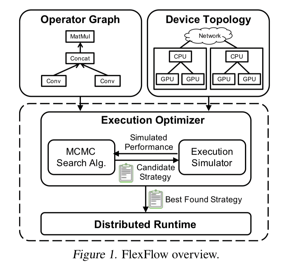
The significance of this framework is that it takes resources like (1) GPU/TPU/CPU vs. (2) RAM/DRAM vs. (3) fast-intra-connect/slow-inter-connect and it automatically optimizes all these algorithmically deciding which parallelisation to use where.
One very important aspect is that FlexFlow is designed for optimizing DNN parallelizations for models with static and fixed workloads, since models with dynamic behavior may prefer different parallelization strategies across iterations.
So the promise is very attractive - it runs a 30min simulation on the cluster of choice and it comes up with the best strategy to utilise this specific environment. If you add/remove/replace any parts it’ll run and re-optimize the plan for that. And then you can train. A different setup will have its own custom optimization.
🤗 Transformers status: Transformers models are FX-trace-able via transformers.utils.fx, which is a prerequisite for FlexFlow, however, changes are required on the FlexFlow side to make it work with Transformers models.
GPU selection
When training on multiple GPUs, you can specify the number of GPUs to use and in what order. This can be useful for instance when you have GPUs with different computing power and want to use the faster GPU first. The selection process works for both DistributedDataParallel and DataParallel to use only a subset of the available GPUs, and you don’t need Accelerate or the DeepSpeed integration.
Number of GPUs
For example, if you have 4 GPUs and you only want to use the first 2:
Use the --nproc_per_node to select how many GPUs to use.
torchrun --nproc_per_node=2 trainer-program.py ...
Order of GPUs
Now, to select which GPUs to use and their order, you’ll use the CUDA_VISIBLE_DEVICES environment variable. It is easiest to set the environment variable in a ~/bashrc or another startup config file. CUDA_VISIBLE_DEVICES is used to map which GPUs are used. For example, if you have 4 GPUs (0, 1, 2, 3) and you only want to run GPUs 0 and 2:
CUDA_VISIBLE_DEVICES=0,2 torchrun trainer-program.py ...
Only the 2 physical GPUs (0 and 2) are “visible” to PyTorch and these are mapped to cuda:0 and cuda:1 respectively. You can also reverse the order of the GPUs to use 2 first. Now, the mapping is cuda:1 for GPU 0 and cuda:0 for GPU 2.
CUDA_VISIBLE_DEVICES=2,0 torchrun trainer-program.py ...
You can also set the CUDA_VISIBLE_DEVICES environment variable to an empty value to create an environment without GPUs.
CUDA_VISIBLE_DEVICES= python trainer-program.py ...
As with any environment variable, they can be exported instead of being added to the command line. However, this is not recommended because it can be confusing if you forget how the environment variable was setup and you end up using the wrong GPUs. Instead, it is common practice to set the environment variable for a specific training run on the same command line.
CUDA_DEVICE_ORDER is an alternative environment variable you can use to control how the GPUs are ordered. You can either order them by:
- PCIe bus ID’s that matches the order of
nvidia-smiandrocm-smifor NVIDIA and AMD GPUs respectively
export CUDA_DEVICE_ORDER=PCI_BUS_ID- GPU compute ability
export CUDA_DEVICE_ORDER=FASTEST_FIRSTThe CUDA_DEVICE_ORDER is especially useful if your training setup consists of an older and newer GPU, where the older GPU appears first, but you cannot physically swap the cards to make the newer GPU appear first. In this case, set CUDA_DEVICE_ORDER=FASTEST_FIRST to always use the newer and faster GPU first (nvidia-smi or rocm-smi still reports the GPUs in their PCIe order). Or you could also set export CUDA_VISIBLE_DEVICES=1,0.