Transformers documentation
Parallelism methods
Parallelism methods
Multi-GPU setups are effective for accelerating training and fitting large models in memory that otherwise wouldn’t fit on a single GPU. It relies on parallelizing the workload across GPUs. There are several types of parallelism such as data parallelism, tensor parallelism, pipeline parallelism, and model parallelism. Each type of parallelism splits the workload differently, whether it’s the data or the model.
This guide will discuss the various parallelism methods, combining them, and choosing an appropriate strategy for your setup. For more details about distributed training, refer to the Accelerate documentation.
For a comprehensive guide on scaling large language models, check out the Ultrascale Playbook, which provides detailed strategies and best practices for training at scale.
Scalability strategy
Use the Model Memory Calculator to calculate how much memory a model requires. Then refer to the table below to select a strategy based on your setup.
| setup | scenario | strategy |
|---|---|---|
| single node/multi-GPU | fits on single GPU | DistributedDataParallel or ZeRO |
| doesn’t fit on single GPU | PipelineParallel, ZeRO or TensorParallel | |
| largest model layer doesn’t fit | TensorParallel or ZeRO | |
| multi-node/multi-GPU | fast inter-node connectivity (NVLink or NVSwitch) | ZeRO or 3D parallelism (PipelineParallel, TensorParallel, DataParallel) |
| slow inter-node connectivity | ZeRO or 3D parallelism (PipelineParallel, TensorParallel, DataParallel) |
Data parallelism
Data parallelism evenly distributes data across multiple GPUs. Each GPU holds a copy of the model and concurrently processes their portion of the data. At the end, the results from each GPU are synchronized and combined.
Data parallelism significantly reduces training time by processing data in parallel, and it is scalable to the number of GPUs available. However, synchronizing results from each GPU can add overhead.
There are two types of data parallelism, DataParallel (DP) and DistributedDataParallel (DDP).
DataParallel
DataParallel supports distributed training on a single machine with multiple GPUs.
- The default GPU,
GPU 0, reads a batch of data and sends a mini batch of it to the other GPUs. - An up-to-date model is replicated from
GPU 0to the other GPUs. - A
forwardpass is performed on each GPU and their outputs are sent toGPU 0to compute the loss. - The loss is distributed from
GPU 0to the other GPUs for thebackwardpass. - The gradients from each GPU are sent back to
GPU 0and averaged.
DistributedDataParallel
DistributedDataParallel supports distributed training across multiple machines with multiple GPUs.
- The main process replicates the model from the default GPU,
GPU 0, to each GPU. - Each GPU directly processes a mini batch of data.
- The local gradients are averaged across all GPUs during the
backwardpass.
DDP is recommended because it reduces communication overhead between GPUs, efficiently utilizes each GPU, and scales to more than one machine.
ZeRO data parallelism
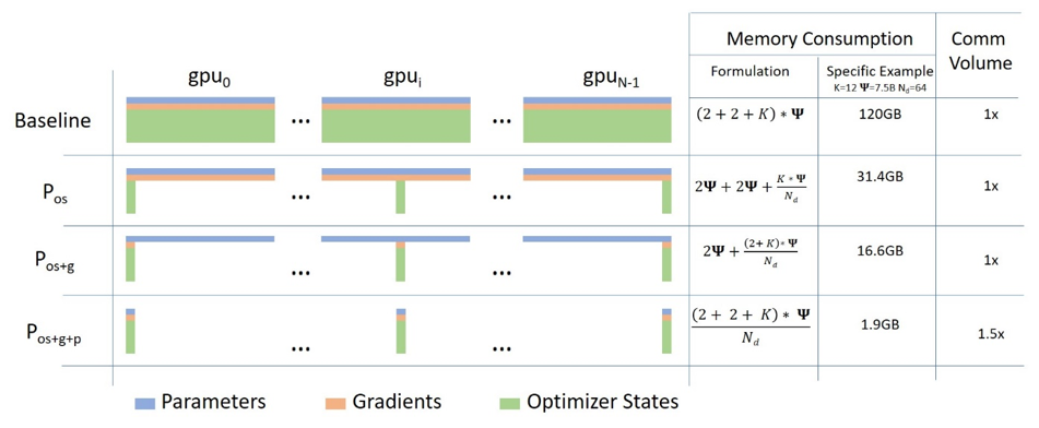
Zero Redundancy Optimizer is a more memory efficient type of data parallelism. It significantly improves memory efficiency by partitioning parameters, gradients, and optimizer states across data parallel processes to reduce memory usage. There are three ZeRO stages:
- Stage 1 partitions the optimizer states
- Stage 2 partitions the optimizer and gradient states
- Stage 3 partitions the optimizer, gradient, and parameters
Model parallelism
Model parallelism distributes a model across multiple GPUs. There are several ways to split a model, but the typical method distributes the model layers across GPUs. On the forward pass, the first GPU processes a batch of data and passes it to the next group of layers on the next GPU. For the backward pass, the data is sent backward from the final layer to the first layer.
Model parallelism is a useful strategy for training models that are too large to fit into the memory of a single GPU. However, GPU utilization is unbalanced because only one GPU is active at a time. Passing results between GPUs also adds communication overhead and it can be a bottleneck.
Pipeline parallelism
Pipeline parallelism is conceptually very similar to model parallelism, but it’s more efficient because it reduces the amount of idle GPU time. Instead of waiting for each GPU to finish processing a batch of data, pipeline parallelism creates micro-batches of data. As soon as one micro-batch is finished, it is passed to the next GPU. This way, each GPU can concurrently process part of the data without waiting for the other GPU to completely finish processing a mini batch of data.
Pipeline parallelism shares the same advantages as model parallelism, but it optimizes GPU utilization and reduces idle time. But pipeline parallelism can be more complex because models may need to be rewritten as a sequence of nn.Sequential modules and it also isn’t possible to completely reduce idle time because the last forward pass must also wait for the backward pass to finish.
Tensor parallelism
Tensor parallelism distributes large tensor computations across multiple GPUs. The tensors are sliced horizontally or vertically and each slice is processed by a separate GPU. Each GPU performs its calculations on its tensor slice and the results are synchronized at the end to reconstruct the final result.
Tensor parallelism is effective for training large models that don’t fit into the memory of a single GPU. It is also faster and more efficient because each GPU can process its tensor slice in parallel, and it can be combined with other parallelism methods. Like other parallelism methods though, tensor parallelism adds communication overhead between GPUs.
Refer to the Tensor parallelism guide to learn how to use it for inference.
Hybrid parallelism
Parallelism methods can be combined to achieve even greater memory savings and more efficiently train models with billions of parameters.
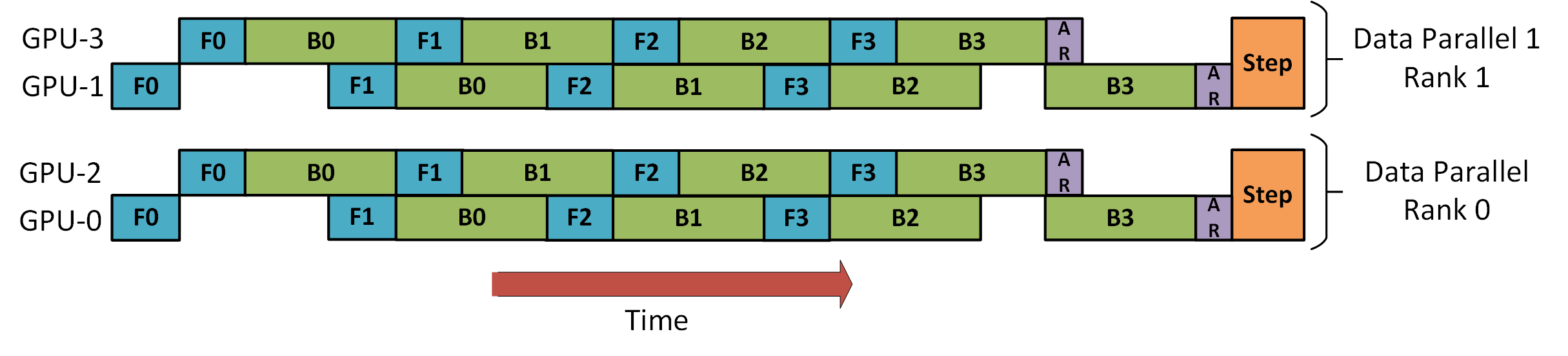
Data parallelism and pipeline parallelism
Data and pipeline parallelism distributes the data across GPUs and divides each mini batch of data into micro-batches to achieve pipeline parallelism.
Each data parallel rank treats the process as if there were only one GPU instead of two, but GPUs 0 and 1 can offload micro-batches of data to GPUs 2 and 3 and reduce idle time.
This approach optimizes parallel data processing by reducing idle GPU utilization.
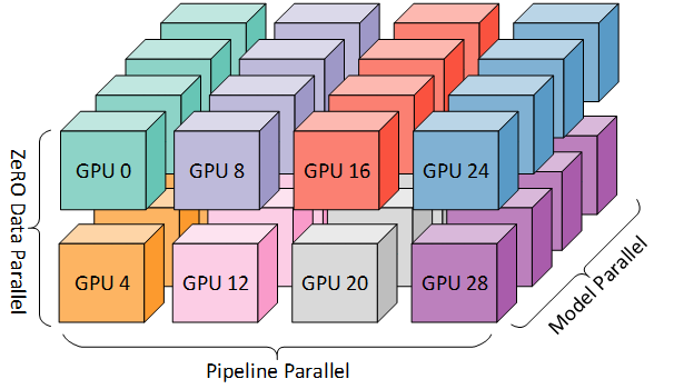
ZeRO data parallelism, pipeline parallelism, and model parallelism (3D parallelism)
Data, pipeline and model parallelism combine to form 3D parallelism to optimize memory and compute efficiency.
Memory efficiency is achieved by splitting the model across GPUs and also dividing it into stages to create a pipeline. This allows GPUs to work in parallel on micro-batches of data, reducing the memory usage of the model, optimizer, and activations.
Compute efficiency is enabled by ZeRO data parallelism where each GPU only stores a slice of the model, optimizer, and activations. This allows higher communication bandwidth between data parallel nodes because communication can occur independently or in parallel with the other pipeline stages.
This approach is scalable to extremely large models with trillions of parameters.