Transformers documentation

Semantic segmentation

Transformers

Join the Hugging Face community

and get access to the augmented documentation experience

Collaborate on models, datasets and Spaces

Faster examples with accelerated inference

Switch between documentation themes

to get started

Semantic segmentation

セマンティックセグメンテーションでは、画像の個々のピクセルにラベルまたはクラスを割り当てます。セグメンテーションにはいくつかのタイプがありますが、セマンティックセグメンテーションの場合、同じオブジェクトの一意のインスタンス間の区別は行われません。両方のオブジェクトに同じラベルが付けられます (たとえば、car-1とcar-2の代わりにcar)。セマンティックセグメンテーションの一般的な現実世界のアプリケーションには、歩行者や重要な交通情報を識別するための自動運転車のトレーニング、医療画像内の細胞と異常の識別、衛星画像からの環境変化の監視などが含まれます。

このガイドでは、次の方法を説明します。

SceneParse150 データセットの SegFormer を微調整します。
微調整したモデルを推論に使用します。

このチュートリアルで説明するタスクは、次のモデルアーキテクチャでサポートされています。

BEiT, Data2VecVision, DPT, MobileNetV2, MobileViT, MobileViTV2, SegFormer, UPerNet

始める前に、必要なライブラリがすべてインストールされていることを確認してください。

pip install -q datasets transformers evaluate

モデルをアップロードしてコミュニティと共有できるように、Hugging Face アカウントにログインすることをお勧めします。プロンプトが表示されたら、トークンを入力してログインします。

>>> from huggingface_hub import notebook_login

>>> notebook_login()

Load SceneParse150 dataset

まず、SceneParse150 データセットの小さいサブセットを 🤗 データセットライブラリから読み込みます。これにより、完全なデータセットのトレーニングにさらに時間を費やす前に、実験してすべてが機能することを確認する機会が得られます。

>>> from datasets import load_dataset

>>> ds = load_dataset("scene_parse_150", split="train[:50]")

train_test_split メソッドを使用して、データセットの train 分割をトレインセットとテストセットに分割します。

>>> ds = ds.train_test_split(test_size=0.2)
>>> train_ds = ds["train"]
>>> test_ds = ds["test"]

次に、例を見てみましょう。

>>> train_ds[0]
{'image': <PIL.JpegImagePlugin.JpegImageFile image mode=RGB size=512x683 at 0x7F9B0C201F90>,
 'annotation': <PIL.PngImagePlugin.PngImageFile image mode=L size=512x683 at 0x7F9B0C201DD0>,
 'scene_category': 368}

image: シーンの PIL イメージ。
annotation: セグメンテーションマップの PIL イメージ。モデルのターゲットでもあります。
scene_category: “kitchen”や”office”などの画像シーンを説明するカテゴリ ID。このガイドでは、imageとannotationのみが必要になります。どちらも PIL イメージです。

また、ラベル ID をラベルクラスにマップする辞書を作成することもできます。これは、後でモデルを設定するときに役立ちます。ハブからマッピングをダウンロードし、id2label および label2id ディクショナリを作成します。

>>> import json
>>> from huggingface_hub import cached_download, hf_hub_url

>>> repo_id = "huggingface/label-files"
>>> filename = "ade20k-id2label.json"
>>> id2label = json.load(open(cached_download(hf_hub_url(repo_id, filename, repo_type="dataset")), "r"))
>>> id2label = {int(k): v for k, v in id2label.items()}
>>> label2id = {v: k for k, v in id2label.items()}
>>> num_labels = len(id2label)

Preprocess

次のステップでは、SegFormer 画像プロセッサをロードして、モデルの画像と注釈を準備します。このデータセットのような一部のデータセットは、バックグラウンドクラスとしてゼロインデックスを使用します。ただし、実際には背景クラスは 150 個のクラスに含まれていないため、reduce_labels=Trueを設定してすべてのラベルから 1 つを引く必要があります。ゼロインデックスは 255 に置き換えられるため、SegFormer の損失関数によって無視されます。

>>> from transformers import AutoImageProcessor

>>> checkpoint = "nvidia/mit-b0"
>>> image_processor = AutoImageProcessor.from_pretrained(checkpoint, reduce_labels=True)

Pytorch

Hide Pytorch content

モデルを過学習に対してより堅牢にするために、画像データセットにいくつかのデータ拡張を適用するのが一般的です。このガイドでは、torchvision の ColorJitter 関数を使用します。 ) を使用して画像の色のプロパティをランダムに変更しますが、任意の画像ライブラリを使用することもできます。

>>> from torchvision.transforms import ColorJitter

>>> jitter = ColorJitter(brightness=0.25, contrast=0.25, saturation=0.25, hue=0.1)

次に、モデルの画像と注釈を準備するための 2 つの前処理関数を作成します。これらの関数は、画像をpixel_valuesに変換し、注釈をlabelsに変換します。トレーニングセットの場合、画像を画像プロセッサに提供する前に jitter が適用されます。テストセットの場合、テスト中にデータ拡張が適用されないため、画像プロセッサはimagesを切り取って正規化し、ラベルのみを切り取ります。

>>> def train_transforms(example_batch):
...     images = [jitter(x) for x in example_batch["image"]]
...     labels = [x for x in example_batch["annotation"]]
...     inputs = image_processor(images, labels)
...     return inputs


>>> def val_transforms(example_batch):
...     images = [x for x in example_batch["image"]]
...     labels = [x for x in example_batch["annotation"]]
...     inputs = image_processor(images, labels)
...     return inputs

データセット全体にjitterを適用するには、🤗 Datasets set_transform 関数を使用します。変換はオンザフライで適用されるため、高速で消費するディスク容量が少なくなります。

>>> train_ds.set_transform(train_transforms)
>>> test_ds.set_transform(val_transforms)

TensorFlow

Hide TensorFlow content

モデルを過学習に対してより堅牢にするために、画像データセットにいくつかのデータ拡張を適用するのが一般的です。このガイドでは、tf.image を使用して画像の色のプロパティをランダムに変更しますが、任意のプロパティを使用することもできます。画像好きな図書館。 2 つの別々の変換関数を定義します。

画像拡張を含むトレーニングデータ変換
🤗 Transformers のコンピュータービジョンモデルはチャネル優先のレイアウトを想定しているため、画像を転置するだけの検証データ変換

>>> import tensorflow as tf


>>> def aug_transforms(image):
...     image = tf.keras.utils.img_to_array(image)
...     image = tf.image.random_brightness(image, 0.25)
...     image = tf.image.random_contrast(image, 0.5, 2.0)
...     image = tf.image.random_saturation(image, 0.75, 1.25)
...     image = tf.image.random_hue(image, 0.1)
...     image = tf.transpose(image, (2, 0, 1))
...     return image


>>> def transforms(image):
...     image = tf.keras.utils.img_to_array(image)
...     image = tf.transpose(image, (2, 0, 1))
...     return image

次に、モデルの画像と注釈のバッチを準備する 2 つの前処理関数を作成します。これらの機能が適用されます画像変換を行い、以前にロードされた image_processor を使用して画像を pixel_values に変換し、 labelsへの注釈。 ImageProcessor は、画像のサイズ変更と正規化も処理します。

>>> def train_transforms(example_batch):
...     images = [aug_transforms(x.convert("RGB")) for x in example_batch["image"]]
...     labels = [x for x in example_batch["annotation"]]
...     inputs = image_processor(images, labels)
...     return inputs


>>> def val_transforms(example_batch):
...     images = [transforms(x.convert("RGB")) for x in example_batch["image"]]
...     labels = [x for x in example_batch["annotation"]]
...     inputs = image_processor(images, labels)
...     return inputs

データセット全体に前処理変換を適用するには、🤗 Datasets set_transform 関数を使用します。変換はオンザフライで適用されるため、高速で消費するディスク容量が少なくなります。

>>> train_ds.set_transform(train_transforms)
>>> test_ds.set_transform(val_transforms)

Evaluate

トレーニング中にメトリクスを含めると、多くの場合、モデルのパフォーマンスを評価するのに役立ちます。 🤗 Evaluate ライブラリを使用して、評価メソッドをすばやくロードできます。このタスクでは、Mean Intersection over Union (IoU) メトリックをロードします (🤗 Evaluate クイックツアーを参照して、メトリクスをロードして計算する方法の詳細を確認してください)。

>>> import evaluate

>>> metric = evaluate.load("mean_iou")

次に、メトリクスを compute する関数を作成します。予測を次のように変換する必要があります最初にロジットを作成し、次に compute を呼び出す前にラベルのサイズに一致するように再形成します。

Pytorch

Hide Pytorch content

>>> import numpy as np
>>> import torch
>>> from torch import nn

>>> def compute_metrics(eval_pred):
...     with torch.no_grad():
...         logits, labels = eval_pred
...         logits_tensor = torch.from_numpy(logits)
...         logits_tensor = nn.functional.interpolate(
...             logits_tensor,
...             size=labels.shape[-2:],
...             mode="bilinear",
...             align_corners=False,
...         ).argmax(dim=1)

...         pred_labels = logits_tensor.detach().cpu().numpy()
...         metrics = metric.compute(
...             predictions=pred_labels,
...             references=labels,
...             num_labels=num_labels,
...             ignore_index=255,
...             reduce_labels=False,
...         )
...         for key, value in metrics.items():
...             if type(value) is np.ndarray:
...                 metrics[key] = value.tolist()
...         return metrics

TensorFlow

Hide TensorFlow content

>>> def compute_metrics(eval_pred):
...     logits, labels = eval_pred
...     logits = tf.transpose(logits, perm=[0, 2, 3, 1])
...     logits_resized = tf.image.resize(
...         logits,
...         size=tf.shape(labels)[1:],
...         method="bilinear",
...     )

...     pred_labels = tf.argmax(logits_resized, axis=-1)
...     metrics = metric.compute(
...         predictions=pred_labels,
...         references=labels,
...         num_labels=num_labels,
...         ignore_index=-1,
...         reduce_labels=image_processor.do_reduce_labels,
...     )

...     per_category_accuracy = metrics.pop("per_category_accuracy").tolist()
...     per_category_iou = metrics.pop("per_category_iou").tolist()

...     metrics.update({f"accuracy_{id2label[i]}": v for i, v in enumerate(per_category_accuracy)})
...     metrics.update({f"iou_{id2label[i]}": v for i, v in enumerate(per_category_iou)})
...     return {"val_" + k: v for k, v in metrics.items()}

これでcompute_metrics関数の準備が整いました。トレーニングをセットアップするときにこの関数に戻ります。

Train

Pytorch

Hide Pytorch content

Trainer を使用したモデルの微調整に慣れていない場合は、ここの基本的なチュートリアルをご覧ください。

これでモデルのトレーニングを開始する準備が整いました。 AutoModelForSemanticSegmentation を使用して SegFormer をロードし、ラベル ID とラベルクラス間のマッピングをモデルに渡します。

>>> from transformers import AutoModelForSemanticSegmentation, TrainingArguments, Trainer

>>> model = AutoModelForSemanticSegmentation.from_pretrained(checkpoint, id2label=id2label, label2id=label2id)

この時点で残っている手順は次の 3 つだけです。

TrainingArguments でトレーニングハイパーパラメータを定義します。 image 列が削除されるため、未使用の列を削除しないことが重要です。 image 列がないと、pixel_values を作成できません。この動作を防ぐには、remove_unused_columns=Falseを設定してください。他に必要なパラメータは、モデルの保存場所を指定する output_dir だけです。 push_to_hub=Trueを設定して、このモデルをハブにプッシュします (モデルをアップロードするには、Hugging Face にサインインする必要があります)。各エポックの終了時に、Trainer は IoU メトリックを評価し、トレーニングチェックポイントを保存します。
トレーニング引数を、モデル、データセット、トークナイザー、データ照合器、および compute_metrics 関数とともに Trainer に渡します。
train() を呼び出してモデルを微調整します。

>>> training_args = TrainingArguments(
...     output_dir="segformer-b0-scene-parse-150",
...     learning_rate=6e-5,
...     num_train_epochs=50,
...     per_device_train_batch_size=2,
...     per_device_eval_batch_size=2,
...     save_total_limit=3,
...     evaluation_strategy="steps",
...     save_strategy="steps",
...     save_steps=20,
...     eval_steps=20,
...     logging_steps=1,
...     eval_accumulation_steps=5,
...     remove_unused_columns=False,
...     push_to_hub=True,
... )

>>> trainer = Trainer(
...     model=model,
...     args=training_args,
...     train_dataset=train_ds,
...     eval_dataset=test_ds,
...     compute_metrics=compute_metrics,
... )

>>> trainer.train()

トレーニングが完了したら、 push_to_hub() メソッドを使用してモデルをハブに共有し、誰もがモデルを使用できるようにします。

>>> trainer.push_to_hub()

TensorFlow

Hide TensorFlow content

Keras を使用したモデルの微調整に慣れていない場合は、まず基本チュートリアルを確認してください。

TensorFlow でモデルを微調整するには、次の手順に従います。

トレーニングのハイパーパラメータを定義し、オプティマイザーと学習率スケジュールを設定します。
事前トレーニングされたモデルをインスタンス化します。
🤗 データセットを tf.data.Dataset に変換します。
モデルをコンパイルします。
コールバックを追加してメトリクスを計算し、モデルを 🤗 Hub にアップロードします
fit() メソッドを使用してトレーニングを実行します。

まず、ハイパーパラメーター、オプティマイザー、学習率スケジュールを定義します。

>>> from transformers import create_optimizer

>>> batch_size = 2
>>> num_epochs = 50
>>> num_train_steps = len(train_ds) * num_epochs
>>> learning_rate = 6e-5
>>> weight_decay_rate = 0.01

>>> optimizer, lr_schedule = create_optimizer(
...     init_lr=learning_rate,
...     num_train_steps=num_train_steps,
...     weight_decay_rate=weight_decay_rate,
...     num_warmup_steps=0,
... )

次に、ラベルマッピングとともに TFAutoModelForSemanticSegmentation を使用して SegFormer をロードし、それをコンパイルします。オプティマイザ。 Transformers モデルにはすべてデフォルトのタスク関連の損失関数があるため、次の場合を除き、損失関数を指定する必要はないことに注意してください。

>>> from transformers import TFAutoModelForSemanticSegmentation

>>> model = TFAutoModelForSemanticSegmentation.from_pretrained(
...     checkpoint,
...     id2label=id2label,
...     label2id=label2id,
... )
>>> model.compile(optimizer=optimizer)  # No loss argument!

to_tf_dataset と DefaultDataCollator を使用して、データセットを tf.data.Dataset 形式に変換します。

>>> from transformers import DefaultDataCollator

>>> data_collator = DefaultDataCollator(return_tensors="tf")

>>> tf_train_dataset = train_ds.to_tf_dataset(
...     columns=["pixel_values", "label"],
...     shuffle=True,
...     batch_size=batch_size,
...     collate_fn=data_collator,
... )

>>> tf_eval_dataset = test_ds.to_tf_dataset(
...     columns=["pixel_values", "label"],
...     shuffle=True,
...     batch_size=batch_size,
...     collate_fn=data_collator,
... )

予測から精度を計算し、モデルを 🤗 ハブにプッシュするには、Keras callbacks を使用します。 compute_metrics 関数を KerasMetricCallback に渡します。そして PushToHubCallback を使用してモデルをアップロードします。

>>> from transformers.keras_callbacks import KerasMetricCallback, PushToHubCallback

>>> metric_callback = KerasMetricCallback(
...     metric_fn=compute_metrics, eval_dataset=tf_eval_dataset, batch_size=batch_size, label_cols=["labels"]
... )

>>> push_to_hub_callback = PushToHubCallback(output_dir="scene_segmentation", tokenizer=image_processor)

>>> callbacks = [metric_callback, push_to_hub_callback]

ついに、モデルをトレーニングする準備が整いました。トレーニングおよび検証データセット、エポック数、モデルを微調整するためのコールバック:

>>> model.fit(
...     tf_train_dataset,
...     validation_data=tf_eval_dataset,
...     callbacks=callbacks,
...     epochs=num_epochs,
... )

おめでとう！モデルを微調整し、🤗 Hub で共有しました。これで推論に使用できるようになりました。

Inference

モデルを微調整したので、それを推論に使用できるようになりました。

推論のために画像をロードします。

>>> image = ds[0]["image"]
>>> image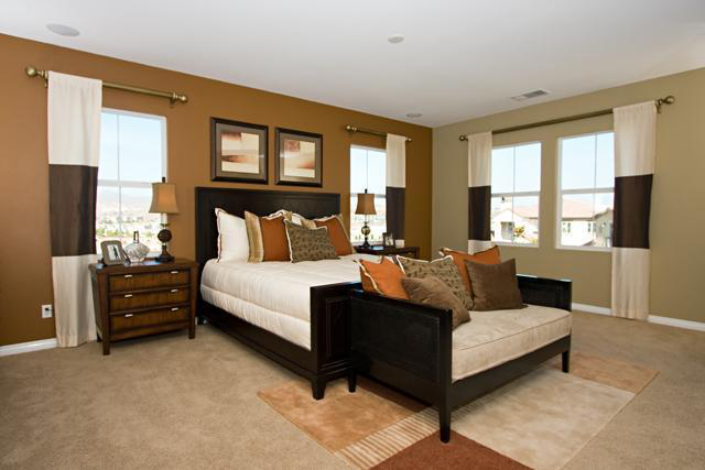

Pytorch

Hide Pytorch content

推論用に微調整されたモデルを試す最も簡単な方法は、それを pipeline() で使用することです。モデルを使用して画像セグメンテーション用の pipelineをインスタンス化し、それに画像を渡します。

>>> from transformers import pipeline

>>> segmenter = pipeline("image-segmentation", model="my_awesome_seg_model")
>>> segmenter(image)
[{'score': None,
  'label': 'wall',
  'mask': <PIL.Image.Image image mode=L size=640x427 at 0x7FD5B2062690>},
 {'score': None,
  'label': 'sky',
  'mask': <PIL.Image.Image image mode=L size=640x427 at 0x7FD5B2062A50>},
 {'score': None,
  'label': 'floor',
  'mask': <PIL.Image.Image image mode=L size=640x427 at 0x7FD5B2062B50>},
 {'score': None,
  'label': 'ceiling',
  'mask': <PIL.Image.Image image mode=L size=640x427 at 0x7FD5B2062A10>},
 {'score': None,
  'label': 'bed ',
  'mask': <PIL.Image.Image image mode=L size=640x427 at 0x7FD5B2062E90>},
 {'score': None,
  'label': 'windowpane',
  'mask': <PIL.Image.Image image mode=L size=640x427 at 0x7FD5B2062390>},
 {'score': None,
  'label': 'cabinet',
  'mask': <PIL.Image.Image image mode=L size=640x427 at 0x7FD5B2062550>},
 {'score': None,
  'label': 'chair',
  'mask': <PIL.Image.Image image mode=L size=640x427 at 0x7FD5B2062D90>},
 {'score': None,
  'label': 'armchair',
  'mask': <PIL.Image.Image image mode=L size=640x427 at 0x7FD5B2062E10>}]

必要に応じて、pipelineの結果を手動で複製することもできます。画像を画像プロセッサで処理し、pixel_values を GPU に配置します。

>>> device = torch.device("cuda" if torch.cuda.is_available() else "cpu")  # use GPU if available, otherwise use a CPU
>>> encoding = image_processor(image, return_tensors="pt")
>>> pixel_values = encoding.pixel_values.to(device)

入力をモデルに渡し、logitsを返します。

>>> outputs = model(pixel_values=pixel_values)
>>> logits = outputs.logits.cpu()

次に、ロジットを元の画像サイズに再スケールします。

>>> upsampled_logits = nn.functional.interpolate(
...     logits,
...     size=image.size[::-1],
...     mode="bilinear",
...     align_corners=False,
... )

>>> pred_seg = upsampled_logits.argmax(dim=1)[0]

TensorFlow

Hide TensorFlow content

画像プロセッサをロードして画像を前処理し、入力を TensorFlow テンソルとして返します。

>>> from transformers import AutoImageProcessor

>>> image_processor = AutoImageProcessor.from_pretrained("MariaK/scene_segmentation")
>>> inputs = image_processor(image, return_tensors="tf")

入力をモデルに渡し、logitsを返します。

>>> from transformers import TFAutoModelForSemanticSegmentation

>>> model = TFAutoModelForSemanticSegmentation.from_pretrained("MariaK/scene_segmentation")
>>> logits = model(**inputs).logits

次に、ロジットを元の画像サイズに再スケールし、クラス次元に argmax を適用します。

>>> logits = tf.transpose(logits, [0, 2, 3, 1])

>>> upsampled_logits = tf.image.resize(
...     logits,
...     # We reverse the shape of `image` because `image.size` returns width and height.
...     image.size[::-1],
... )

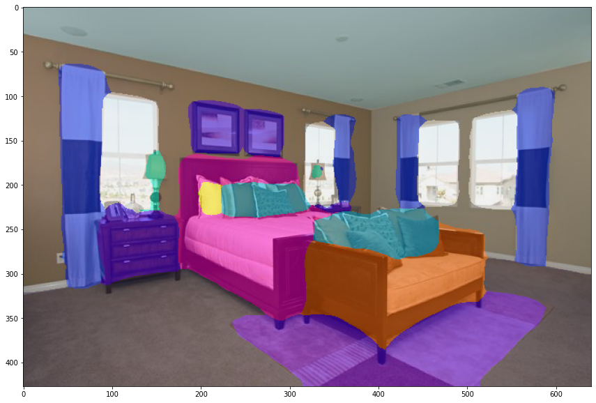
>>> pred_seg = tf.math.argmax(upsampled_logits, axis=-1)[0]

結果を視覚化するには、データセットカラーパレットを、それぞれをマップする ade_palette() としてロードします。クラスを RGB 値に変換します。次に、画像と予測されたセグメンテーションマップを組み合わせてプロットできます。

>>> import matplotlib.pyplot as plt
>>> import numpy as np

>>> color_seg = np.zeros((pred_seg.shape[0], pred_seg.shape[1], 3), dtype=np.uint8)
>>> palette = np.array(ade_palette())
>>> for label, color in enumerate(palette):
...     color_seg[pred_seg == label, :] = color
>>> color_seg = color_seg[..., ::-1]  # convert to BGR

>>> img = np.array(image) * 0.5 + color_seg * 0.5  # plot the image with the segmentation map
>>> img = img.astype(np.uint8)

>>> plt.figure(figsize=(15, 10))
>>> plt.imshow(img)
>>> plt.show()

Image of bedroom overlaid with segmentation map

< > Update on GitHub

←画像分類ビデオの分類→