Evaluate documentation
Using the evaluator
Using the evaluator
The Evaluator classes allow to evaluate a triplet of model, dataset, and metric. The models wrapped in a pipeline, responsible for handling all preprocessing and post-processing and out-of-the-box, Evaluators support transformers pipelines for the supported tasks, but custom pipelines can be passed, as showcased in the section Using the evaluator with custom pipelines.
Currently supported tasks are:
"text-classification": will use the TextClassificationEvaluator."token-classification": will use the TokenClassificationEvaluator."question-answering": will use the QuestionAnsweringEvaluator."image-classification": will use the ImageClassificationEvaluator."text-generation": will use the TextGenerationEvaluator."text2text-generation": will use the Text2TextGenerationEvaluator."summarization": will use the SummarizationEvaluator."translation": will use the TranslationEvaluator."automatic-speech-recognition": will use the AutomaticSpeechRecognitionEvaluator."audio-classification": will use the AudioClassificationEvaluator.
To run an Evaluator with several tasks in a single call, use the EvaluationSuite, which runs evaluations on a collection of SubTasks.
Each task has its own set of requirements for the dataset format and pipeline output, make sure to check them out for your custom use case. Let’s have a look at some of them and see how you can use the evaluator to evalute a single or multiple of models, datasets, and metrics at the same time.
Text classification
The text classification evaluator can be used to evaluate text models on classification datasets such as IMDb. Beside the model, data, and metric inputs it takes the following optional inputs:
input_column="text": with this argument the column with the data for the pipeline can be specified.label_column="label": with this argument the column with the labels for the evaluation can be specified.label_mapping=None: the label mapping aligns the labels in the pipeline output with the labels need for evaluation. E.g. the labels inlabel_columncan be integers (0/1) whereas the pipeline can produce label names such as"positive"/"negative". With that dictionary the pipeline outputs are mapped to the labels.
By default the "accuracy" metric is computed.
Evaluate models on the Hub
There are several ways to pass a model to the evaluator: you can pass the name of a model on the Hub, you can load a transformers model and pass it to the evaluator or you can pass an initialized transformers.Pipeline. Alternatively you can pass any callable function that behaves like a pipeline call for the task in any framework.
So any of the following works:
from datasets import load_dataset
from evaluate import evaluator
from transformers import AutoModelForSequenceClassification, pipeline

data = load_dataset("imdb", split="test").shuffle(seed=42).select(range(1000))
task_evaluator = evaluator("text-classification")

# 1. Pass a model name or path
eval_results = task_evaluator.compute(
    model_or_pipeline="lvwerra/distilbert-imdb",
    data=data,
    label_mapping={"NEGATIVE": 0, "POSITIVE": 1}
)

# 2. Pass an instantiated model
model = AutoModelForSequenceClassification.from_pretrained("lvwerra/distilbert-imdb")

eval_results = task_evaluator.compute(
    model_or_pipeline=model,
    data=data,
    label_mapping={"NEGATIVE": 0, "POSITIVE": 1}
)

# 3. Pass an instantiated pipeline
pipe = pipeline("text-classification", model="lvwerra/distilbert-imdb")

eval_results = task_evaluator.compute(
    model_or_pipeline=pipe,
    data=data,
    label_mapping={"NEGATIVE": 0, "POSITIVE": 1}
)
print(eval_results)
Without specifying a device, the default for model inference will be the first GPU on the machine if one is available, and else CPU. If you want to use a specific device you can pass device to compute where -1 will use the GPU and a positive integer (starting with 0) will use the associated CUDA device.
The results will look as follows:
{
    'accuracy': 0.918,
    'latency_in_seconds': 0.013,
    'samples_per_second': 78.887,
    'total_time_in_seconds': 12.676
}
Note that evaluation results include both the requested metric, and information about the time it took to obtain predictions through the pipeline.
The time performances can give useful indication on model speed for inference but should be taken with a grain of salt: they include all the processing that goes on in the pipeline. This may include tokenizing, post-processing, that may be different depending on the model. Furthermore, it depends a lot on the hardware you are running the evaluation on and you may be able to improve the performance by optimizing things like the batch size.
Evaluate multiple metrics
With the combine() function one can bundle several metrics into an object that behaves like a single metric. We can use this to evaluate several metrics at once with the evaluator:
import evaluate

eval_results = task_evaluator.compute(
    model_or_pipeline="lvwerra/distilbert-imdb",
    data=data,
    metric=evaluate.combine(["accuracy", "recall", "precision", "f1"]),
    label_mapping={"NEGATIVE": 0, "POSITIVE": 1}
)
print(eval_results)
The results will look as follows:
{
    'accuracy': 0.918,
    'f1': 0.916,
    'precision': 0.9147,
    'recall': 0.9187,
    'latency_in_seconds': 0.013,
    'samples_per_second': 78.887,
    'total_time_in_seconds': 12.676
}
Next let’s have a look at token classification.
Token Classification
With the token classification evaluator one can evaluate models for tasks such as NER or POS tagging. It has the following specific arguments:
input_column="text": with this argument the column with the data for the pipeline can be specified.label_column="label": with this argument the column with the labels for the evaluation can be specified.label_mapping=None: the label mapping aligns the labels in the pipeline output with the labels need for evaluation. E.g. the labels inlabel_columncan be integers (0/1) whereas the pipeline can produce label names such as"positive"/"negative". With that dictionary the pipeline outputs are mapped to the labels.join_by=" ": While most datasets are already tokenized the pipeline expects a string. Thus the tokens need to be joined before passing to the pipeline. By default they are joined with a whitespace.
Let’s have a look how we can use the evaluator to benchmark several models.
Benchmarking several models
Here is an example where several models can be compared thanks to the evaluator in only a few lines of code, abstracting away the preprocessing, inference, postprocessing, metric computation:
import pandas as pd
from datasets import load_dataset
from evaluate import evaluator
from transformers import pipeline

models = [
    "xlm-roberta-large-finetuned-conll03-english",
    "dbmdz/bert-large-cased-finetuned-conll03-english",
    "elastic/distilbert-base-uncased-finetuned-conll03-english",
    "dbmdz/electra-large-discriminator-finetuned-conll03-english",
    "gunghio/distilbert-base-multilingual-cased-finetuned-conll2003-ner",
    "philschmid/distilroberta-base-ner-conll2003",
    "Jorgeutd/albert-base-v2-finetuned-ner",
]

data = load_dataset("conll2003", split="validation").shuffle().select(range(1000))
task_evaluator = evaluator("token-classification")

results = []
for model in models:
    results.append(
        task_evaluator.compute(
            model_or_pipeline=model, data=data, metric="seqeval"
            )
        )

df = pd.DataFrame(results, index=models)
df[["overall_f1", "overall_accuracy", "total_time_in_seconds", "samples_per_second", "latency_in_seconds"]]
The result is a table that looks like this:
| model | overall_f1 | overall_accuracy | total_time_in_seconds | samples_per_second | latency_in_seconds |
|---|---|---|---|---|---|
| Jorgeutd/albert-base-v2-finetuned-ner | 0.941 | 0.989 | 4.515 | 221.468 | 0.005 |
| dbmdz/bert-large-cased-finetuned-conll03-english | 0.962 | 0.881 | 11.648 | 85.850 | 0.012 |
| dbmdz/electra-large-discriminator-finetuned-conll03-english | 0.965 | 0.881 | 11.456 | 87.292 | 0.011 |
| elastic/distilbert-base-uncased-finetuned-conll03-english | 0.940 | 0.989 | 2.318 | 431.378 | 0.002 |
| gunghio/distilbert-base-multilingual-cased-finetuned-conll2003-ner | 0.947 | 0.991 | 2.376 | 420.873 | 0.002 |
| philschmid/distilroberta-base-ner-conll2003 | 0.961 | 0.994 | 2.436 | 410.579 | 0.002 |
| xlm-roberta-large-finetuned-conll03-english | 0.969 | 0.882 | 11.996 | 83.359 | 0.012 |
Visualizing results
You can feed in the results list above into the plot_radar() function to visualize different aspects of their performance and choose the model that is the best fit, depending on the metric(s) that are relevant to your use case:
import evaluate
from evaluate.visualization import radar_plot

>>> plot = radar_plot(data=results, model_names=models, invert_range=["latency_in_seconds"])
>>> plot.show()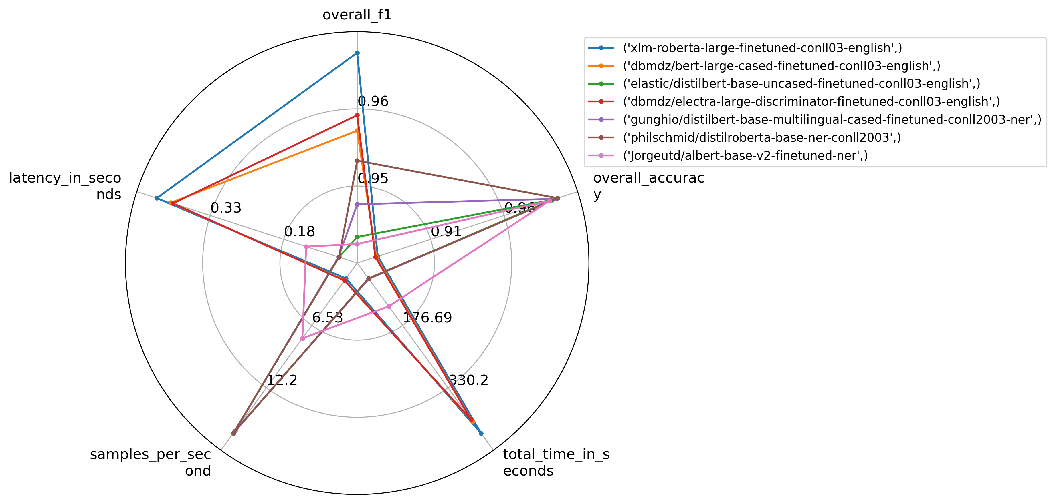
Don’t forget to specify invert_range for metrics for which smaller is better (such as the case for latency in seconds).
If you want to save the plot locally, you can use the plot.savefig() function with the option bbox_inches='tight', to make sure no part of the image gets cut off.
Question Answering
With the question-answering evaluator one can evaluate models for QA without needing to worry about the complicated pre- and post-processing that’s required for these models. It has the following specific arguments:
question_column="question": the name of the column containing the question in the datasetcontext_column="context": the name of the column containing the contextid_column="id": the name of the column cointaing the identification field of the question and answer pairlabel_column="answers": the name of the column containing the answerssquad_v2_format=None: whether the dataset follows the format of squad_v2 dataset where a question may have no answer in the context. If this parameter is not provided, the format will be automatically inferred.
Let’s have a look how we can evaluate QA models and compute confidence intervals at the same time.
Confidence intervals
Every evaluator comes with the options to compute confidence intervals using bootstrapping. Simply pass strategy="bootstrap" and set the number of resanmples with n_resamples.
from datasets import load_dataset
from evaluate import evaluator

task_evaluator = evaluator("question-answering")

data = load_dataset("squad", split="validation[:1000]")
eval_results = task_evaluator.compute(
    model_or_pipeline="distilbert-base-uncased-distilled-squad",
    data=data,
    metric="squad",
    strategy="bootstrap",
    n_resamples=30
)
Results include confidence intervals as well as error estimates as follows:
{
    'exact_match':
    {
        'confidence_interval': (79.67, 84.54),
        'score': 82.30,
        'standard_error': 1.28
    },
    'f1':
    {
        'confidence_interval': (85.30, 88.88),
        'score': 87.23,
        'standard_error': 0.97
    },
    'latency_in_seconds': 0.0085,
    'samples_per_second': 117.31,
    'total_time_in_seconds': 8.52
 }
Image classification
With the image classification evaluator we can evaluate any image classifier. It uses the same keyword arguments at the text classifier:
input_column="image": the name of the column containing the images as PIL ImageFilelabel_column="label": the name of the column containing the labelslabel_mapping=None: We want to map class labels defined by the model in the pipeline to values consistent with those defined in thelabel_column
Let’s have a look at how can evaluate image classification models on large datasets.
Handling large datasets
The evaluator can be used on large datasets! Below, an example shows how to use it on ImageNet-1k for image classification. Beware that this example will require to download ~150 GB.
data = load_dataset("imagenet-1k", split="validation", token=True)

pipe = pipeline(
    task="image-classification",
    model="facebook/deit-small-distilled-patch16-224"
)

task_evaluator = evaluator("image-classification")
eval_results = task_evaluator.compute(
    model_or_pipeline=pipe,
    data=data,
    metric="accuracy",
    label_mapping=pipe.model.config.label2id
)
Since we are using datasets to store data we make use of a technique called memory mappings. This means that the dataset is never fully loaded into memory which saves a lot of RAM. Running the above code only uses roughly 1.5 GB of RAM while the validation split is more than 30 GB big.