Datasets documentation
Depth estimation
Depth estimation
Depth estimation datasets are used to train a model to approximate the relative distance of every pixel in an image from the camera, also known as depth. The applications enabled by these datasets primarily lie in areas like visual machine perception and perception in robotics. Example applications include mapping streets for self-driving cars. This guide will show you how to apply transformations to a depth estimation dataset.
Before you start, make sure you have up-to-date versions of albumentations installed:
pip install -U albumentations
Albumentations is a Python library for performing data augmentation for computer vision. It supports various computer vision tasks such as image classification, object detection, segmentation, and keypoint estimation.
This guide uses the NYU Depth V2 dataset which is comprised of video sequences from various indoor scenes, recorded by RGB and depth cameras. The dataset consists of scenes from 3 cities and provides images along with their depth maps as labels.
Load the train split of the dataset and take a look at an example:
>>> from datasets import load_dataset

>>> train_dataset = load_dataset("sayakpaul/nyu_depth_v2", split="train")
>>> index = 17
>>> example = train_dataset[index]
>>> example
{'image': <PIL.PngImagePlugin.PngImageFile image mode=RGB size=640x480>,
 'depth_map': <PIL.PngImagePlugin.PngImageFile image mode=L size=640x480>}
The dataset has two fields:
image: a PIL image object.depth_map: depth map of the image.
Next, check out an image with:
>>> example["image"]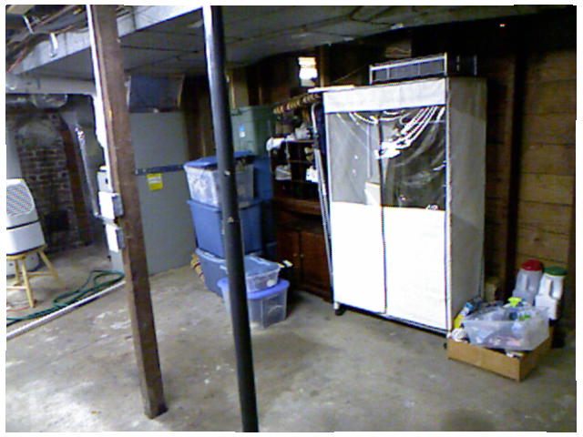
Now take a look at its corresponding depth map:
>>> example["depth_map"]
It’s all black! You’ll need to add some color to the depth map to visualize it properly (the utility below is taken from the FastDepth repository).
>>> import numpy as np
>>> import matplotlib.pyplot as plt

>>> cmap = plt.cm.viridis

>>> def colored_depthmap(depth, d_min=None, d_max=None):
...     if d_min is None:
...         d_min = np.min(depth)
...     if d_max is None:
...         d_max = np.max(depth)
...     depth_relative = (depth - d_min) / (d_max - d_min)
...     return 255 * cmap(depth_relative)[:,:,:3]

>>> def show_depthmap(depth_map):
...    if not isinstance(depth_map, np.ndarray):
...        depth_map = np.array(depth_map)
...    if depth_map.ndim == 3:
...        depth_map = depth_map.squeeze()

...    d_min = np.min(depth_map)
...    d_max = np.max(depth_map)
...    depth_map = colored_depthmap(depth_map, d_min, d_max)

...    plt.imshow(depth_map.astype("uint8"))
...    plt.axis("off")
...    plt.show()

>>> show_depthmap(example["depth_map"])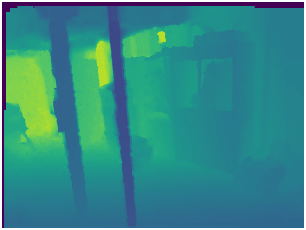
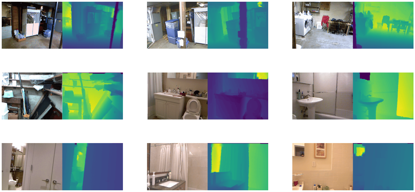
You can also visualize several different images and their corresponding depth maps.
>>> def merge_into_row(input_image, depth_target):
...     if not isinstance(input_image, np.ndarray):
...         input_image = np.array(input_image)
...
...     d_min = np.min(depth_target)
...     d_max = np.max(depth_target)
...     depth_target_col = colored_depthmap(depth_target, d_min, d_max)
...     img_merge = np.hstack([input_image, depth_target_col])
...
...     return img_merge

>>> random_indices = np.random.choice(len(train_dataset), 9).tolist()
>>> plt.figure(figsize=(15, 6))
>>> for i, idx in enumerate(random_indices):
...     example = train_dataset[idx]
...     ax = plt.subplot(3, 3, i + 1)
...     image_viz = merge_into_row(
...         example["image"], example["depth_map"]
...     )
...     plt.imshow(image_viz.astype("uint8"))
...     plt.axis("off")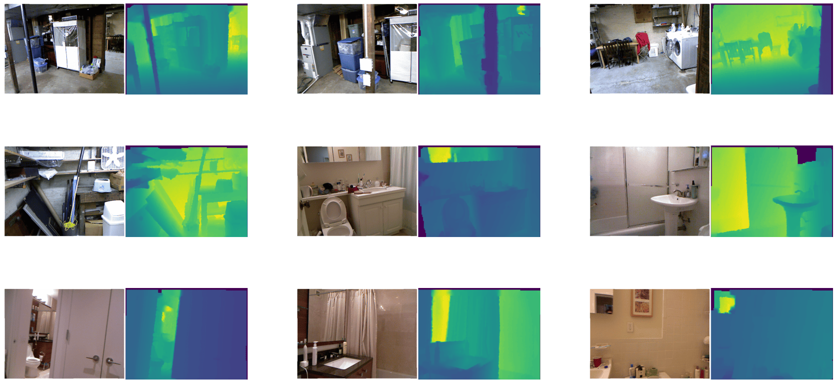
Now apply some augmentations with albumentations. The augmentation transformations include:
- Random horizontal flipping
- Random cropping
- Random brightness and contrast
- Random gamma correction
- Random hue saturation
>>> import albumentations as A

>>> crop_size = (448, 576)
>>> transforms = [
...     A.HorizontalFlip(p=0.5),
...     A.RandomCrop(crop_size[0], crop_size[1]),
...     A.RandomBrightnessContrast(),
...     A.RandomGamma(),
...     A.HueSaturationValue()
... ]
Additionally, define a mapping to better reflect the target key name.
>>> additional_targets = {"depth": "mask"}
>>> aug = A.Compose(transforms=transforms, additional_targets=additional_targets)
With additional_targets defined, you can pass the target depth maps to the depth argument of aug instead of mask. You’ll notice this change
in the apply_transforms() function defined below.
Create a function to apply the transformation to the images as well as their depth maps:
>>> def apply_transforms(examples):
...     transformed_images, transformed_maps = [], []
...     for image, depth_map in zip(examples["image"], examples["depth_map"]):
...         image, depth_map = np.array(image), np.array(depth_map)
...         transformed = aug(image=image, depth=depth_map)
...         transformed_images.append(transformed["image"])
...         transformed_maps.append(transformed["depth"])
...
...     examples["pixel_values"] = transformed_images
...     examples["labels"] = transformed_maps
...     return examples
Use the set_transform() function to apply the transformation on-the-fly to batches of the dataset to consume less disk space:
>>> train_dataset.set_transform(apply_transforms)You can verify the transformation worked by indexing into the pixel_values and labels of an example image:
>>> example = train_dataset[index]

>>> plt.imshow(example["pixel_values"])
>>> plt.axis("off")
>>> plt.show()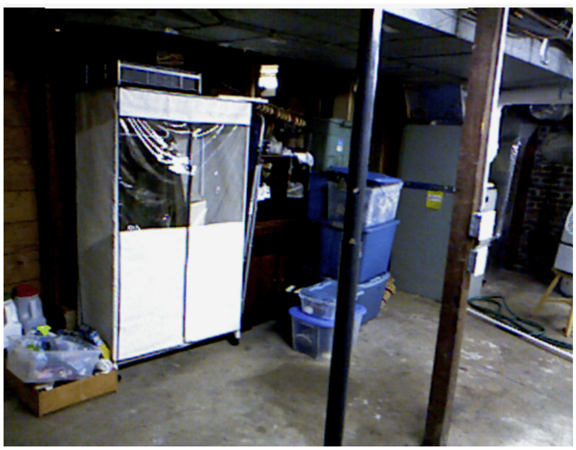
Visualize the same transformation on the image’s corresponding depth map:
>>> show_depthmap(example["labels"])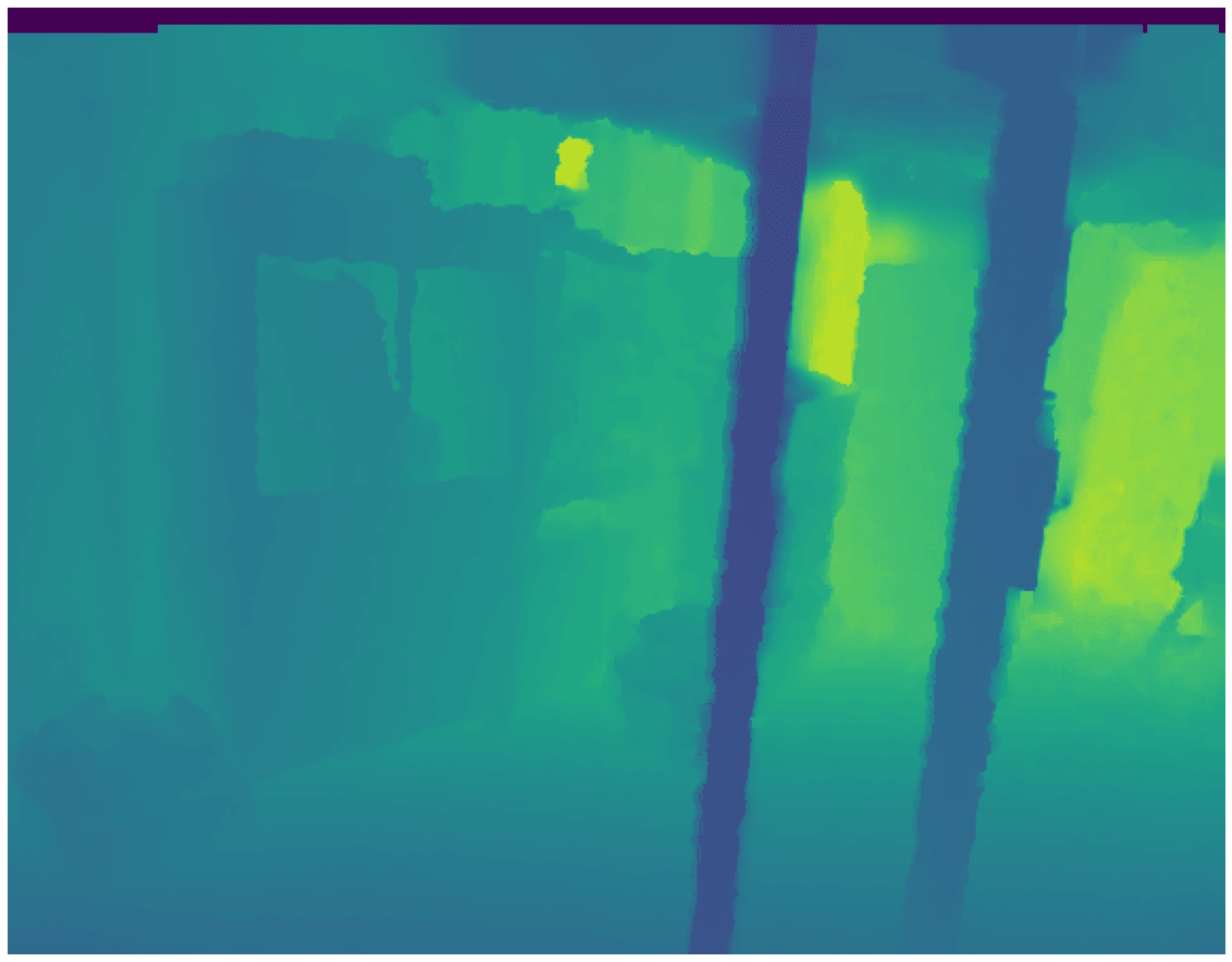
You can also visualize multiple training samples reusing the previous random_indices:
>>> plt.figure(figsize=(15, 6))

>>> for i, idx in enumerate(random_indices):
...     ax = plt.subplot(3, 3, i + 1)
...     example = train_dataset[idx]
...     image_viz = merge_into_row(
...         example["pixel_values"], example["labels"]
...     )
...     plt.imshow(image_viz.astype("uint8"))
...     plt.axis("off")