ovrawm/t_metatime.txt

#!/usr/bin/env python
# coding: utf-8

# # Celltype auto annotation with MetaTiME
# 
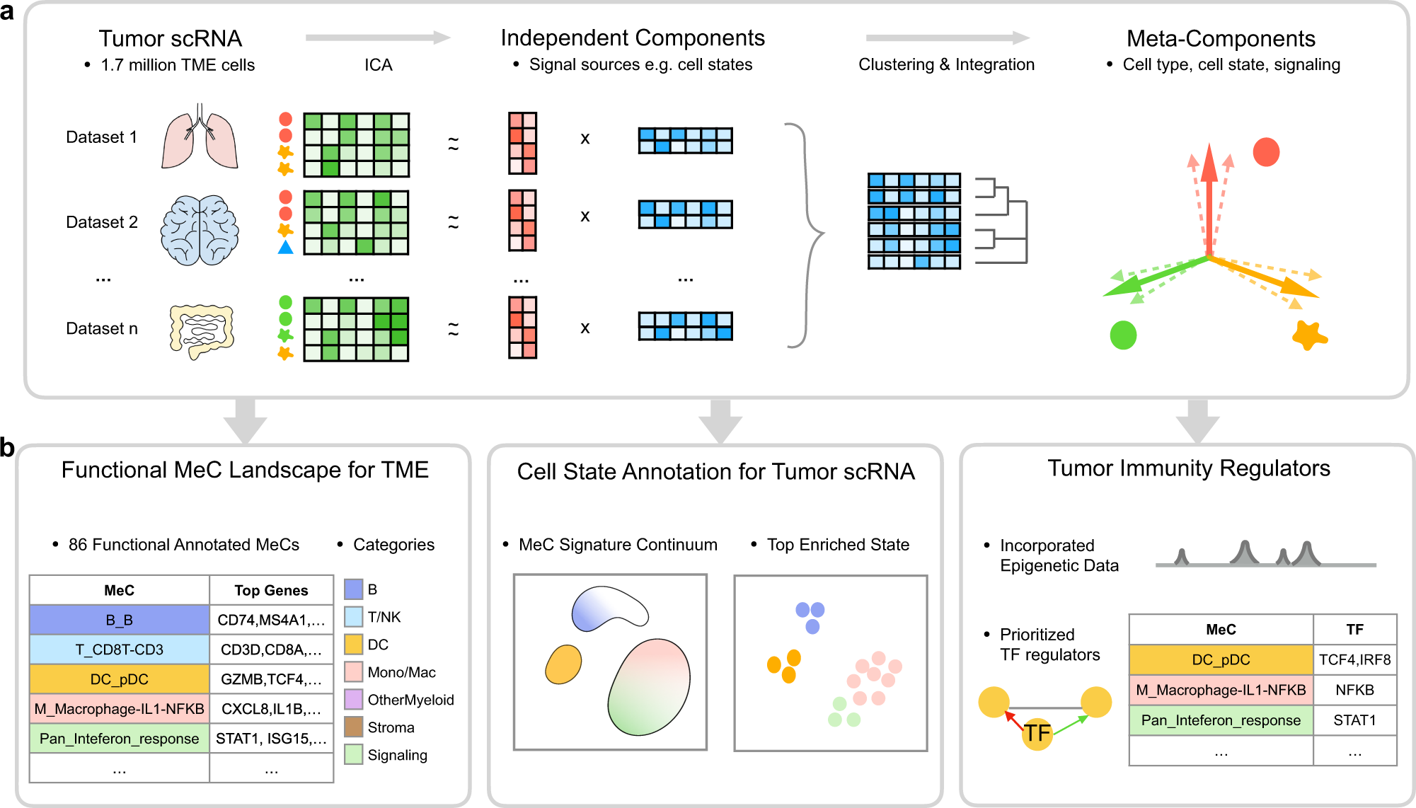
# MetaTiME learns data-driven, interpretable, and reproducible gene programs by integrating millions of single cells from hundreds of tumor scRNA-seq data. The idea is to learn a map of single-cell space with biologically meaningful directions from large-scale data, which helps understand functional cell states and transfers knowledge to new data analysis. MetaTiME provides pretrained meta-components (MeCs) to automatically annotate fine-grained cell states and plot signature continuum for new single-cells of tumor microenvironment.
# 
# Here, we integrate MetaTiME in omicverse. This tutorial demonstrates how to use [MetaTiME (original code)](https://github.com/yi-zhang/MetaTiME/blob/main/docs/notebooks/metatime_annotator.ipynb) to annotate celltype in TME
# 
# Paper: [MetaTiME integrates single-cell gene expression to characterize the meta-components of the tumor immune microenvironment](https://www.nature.com/articles/s41467-023-38333-8)
# 
# Code: https://github.com/yi-zhang/MetaTiME
# 
# Colab_Reproducibility：https://colab.research.google.com/drive/1isvjTfSFM2cy6GzHWAwbuvSjveEJijzP?usp=sharing
# 
# ![metatime](https://media.springernature.com/full/springer-static/image/art%3A10.1038%2Fs41467-023-38333-8/MediaObjects/41467_2023_38333_Fig1_HTML.png)

# In[1]:


import omicverse as ov
ov.utils.ov_plot_set()


# ## Data normalize and Batch remove
# 
# The sample data has multiple patients , and we can use batch correction on patients. Here, we using [scVI](https://docs.scvi-tools.org/en/stable/) to remove batch.
# 
# <div class="admonition warning">
#   <p class="admonition-title">Note</p>
#   <p>
#     If your data contains count matrix, we provide a wrapped function for pre-processing the data. Otherwise, if the data is already depth-normalized, log-transformed, and cells are filtered, we can skip this step.
#   </p>
# </div>

# In[ ]:


'''
import scvi
scvi.model.SCVI.setup_anndata(adata, layer="counts", batch_key="patient")
vae = scvi.model.SCVI(adata, n_layers=2, n_latent=30, gene_likelihood="nb")
vae.train()
adata.obsm["X_scVI"] = vae.get_latent_representation()
'''


# Example data can be obtained from figshare: https://figshare.com/ndownloader/files/41440050

# In[2]:


import scanpy as sc
adata=sc.read('TiME_adata_scvi.h5ad')
adata


# It is recommended that malignant cells are identified first and removed for best practice in cell state annotation.
# 
# In the BCC data, the cluster of malignant cells are identified with `inferCNV`. We can use the pre-saved column 'isTME' to keep Tumor Microenvironment cells.
# 
# These are the authors' exact words, but tests have found that the difference in annotation effect is not that great even without removing the malignant cells
# 
# But I think this step is not necessary

# In[3]:


#adata = adata[adata.obs['isTME']]


# ## Neighborhood graph calculated
# 
# We note that scVI was used earlier to remove the batch effect from the data, so we need to recalculate the neighbourhood map based on what is stored in `adata.obsm['X_scVI']`. Note that if you are not using scVI but using another method to calculate the neighbourhood map, such as `X_pca`, then you need to change `X_scVI` to `X_pca` to complete the calculation
# 
# ```
# #Example
# #sc.tl.pca(adata)
# #sc.pp.neighbors(adata, use_rep="X_pca")
# ```

# In[4]:


sc.pp.neighbors(adata, use_rep="X_scVI")


# To visualize the PCA’s embeddings, we use the `pymde` package wrapper in omicverse. This is an alternative to UMAP that is GPU-accelerated.

# In[5]:


adata.obsm["X_mde"] = ov.utils.mde(adata.obsm["X_scVI"])


# In[6]:


sc.pl.embedding(
    adata,
    basis="X_mde",
    color=["patient"],
    frameon=False,
    ncols=1,
)


# In[7]:


#adata.write_h5ad('adata_mde.h5ad',compression='gzip')
#adata=sc.read('adata_mde.h5ad')


# ## MeteTiME model init
# 
# Next, let's load the pre-computed MetaTiME MetaComponents (MeCs), and their functional annotation.

# In[8]:


TiME_object=ov.single.MetaTiME(adata,mode='table')


# We can over-cluster the cells which is useful for fine-grained cell state annotation.
# 
# As the resolution gets larger, the number of clusters gets larger

# In[9]:


TiME_object.overcluster(resolution=8,clustercol = 'overcluster',)


# ## TME celltype predicted
# 
# We using `TiME_object.predictTiME()` to predicted the latent celltype in TME. 
# 
# - The minor celltype will be stored in `adata.obs['MetaTiME']`
# - The major celltype will be stored in `adata.obs['Major_MetaTiME']`

# In[10]:


TiME_object.predictTiME(save_obs_name='MetaTiME')


# ## Visualize
# 
# The original author provides a drawing function that effectively avoids overlapping labels. Here I have expanded its parameters so that it can be visualised using parameters other than X_umap

# In[13]:


fig,ax=TiME_object.plot(cluster_key='MetaTiME',basis='X_mde',dpi=80)
#fig.save


# We can also use `sc.pl.embedding` to visualize the celltype

# In[15]:


sc.pl.embedding(
    adata,
    basis="X_mde",
    color=["Major_MetaTiME"],
    frameon=False,
    ncols=1,
)


# In[ ]: