微调掩码语言模型

对于许多涉及 Transformer 模型的 NLP 程序, 你可以简单地从 Hugging Face Hub 中获取一个预训练的模型, 然后直接在你的数据上对其进行微调, 以完成手头的任务。只要用于预训练的语料库与用于微调的语料库没有太大区别, 迁移学习通常会产生很好的结果。
但是, 在某些情况下, 你需要先微调数据上的语言模型, 然后再训练特定于任务的head。例如, 如果您的数据集包含法律合同或科学文章, 像 BERT 这样的普通 Transformer 模型通常会将您语料库中的特定领域词视为稀有标记, 结果性能可能不尽如人意。通过在域内数据上微调语言模型, 你可以提高许多下游任务的性能, 这意味着您通常只需执行一次此步骤!
这种在域内数据上微调预训练语言模型的过程通常称为 领域适应。 它于 2018 年由 ULMFiT推广, 这是使迁移学习真正适用于 NLP 的首批神经架构之一 (基于 LSTM)。 下图显示了使用 ULMFiT 进行域自适应的示例; 在本节中, 我们将做类似的事情, 但使用的是 Transformer 而不是 LSTM!


在本节结束时, 你将在Hub上拥有一个掩码语言模型(masked language model), 该模型可以自动完成句子, 如下所示:
让我们开始吧!
🙋 如果您对“掩码语言建模”和“预训练模型”这两个术语感到陌生, 请查看第一章, 我们在其中解释了所有这些核心概念, 并附有视频!
选择用于掩码语言建模的预训练模型
首先, 让我们为掩码语言建模选择一个合适的预训练模型。如以下屏幕截图所示, 你可以通过在Hugging Face Hub上应用”Fill-Mask”过滤器找到:
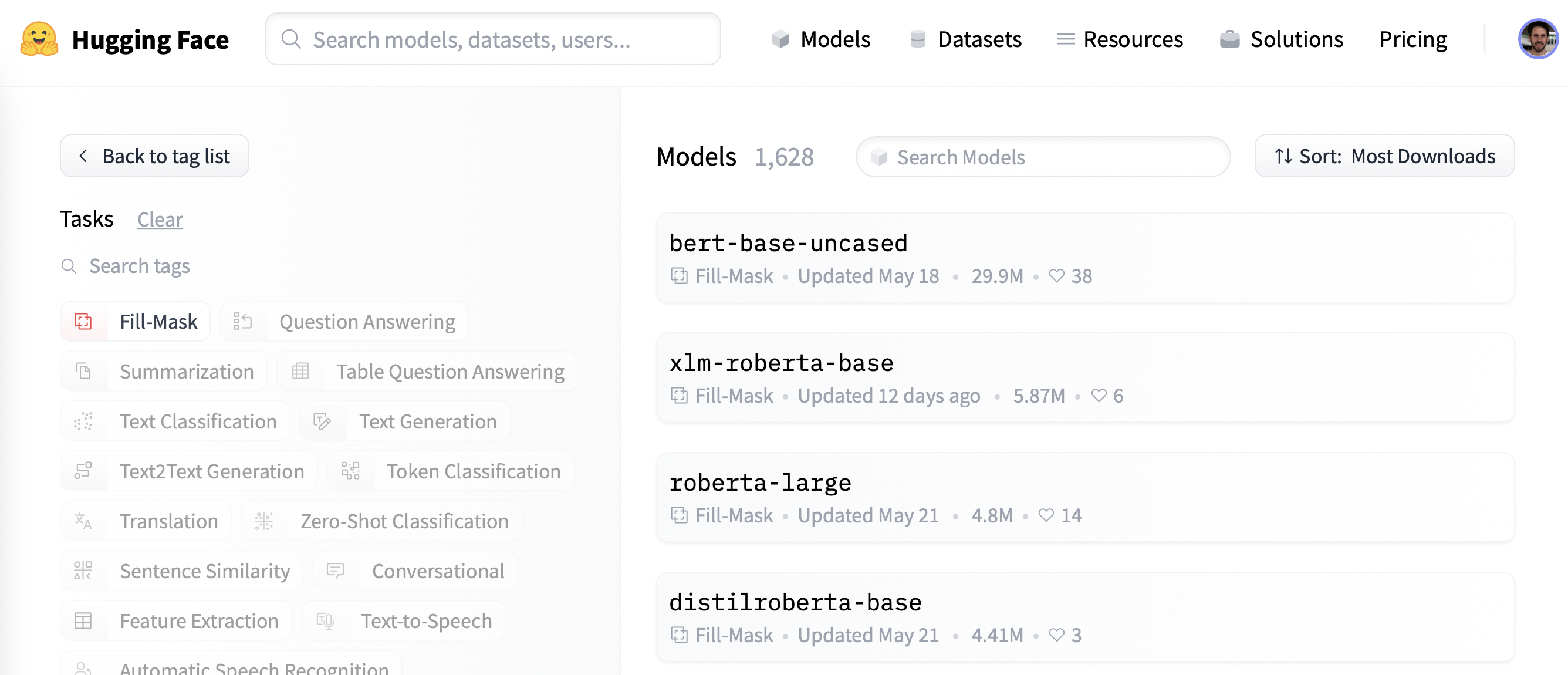
尽管 BERT 和 RoBERTa 系列模型的下载量最大, 但我们将使用名为 DistilBERT的模型。 可以更快地训练, 而下游性能几乎没有损失。这个模型使用一种称为知识蒸馏的特殊技术进行训练, 其中使用像 BERT 这样的大型“教师模型”来指导参数少得多的“学生模型”的训练。在本节中对知识蒸馏细节的解释会使我们离题太远, 但如果你有兴趣, 可以阅读所有相关内容 Natural Language Processing with Transformers (俗称Transformers教科书)。
让我们继续, 使用 AutoModelForMaskedLM 类下载 DistilBERT:
from transformers import AutoModelForMaskedLM

model_checkpoint = "distilbert-base-uncased"
model = AutoModelForMaskedLM.from_pretrained(model_checkpoint)
我们可以通过调用 num_parameters() 方法查看模型有多少参数:
distilbert_num_parameters = model.num_parameters() / 1_000_000
print(f"'>>> DistilBERT number of parameters: {round(distilbert_num_parameters)}M'")
print(f"'>>> BERT number of parameters: 110M'")'>>> DistilBERT number of parameters: 67M'
'>>> BERT number of parameters: 110M'DistilBERT 大约有 6700 万个参数, 大约比 BERT 基本模型小两倍, 这大致意味着训练的速度提高了两倍 — 非常棒! 现在让我们看看这个模型预测什么样的标记最有可能完成一小部分文本:
text = "This is a great [MASK]."作为人类, 我们可以想象 [MASK] 标记有很多可能性, 例如 “day”、 “ride” 或者 “painting”。对于预训练模型, 预测取决于模型所训练的语料库, 因为它会学习获取数据中存在的统计模式。与 BERT 一样, DistilBERT 在English Wikipedia 和 BookCorpus 数据集上进行预训练, 所以我们期望对 [MASK] 的预测能够反映这些领域。为了预测掩码, 我们需要 DistilBERT 的标记器来生成模型的输入, 所以让我们也从 Hub 下载它:
from transformers import AutoTokenizer

tokenizer = AutoTokenizer.from_pretrained(model_checkpoint)
使用标记器和模型, 我们现在可以将我们的文本示例传递给模型, 提取 logits, 并打印出前 5 个候选:
import torch

inputs = tokenizer(text, return_tensors="pt")
token_logits = model(**inputs).logits
# Find the location of [MASK] and extract its logits
mask_token_index = torch.where(inputs["input_ids"] == tokenizer.mask_token_id)[1]
mask_token_logits = token_logits[0, mask_token_index, :]
# Pick the [MASK] candidates with the highest logits
top_5_tokens = torch.topk(mask_token_logits, 5, dim=1).indices[0].tolist()

for token in top_5_tokens:
print(f"'>>> {text.replace(tokenizer.mask_token, tokenizer.decode([token]))}'")'>>> This is a great deal.'
'>>> This is a great success.'
'>>> This is a great adventure.'
'>>> This is a great idea.'
'>>> This is a great feat.'我们可以从输出中看到模型的预测是指日常用语, 鉴于英语维基百科的基础, 这也许并不奇怪。让我们看看我们如何将这个领域改变为更小众的东西 — 高度两极分化的电影评论!
数据集
为了展示域适配, 我们将使用著名的大型电影评论数据集(Large Movie Review Dataset) (或者简称为IMDb), 这是一个电影评论语料库, 通常用于对情感分析模型进行基准测试。通过在这个语料库上对 DistilBERT 进行微调, 我们预计语言模型将根据维基百科的事实数据调整其词汇表, 这些数据已经预先训练到电影评论中更主观的元素。我们可以使用🤗 Datasets中的load_dataset()函数从Hugging Face 中获取数据:
from datasets import load_dataset

imdb_dataset = load_dataset("imdb")
imdb_datasetDatasetDict({
train: Dataset({
features: ['text', 'label'],
num_rows: 25000
})
test: Dataset({
features: ['text', 'label'],
num_rows: 25000
})
unsupervised: Dataset({
features: ['text', 'label'],
num_rows: 50000
})
})我们可以看到 train 和 test 每个拆分包含 25,000 条评论, 而有一个未标记的拆分称为 unsupervised 包含 50,000 条评论。让我们看一些示例, 以了解我们正在处理的文本类型。正如我们在本课程的前几章中所做的那样, 我们将链接 Dataset.shuffle() 和 Dataset.select() 函数创建随机样本:
sample = imdb_dataset["train"].shuffle(seed=42).select(range(3))

for row in sample:
    print(f"\n'>>> Review: {row['text']}'")
    print(f"'>>> Label: {row['label']}'")
'>>> Review: This is your typical Priyadarshan movie--a bunch of loony characters out on some silly mission. His signature climax has the entire cast of the film coming together and fighting each other in some crazy moshpit over hidden money. Whether it is a winning lottery ticket in Malamaal Weekly, black money in Hera Pheri, "kodokoo" in Phir Hera Pheri, etc., etc., the director is becoming ridiculously predictable. Don\'t get me wrong; as clichéd and preposterous his movies may be, I usually end up enjoying the comedy. However, in most his previous movies there has actually been some good humor, (Hungama and Hera Pheri being noteworthy ones). Now, the hilarity of his films is fading as he is using the same formula over and over again.<br /><br />Songs are good. Tanushree Datta looks awesome. Rajpal Yadav is irritating, and Tusshar is not a whole lot better. Kunal Khemu is OK, and Sharman Joshi is the best.'
'>>> Label: 0'

'>>> Review: Okay, the story makes no sense, the characters lack any dimensionally, the best dialogue is ad-libs about the low quality of movie, the cinematography is dismal, and only editing saves a bit of the muddle, but Sam" Peckinpah directed the film. Somehow, his direction is not enough. For those who appreciate Peckinpah and his great work, this movie is a disappointment. Even a great cast cannot redeem the time the viewer wastes with this minimal effort.<br /><br />The proper response to the movie is the contempt that the director San Peckinpah, James Caan, Robert Duvall, Burt Young, Bo Hopkins, Arthur Hill, and even Gig Young bring to their work. Watch the great Peckinpah films. Skip this mess.'
'>>> Label: 0'

'>>> Review: I saw this movie at the theaters when I was about 6 or 7 years old. I loved it then, and have recently come to own a VHS version. <br /><br />My 4 and 6 year old children love this movie and have been asking again and again to watch it. <br /><br />I have enjoyed watching it again too. Though I have to admit it is not as good on a little TV.<br /><br />I do not have older children so I do not know what they would think of it. <br /><br />The songs are very cute. My daughter keeps singing them over and over.<br /><br />Hope this helps.'
'>>> Label: 1'
是的, 这些肯定是电影评论, 如果你年龄足够,你甚至可能会理解上次评论中关于拥有 VHS 版本的评论😜! 虽然我们不需要语言建模的标签, 但我们已经可以看到 0 表示负面评论, 而 1 对应正面。
✏️ 试试看! 创建 无监督 拆分的随机样本, 并验证标签既不是 0 也不是 1。在此过程中, 你还可以检查 train 和 test 拆分中的标签是否确实为 0 或 1 — 这是每个 NLP 从业者在新项目开始时都应该执行的有用的健全性检查!
现在我们已经快速浏览了数据, 让我们深入研究为掩码语言建模做准备。正如我们将看到的, 与我们在第三章中看到的序列分类任务相比, 还需要采取一些额外的步骤。让我们继续!
预处理数据
对于自回归和掩码语言建模, 一个常见的预处理步骤是连接所有示例, 然后将整个语料库拆分为相同大小的块。 这与我们通常的方法完全不同, 我们只是简单地标记单个示例。为什么要将所有内容连接在一起? 原因是单个示例如果太长可能会被截断, 这将导致丢失可能对语言建模任务有用的信息!
因此, 我们将像往常一样首先标记我们的语料库, 但是 没有 在我们的标记器中设置 truncation=True 选项。 我们还将获取可用的单词 ID ((如果我们使用快速标记器, 它们是可用的, 如 第六章中所述), 因为我们稍后将需要它们来进行全字屏蔽。我们将把它包装在一个简单的函数中, 当我们在做的时候, 我们将删除 text 和 label 列, 因为我们不再需要它们:
def tokenize_function(examples):
    result = tokenizer(examples["text"])
    if tokenizer.is_fast:
        result["word_ids"] = [result.word_ids(i) for i in range(len(result["input_ids"]))]
    return result


# Use batched=True to activate fast multithreading!
tokenized_datasets = imdb_dataset.map(
    tokenize_function, batched=True, remove_columns=["text", "label"]
)
tokenized_datasetsDatasetDict({
train: Dataset({
features: ['attention_mask', 'input_ids', 'word_ids'],
num_rows: 25000
})
test: Dataset({
features: ['attention_mask', 'input_ids', 'word_ids'],
num_rows: 25000
})
unsupervised: Dataset({
features: ['attention_mask', 'input_ids', 'word_ids'],
num_rows: 50000
})
})由于 DistilBERT 是一个类似 BERT 的模型, 我们可以看到编码文本由我们在其他章节中看到的 input_ids 和 attention_mask 组成, 以及我们添加的 word_ids。
现在我们已经标记了我们的电影评论, 下一步是将它们组合在一起并将结果分成块。 但是这些块应该有多大? 这最终将取决于你可用的 GPU 内存量, 但一个好的起点是查看模型的最大上下文大小是多少。这可以通过检查标记器的 model_max_length 属性来判断:
tokenizer.model_max_length
512该值来自于与检查点相关联的 tokenizer_config.json 文件; 在这种情况下, 我们可以看到上下文大小是 512 个标记, 就像 BERT 一样。
✏️ 试试看! 一些 Transformer 模型, 例如 BigBird 和 Longformer, 它们具有比BERT和其他早期Transformer模型更长的上下文长度。为这些检查点之一实例化标记器, 并验证 model_max_length 是否与模型卡上引用的内容一致。
因此, 以便在像Google Colab 那样的 GPU 上运行我们的实验, 我们将选择可以放入内存的更小一些的东西:
chunk_size = 128请注意, 在实际场景中使用较小的块大小可能是有害的, 因此你应该使用与将应用模型的用例相对应的大小。
有趣的来了。为了展示串联是如何工作的, 让我们从我们的标记化训练集中取一些评论并打印出每个评论的标记数量:
# Slicing produces a list of lists for each feature
tokenized_samples = tokenized_datasets["train"][:3]

for idx, sample in enumerate(tokenized_samples["input_ids"]):
print(f"'>>> Review {idx} length: {len(sample)}'")'>>> Review 0 length: 200'
'>>> Review 1 length: 559'
'>>> Review 2 length: 192'然后我们可以用一个简单的字典理解来连接所有例子, 如下所示:
concatenated_examples = {
    k: sum(tokenized_samples[k], []) for k in tokenized_samples.keys()
}
total_length = len(concatenated_examples["input_ids"])
print(f"'>>> Concatenated reviews length: {total_length}'")'>>> Concatenated reviews length: 951'很棒, 总长度检查出来了 — 现在, 让我们将连接的评论拆分为大小为 block_size 的块。为此, 我们迭代了 concatenated_examples 中的特征, 并使用列表理解来创建每个特征的切片。结果是每个特征的块字典:
chunks = {
    k: [t[i : i + chunk_size] for i in range(0, total_length, chunk_size)]
    for k, t in concatenated_examples.items()
}

for chunk in chunks["input_ids"]:
print(f"'>>> Chunk length: {len(chunk)}'")'>>> Chunk length: 128'
'>>> Chunk length: 128'
'>>> Chunk length: 128'
'>>> Chunk length: 128'
'>>> Chunk length: 128'
'>>> Chunk length: 128'
'>>> Chunk length: 128'
'>>> Chunk length: 55'正如你在这个例子中看到的, 最后一个块通常会小于最大块大小。有两种主要的策略来处理这个问题:
- 如果最后一个块小于
chunk_size, 请删除它。 - 填充最后一个块, 直到其长度等于
chunk_size。
我们将在这里采用第一种方法, 因此让我们将上述所有逻辑包装在一个函数中, 我们可以将其应用于我们的标记化数据集:
def group_texts(examples):
    # Concatenate all texts
    concatenated_examples = {k: sum(examples[k], []) for k in examples.keys()}
    # Compute length of concatenated texts
    total_length = len(concatenated_examples[list(examples.keys())[0]])
    # We drop the last chunk if it's smaller than chunk_size
    total_length = (total_length // chunk_size) * chunk_size
    # Split by chunks of max_len
    result = {
        k: [t[i : i + chunk_size] for i in range(0, total_length, chunk_size)]
        for k, t in concatenated_examples.items()
    }
    # Create a new labels column
    result["labels"] = result["input_ids"].copy()
    return result
注意, 在 group_texts() 的最后一步中, 我们创建了一个新的 labels 列, 它是 input_ids 列的副本。我们很快就会看到, 这是因为在掩码语言建模中, 目标是预测输入批次中随机掩码的标记, 并通过创建一个 labels 列, 们为我们的语言模型提供了基础事实以供学习。
现在, 让我们使用我们可信赖的 Dataset.map() 函数将 group_texts() 应用到我们的标记化数据集:
lm_datasets = tokenized_datasets.map(group_texts, batched=True)
lm_datasetsDatasetDict({
train: Dataset({
features: ['attention_mask', 'input_ids', 'labels', 'word_ids'],
num_rows: 61289
})
test: Dataset({
features: ['attention_mask', 'input_ids', 'labels', 'word_ids'],
num_rows: 59905
})
unsupervised: Dataset({
features: ['attention_mask', 'input_ids', 'labels', 'word_ids'],
num_rows: 122963
})
})你可以看到, 对文本进行分组, 然后对文本进行分块, 产生的示例比我们最初的 25,000 用于 train和 test 拆分的示例多得多。那是因为我们现在有了涉及 连续标记 的示例, 这些示例跨越了原始语料库中的多个示例。你可以通过在其中一个块中查找特殊的 [SEP] 和 [CLS] 标记来明确的看到这一点:
tokenizer.decode(lm_datasets["train"][1]["input_ids"])".... at.......... high. a classic line : inspector : i'm here to sack one of your teachers. student : welcome to bromwell high. i expect that many adults of my age think that bromwell high is far fetched. what a pity that it isn't! [SEP] [CLS] homelessness ( or houselessness as george carlin stated ) has been an issue for years but never a plan to help those on the street that were once considered human who did everything from going to school, work, or vote for the matter. most people think of the homeless"在此示例中, 你可以看到两篇重叠的电影评论, 一篇关于高中电影, 另一篇关于无家可归。 让我们也看看掩码语言建模的标签是什么样的:
tokenizer.decode(lm_datasets["train"][1]["labels"])".... at.......... high. a classic line : inspector : i'm here to sack one of your teachers. student : welcome to bromwell high. i expect that many adults of my age think that bromwell high is far fetched. what a pity that it isn't! [SEP] [CLS] homelessness ( or houselessness as george carlin stated ) has been an issue for years but never a plan to help those on the street that were once considered human who did everything from going to school, work, or vote for the matter. most people think of the homeless"正如前面的 group_texts() 函数所期望的那样, 这看起来与解码后的 input_ids 相同 — 但是我们的模型怎么可能学到任何东西呢? 我们错过了一个关键步骤: 在输入中的随机位置插入 [MASK] 标记! 让我们看看如何使用特殊的数据整理器在微调期间即时执行此操作。
使用 Trainer API 微调DistilBERT
微调屏蔽语言模型几乎与微调序列分类模型相同, 就像我们在 第三章所作的那样。 唯一的区别是我们需要一个特殊的数据整理器, 它可以随机屏蔽每批文本中的一些标记。幸运的是, 🤗 Transformers 为这项任务准备了专用的 DataCollatorForLanguageModeling 。我们只需要将它转递给标记器和一个 mlm_probability 参数, 该参数指定要屏蔽的标记的分数。我们将选择 15%, 这是 BERT 使用的数量也是文献中的常见选择:
from transformers import DataCollatorForLanguageModeling

data_collator = DataCollatorForLanguageModeling(tokenizer=tokenizer, mlm_probability=0.15)
要了解随机掩码的工作原理, 让我们向数据整理器提供一些示例。由于它需要一个 dict 的列表, 其中每个 dict 表示单个连续文本块, 我们首先迭代数据集, 然后再将批次提供给整理器。我们删除了这个数据整理器的 "word_ids" 键, 因为它不需要它:
samples = [lm_datasets["train"][i] for i in range(2)]
for sample in samples:
    _ = sample.pop("word_ids")

for chunk in data_collator(samples)["input_ids"]:
print(f"\n'>>> {tokenizer.decode(chunk)}'")'>>> [CLS] bromwell [MASK] is a cartoon comedy. it ran at the same [MASK] as some other [MASK] about school life, [MASK] as " teachers ". [MASK] [MASK] [MASK] in the teaching [MASK] lead [MASK] to believe that bromwell high\'[MASK] satire is much closer to reality than is " teachers ". the scramble [MASK] [MASK] financially, the [MASK]ful students whogn [MASK] right through [MASK] pathetic teachers\'pomp, the pettiness of the whole situation, distinction remind me of the schools i knew and their students. when i saw [MASK] episode in [MASK] a student repeatedly tried to burn down the school, [MASK] immediately recalled. [MASK]...'
'>>> .... at.. [MASK]... [MASK]... high. a classic line plucked inspector : i\'[MASK] here to [MASK] one of your [MASK]. student : welcome to bromwell [MASK]. i expect that many adults of my age think that [MASK]mwell [MASK] is [MASK] fetched. what a pity that it isn\'t! [SEP] [CLS] [MASK]ness ( or [MASK]lessness as george 宇in stated )公 been an issue for years but never [MASK] plan to help those on the street that were once considered human [MASK] did everything from going to school, [MASK], [MASK] vote for the matter. most people think [MASK] the homeless'很棒, 成功了! 我们可以看到, [MASK] 标记已随机插入我们文本中的不同位置。 这些将是我们的模型在训练期间必须预测的标记 — 数据整理器的美妙之处在于, 它将随机化每个批次的 [MASK] 插入!
✏️ 试试看! 多次运行上面的代码片段, 看看随机屏蔽发生在你眼前! 还要将 tokenizer.decode() 方法替换为 tokenizer.convert_ids_to_tokens() 以查看有时会屏蔽给定单词中的单个标记, 而不是其他标记。
随机掩码的一个副作用是, 当使用 Trainer 时, 我们的评估指标将不是确定性的, 因为我们对训练集和测试集使用相同的数据整理器。稍后我们会看到, 当我们使用 🤗 Accelerate 进行微调时, 我们将如何利用自定义评估循环的灵活性来冻结随机性。
在为掩码语言建模训练模型时, 可以使用的一种技术是将整个单词一起屏蔽, 而不仅仅是单个标记。这种方法称为 全词屏蔽。 如果我们想使用全词屏蔽, 我们需要自己构建一个数据整理器。数据整理器只是一个函数, 它接受一个样本列表并将它们转换为一个批次, 所以现在让我们这样做吧! 我们将使用之前计算的单词 ID 在单词索引和相应标记之间进行映射, 然后随机决定要屏蔽哪些单词并将该屏蔽应用于输入。请注意, 除了与掩码对应的标签外, 所有的标签均为 -100。
import collections
import numpy as np

from transformers import default_data_collator

wwm_probability = 0.2


def whole_word_masking_data_collator(features):
    for feature in features:
        word_ids = feature.pop("word_ids")

        # Create a map between words and corresponding token indices
        mapping = collections.defaultdict(list)
        current_word_index = -1
        current_word = None
        for idx, word_id in enumerate(word_ids):
            if word_id is not None:
                if word_id != current_word:
                    current_word = word_id
                    current_word_index += 1
                mapping[current_word_index].append(idx)

        # Randomly mask words
        mask = np.random.binomial(1, wwm_probability, (len(mapping),))
        input_ids = feature["input_ids"]
        labels = feature["labels"]
        new_labels = [-100] * len(labels)
        for word_id in np.where(mask)[0]:
            word_id = word_id.item()
            for idx in mapping[word_id]:
                new_labels[idx] = labels[idx]
                input_ids[idx] = tokenizer.mask_token_id
        feature["labels"] = new_labels

    return default_data_collator(features)
Next, we can try it on the same samples as before:
samples = [lm_datasets["train"][i] for i in range(2)]
batch = whole_word_masking_data_collator(samples)

for chunk in batch["input_ids"]:
print(f"\n'>>> {tokenizer.decode(chunk)}'")'>>> [CLS] bromwell high is a cartoon comedy [MASK] it ran at the same time as some other programs about school life, such as " teachers ". my 35 years in the teaching profession lead me to believe that bromwell high\'s satire is much closer to reality than is " teachers ". the scramble to survive financially, the insightful students who can see right through their pathetic teachers\'pomp, the pettiness of the whole situation, all remind me of the schools i knew and their students. when i saw the episode in which a student repeatedly tried to burn down the school, i immediately recalled.....'
'>>> .... [MASK] [MASK] [MASK] [MASK]....... high. a classic line : inspector : i\'m here to sack one of your teachers. student : welcome to bromwell high. i expect that many adults of my age think that bromwell high is far fetched. what a pity that it isn\'t! [SEP] [CLS] homelessness ( or houselessness as george carlin stated ) has been an issue for years but never a plan to help those on the street that were once considered human who did everything from going to school, work, or vote for the matter. most people think of the homeless'✏️ 试试看! 多次运行上面的代码片段, 看看随机屏蔽发生在你眼前! 还要将 tokenizer.decode() 方法替换为 tokenizer.convert_ids_to_tokens() 以查看来自给定单词的标记始终被屏蔽在一起。
现在我们有两个数据整理器, 其余的微调步骤是标准的。如果您没有足够幸运地获得神话般的 P100 GPU 😭, 在 Google Colab 上进行训练可能需要一段时间, 因此我们将首先将训练集的大小缩减为几千个示例。别担心, 我们仍然会得到一个相当不错的语言模型! 在 🤗 Datasets 中快速下采样数据集的方法是通过我们在 第五章 中看到的 Dataset.train_test_split() 函数:
train_size = 10_000
test_size = int(0.1 * train_size)

downsampled_dataset = lm_datasets["train"].train_test_split(
    train_size=train_size, test_size=test_size, seed=42
)
downsampled_datasetDatasetDict({
train: Dataset({
features: ['attention_mask', 'input_ids', 'labels', 'word_ids'],
num_rows: 10000
})
test: Dataset({
features: ['attention_mask', 'input_ids', 'labels', 'word_ids'],
num_rows: 1000
})
})这会自动创建新的 train 和 test 拆分, 训练集大小设置为 10,000 个示例, 验证设置为其中的 10% — 如果你有一个强大的 GPU, 可以随意增加它! 我们需要做的下一件事是登录 Hugging Face Hub。如果你在笔记本中运行此代码, 则可以使用以下实用程序函数执行此操作:
from huggingface_hub import notebook_login

notebook_login()
这将显示一个小部件, 你可以在其中输入你的凭据。或者, 你可以运行:
huggingface-cli login在你最喜欢的终端中登录。
登陆后, 我们可以指定 Trainer 参数:
from transformers import TrainingArguments

batch_size = 64
# Show the training loss with every epoch
logging_steps = len(downsampled_dataset["train"]) // batch_size
model_name = model_checkpoint.split("/")[-1]

training_args = TrainingArguments(
    output_dir=f"{model_name}-finetuned-imdb",
    overwrite_output_dir=True,
    evaluation_strategy="epoch",
    learning_rate=2e-5,
    weight_decay=0.01,
    per_device_train_batch_size=batch_size,
    per_device_eval_batch_size=batch_size,
    push_to_hub=True,
    fp16=True,
    logging_steps=logging_steps,
)
在这里, 我们调整了一些默认选项, 包括 logging_steps , 以确保我们跟踪每个epoch的训练损失。我们还使用了 fp16=True 来实现混合精度训练, 这给我们带来了另一个速度提升。默认情况下, Trainer 将删除不属于模型的 forward() 方法的列。这意味着, 如果你使用整个单词屏蔽排序器, 你还需要设置 remove_unused_columns=False, 以确保我们不会在训练期间丢失 word_ids 列。
请注意, 你可以使用 hub_model_id 参数指定要推送到的存储库的名称((特别是你将必须使用该参数向组织推送)。例如, 当我们将模型推送到 huggingface-course organization 时, 我们添加了 hub_model_id="huggingface-course/distilbert-finetuned-imdb" 到 TrainingArguments 中。默认情况下, 使用的存储库将在你的命名空间中并以你设置的输出目录命名, 因此在我们的示例中, 它将是 "lewtun/distilbert-finetuned-imdb"。
我们现在拥有实例化 Trainer 的所有成分。这里我们只使用标准的 data_collator, 但你可以尝试使用整个单词掩码整理器并比较结果作为练习:
from transformers import Trainer

trainer = Trainer(
    model=model,
    args=training_args,
    train_dataset=downsampled_dataset["train"],
    eval_dataset=downsampled_dataset["test"],
    data_collator=data_collator,
    tokenizer=tokenizer,
)
我们现在准备运行 trainer.train() — 但在此之前让我们简要地看一下 perplexity, 这是评估语言模型性能的常用指标。
语言模型的perplexity
与文本分类或问答等其他任务不同, 在这些任务中, 我们会得到一个带标签的语料库进行训练, 而语言建模则没有任何明确的标签。那么我们如何确定什么是好的语言模型呢? 就像手机中的自动更正功能一样, 一个好的语言模型是为语法正确的句子分配高概率, 为无意义的句子分配低概率。为了让你更好地了解这是什么样子, 您可以在网上找到一整套 “autocorrect fails”, 其中一个人手机中的模型产生了一些相当有趣 (而且通常不合适) 的结果!
假设我们的测试集主要由语法正确的句子组成, 那么衡量我们的语言模型质量的一种方法是计算它分配给测试集中所有句子中的下一个单词的概率。高概率表明模型对看不见的例子并不感到 “惊讶” 或 “疑惑”, 并表明它已经学习了语言中的基本语法模式。 perplexity度有多种数学定义, 但我们将使用的定义是交叉熵损失的指数。因此, 我们可以通过 Trainer.evaluate() 函数计算测试集上的交叉熵损失, 然后取结果的指数来计算预训练模型的perplexity度:
import math

eval_results = trainer.evaluate()
print(f">>> Perplexity: {math.exp(eval_results['eval_loss']):.2f}")>>> Perplexity: 21.75较低的perplexity分数意味着更好的语言模型, 我们可以在这里看到我们的起始模型有一个较大的值。看看我们能不能通过微调来降低它! 为此, 我们首先运行训练循环:
trainer.train()
然后像以前一样计算测试集上的perplexity度:
eval_results = trainer.evaluate()
print(f">>> Perplexity: {math.exp(eval_results['eval_loss']):.2f}")>>> Perplexity: 11.32很好 — 这大大减少了困惑, 这告诉我们模型已经了解了一些关于电影评论领域的知识!
训练完成后, 我们可以将带有训练信息的模型卡推送到 Hub (检查点在训练过程中自行保存):
trainer.push_to_hub()
✏️ 轮到你了! 将数据整理器改为全字屏蔽整理器后运行上面的训练。你有得到更好的结果吗?
在我们的用例中, 我们不需要对训练循环做任何特别的事情, 但在某些情况下, 你可能需要实现一些自定义逻辑。对于这些应用, 你可以使用 🤗 Accelerate — 让我们来看看吧!
使用 🤗 Accelerate 微调 DistilBERT
正如我们在 Trainer 中看到的, 对掩码语言模型的微调与 第三章 中的文本分类示例非常相似。事实上, 唯一的微妙之处是使用特殊的数据整理器, 我们已经在本节的前面介绍过了!
然而, 我们看到 DataCollatorForLanguageModeling 还对每次评估应用随机掩码, 因此每次训练运行时, 我们都会看到perplexity度分数的一些波动。消除这种随机性来源的一种方法是应用掩码 一次 在整个测试集上, 然后使用🤗 Transformers 中的默认数据整理器在评估期间收集批次。为了看看它是如何工作的, 让我们实现一个简单的函数, 将掩码应用于批处理, 类似于我们第一次遇到的 DataCollatorForLanguageModeling:
def insert_random_mask(batch):
    features = [dict(zip(batch, t)) for t in zip(*batch.values())]
    masked_inputs = data_collator(features)
    # Create a new "masked" column for each column in the dataset
    return {"masked_" + k: v.numpy() for k, v in masked_inputs.items()}
接下来, 我们将此函数应用于我们的测试集并删除未掩码的列, 以便我们可以用掩码的列替换它们。你可以通过用适当的替换上面的 data_collator 来使整个单词掩码, 在这种情况下, 你应该删除此处的第一行:
downsampled_dataset = downsampled_dataset.remove_columns(["word_ids"])
eval_dataset = downsampled_dataset["test"].map(
    insert_random_mask,
    batched=True,
    remove_columns=downsampled_dataset["test"].column_names,
)
eval_dataset = eval_dataset.rename_columns(
    {
        "masked_input_ids": "input_ids",
        "masked_attention_mask": "attention_mask",
        "masked_labels": "labels",
    }
)
然后我们可以像往常一样设置数据加载器, 但我们将使用🤗 Transformers 中的 default_data_collator 作为评估集:
from torch.utils.data import DataLoader
from transformers import default_data_collator

batch_size = 64
train_dataloader = DataLoader(
    downsampled_dataset["train"],
    shuffle=True,
    batch_size=batch_size,
    collate_fn=data_collator,
)
eval_dataloader = DataLoader(
    eval_dataset, batch_size=batch_size, collate_fn=default_data_collator
)
从这里开始, 我们遵循🤗 Accelerate 的标准步骤。第一个任务是加载预训练模型的新版本:
model = AutoModelForMaskedLM.from_pretrained(model_checkpoint)然后我们需要指定优化器; 我们将使用标准的 AdamW:
from torch.optim import AdamW

optimizer = AdamW(model.parameters(), lr=5e-5)
有了这些对象, 我们现在可以准备使用 Accelerator 加速器进行训练的一切:
from accelerate import Accelerator

accelerator = Accelerator()
model, optimizer, train_dataloader, eval_dataloader = accelerator.prepare(
    model, optimizer, train_dataloader, eval_dataloader
)
现在我们的模型、优化器和数据加载器都配置好了, 我们可以指定学习率调度器如下:
from transformers import get_scheduler

num_train_epochs = 3
num_update_steps_per_epoch = len(train_dataloader)
num_training_steps = num_train_epochs * num_update_steps_per_epoch

lr_scheduler = get_scheduler(
    "linear",
    optimizer=optimizer,
    num_warmup_steps=0,
    num_training_steps=num_training_steps,
)
在训练之前要做的最后一件事是: 在 Hugging Face Hub 上创建一个模型库! 我们可以使用 🤗 Hub 库来首先生成我们的 repo 的全名:
from huggingface_hub import get_full_repo_name

model_name = "distilbert-base-uncased-finetuned-imdb-accelerate"
repo_name = get_full_repo_name(model_name)
repo_name'lewtun/distilbert-base-uncased-finetuned-imdb-accelerate'然后使用来自🤗 Hub 的 Repository 类:
from huggingface_hub import Repository

output_dir = model_name
repo = Repository(output_dir, clone_from=repo_name)
完成后, 只需写出完整的训练和评估循环即可:
from tqdm.auto import tqdm
import torch
import math

progress_bar = tqdm(range(num_training_steps))

for epoch in range(num_train_epochs):
    # Training
    model.train()
    for batch in train_dataloader:
        outputs = model(**batch)
        loss = outputs.loss
        accelerator.backward(loss)

        optimizer.step()
        lr_scheduler.step()
        optimizer.zero_grad()
        progress_bar.update(1)

    # Evaluation
    model.eval()
    losses = []
    for step, batch in enumerate(eval_dataloader):
        with torch.no_grad():
            outputs = model(**batch)

        loss = outputs.loss
        losses.append(accelerator.gather(loss.repeat(batch_size)))

    losses = torch.cat(losses)
    losses = losses[: len(eval_dataset)]
    try:
        perplexity = math.exp(torch.mean(losses))
    except OverflowError:
        perplexity = float("inf")

    print(f">>> Epoch {epoch}: Perplexity: {perplexity}")

    # Save and upload
    accelerator.wait_for_everyone()
    unwrapped_model = accelerator.unwrap_model(model)
    unwrapped_model.save_pretrained(output_dir, save_function=accelerator.save)
    if accelerator.is_main_process:
        tokenizer.save_pretrained(output_dir)
        repo.push_to_hub(
            commit_message=f"Training in progress epoch {epoch}", blocking=False
)>>> Epoch 0: Perplexity: 11.397545307900472
>>> Epoch 1: Perplexity: 10.904909330983092
>>> Epoch 2: Perplexity: 10.729503505340409很棒, 我们已经能够评估每个 epoch 的perplexity度, 并确保多次训练运行是可重复的!
使用我们微调的模型
你可以通过在Hub上使用其他小部件或在本地使用🤗 Transformers 的管道于微调模型进行交互。让我们使用后者来下载我们的模型, 使用 fill-mask 管道:
from transformers import pipeline

mask_filler = pipeline(
    "fill-mask", model="huggingface-course/distilbert-base-uncased-finetuned-imdb"
)
然后, 我们可以向管道提供 “This is a great [MASK]” 示例文本, 并查看前 5 个预测是什么:
preds = mask_filler(text)

for pred in preds:
print(f">>> {pred['sequence']}")'>>> this is a great movie.'
'>>> this is a great film.'
'>>> this is a great story.'
'>>> this is a great movies.'
'>>> this is a great character.'好的 — 我们的模型显然已经调整了它的权重来预测与电影更密切相关的词!
这结束了我们训练语言模型的第一个实验。在 第六节中你将学习如何从头开始训练像 GPT-2 这样的自回归模型; 如果你想了解如何预训练您自己的 Transformer 模型, 请前往那里!
✏️ 试试看! 为了量化域适应的好处, 微调 IMDb 标签上的分类器和预先训练和微调的Distil BERT检查点。如果你需要复习文本分类, 请查看 第三章。