
The full dataset viewer is not available (click to read why). Only showing a preview of the rows.
Error code: JobManagerCrashedError
Need help to make the dataset viewer work? Open a discussion for direct support.
image_filename
string | context
sequence | label
string | caption
string |
|---|---|---|---|
dataset/figures/1508.02466_fig1.eps | [
"ique was employed. For these analysis the samples were diluted in alcohol. Magnetic measurements was carried out using a commercial Superconducting Quantum Interference Device (SQUID). Crystal structure and morphologyX-ray powder diffraction of the nanostructures and bulk are shown in the Fig. DRXTODOS; the results confirm the formation of pure Sm$_0.6$Sr$_0.4$MnO$_3$ crystalline phase (space group Pnma ortorhombic system). Those data were refined by the Rietveld method (bottom of Fig. DRXTODOS) and the crystallographic parameters and reliability factors obtained are into Table",
"and morphologyX-ray powder diffraction of the nanostructures and bulk are shown in the Fig. DRXTODOS; the results confirm the formation of pure Sm$_0.6$Sr$_0.4$MnO$_3$ crystalline phase (space group Pnma ortorhombic system). Those data were refined by the Rietveld method (bottom of Fig. DRXTODOS) and the crystallographic parameters and reliability factors obtained are into Table crystaldata and are in good agreement with previous results jap/113/11/10.1063/1.4795769. Using the Scherrer equationnosso was possible to estimate the average particle diameter $D$ from the nanopart",
"meter $D$ from the nanoparticle and nanotube (note the nanotube wall is composed of nanoparticles) which are 29 nm and 15 nm, respectively (Table crystaldata). width=9cm,angle=-90fig1.epsPowder diffractograms for the Sm$_0.6$Sr$_0.4$MnO$_3$ nanoparticles, nanotubes and bulk samples. DRXTODOSRefined crystallographic data and reliability factors for Sm$_0.6$Sr$_0.4$MnO$_3$ nanoparticle, nanotube and bulk samples. The nanoparticle size $D$ obtained by the X-ray and HRTEM are also presented. crystaldata |c|c|c|c|c 2lParameter & 2lSamples\\\\"
] | DRXTODOS | Powder diffractograms for the Sm_0.6Sr_0.4MnO_3 nanoparticles, nanotubes and bulk samples.DRXTODOS |
dataset/figures/1508.02466_fig2.eps | [
"th Fe-K$$ ($$ = 1.936087 ) for bulk sample. Data were collected in the 15$^o$ < 2$$ < 85$^o$ range in a Bragg-Brentano geometry, with a step size of 0.02$^o$ and a counting time of 0.1 s per step. To confirm the formation of the nanotubes, high resolution transmission electron microscopy (HRTEM) technique was employed. For these analysis the samples were diluted in alcohol. Magnetic measurements was carried out using a commercial Superconducting Quantum Interference Device (SQUID). Crystal structure and morphologyX-ray powder diffraction of the nanostructures and bulk are shown in",
"er diffractograms for the Sm$_0.6$Sr$_0.4$MnO$_3$ nanoparticles, nanotubes and bulk samples. DRXTODOSRefined crystallographic data and reliability factors for Sm$_0.6$Sr$_0.4$MnO$_3$ nanoparticle, nanotube and bulk samples. The nanoparticle size $D$ obtained by the X-ray and HRTEM are also presented. crystaldata |c|c|c|c|c 2lParameter & 2lSamples\\\\ & Nanoparticle & Nanotube & Bulk \\\\ $a$ () & 5.4494(6) & 5.4475(9) & 5.4448(8) \\\\ $b$ () & 7.6429(8) & 7.65",
"0, 1/4, 0.4924) \\\\ O2 & (0.24994, 0.48939, 0.3133) &(0.4793, -0.0405, 0.1879) &(0.2439, 0.6107, 0.2427) \\\\ $$ & 1.76 & 1.33 & 1.39 \\\\ $D_X-ray (nm)$ & $29 7$ &$15 4$ & - \\\\ $D_HRTEM(nm)$ & $45 8$ & $25 4$ & - \\\\ In order to confirm the formation of the nanotubes, HRTEM image were done. In figure TEM(a) it is possible to see the nanotube diameter of c.a. 200 nm, while figure TEM(b) shows the image of a single nanoparticle that com",
"0.2427) \\\\ $$ & 1.76 & 1.33 & 1.39 \\\\ $D_X-ray (nm)$ & $29 7$ &$15 4$ & - \\\\ $D_HRTEM(nm)$ & $45 8$ & $25 4$ & - \\\\ In order to confirm the formation of the nanotubes, HRTEM image were done. In figure TEM(a) it is possible to see the nanotube diameter of c.a. 200 nm, while figure TEM(b) shows the image of a single nanoparticle that composes the nanotube wall. Note the nanotube is formed by an assembly of nanoparticles with average diameter of $25$ nm. This value",
"& 1.76 & 1.33 & 1.39 \\\\ $D_X-ray (nm)$ & $29 7$ &$15 4$ & - \\\\ $D_HRTEM(nm)$ & $45 8$ & $25 4$ & - \\\\ In order to confirm the formation of the nanotubes, HRTEM image were done. In figure TEM(a) it is possible to see the nanotube diameter of c.a. 200 nm, while figure TEM(b) shows the image of a single nanoparticle that composes the nanotube wall. Note the nanotube is formed by an assembly of nanoparticles with average diameter of $25$ nm. This value is in good agreement with the o",
"$29 7$ &$15 4$ & - \\\\ $D_HRTEM(nm)$ & $45 8$ & $25 4$ & - \\\\ In order to confirm the formation of the nanotubes, HRTEM image were done. In figure TEM(a) it is possible to see the nanotube diameter of c.a. 200 nm, while figure TEM(b) shows the image of a single nanoparticle that composes the nanotube wall. Note the nanotube is formed by an assembly of nanoparticles with average diameter of $25$ nm. This value is in good agreement with the obtained value by XRD refinement data ($154$ nm - see Table crystaldata).",
"e is in good agreement with the obtained value by XRD refinement data ($154$ nm - see Table crystaldata). width=5cm,angle=-90fig2.epsTransmission Electron Microscospy for (a) nanotube and (b) high resolution mode used to verify the features of particle that constitutes the wall of the nanotube. TEMMagnetocaloric potential evaluationDue to the different morphology of the pre",
"n mode used to verify the features of particle that constitutes the wall of the nanotube. TEMwidth=5cm,angle=-90fig2.epsTransmission Electron Microscospy for (a) nanotube and (b) high resolution mode used to verify the features of particle that constitutes the wall of the nanotube. TEMMagnetocaloric potential evaluationDue to the different morphology of the prepared samples, as detailed before, it is highly expected a different magnetic behavior for those samples; and indeed it was found, as shown on figure MxTtodos-(a), that presents the magnetization curves as a",
"reasing of magnetic saturation, as discussed before (see figure MxTtodos-bottom-left). ConclusionsBulk, nanoparticles and nanotubes of Sm$_0.6$Sr$_0.4$MnO$_3$ manganites were successfully produced by the modified sol-gel method. The structural properties were investigated by the DRX and HRTEM techniques, which showed that nanoparticles and nanotubes present average diameter of 29 and 200 nm, respectively. In addition, we also could determine that nanotube wall is composed of nanoparticles with average diameter of 25 nm. Magnetization measurements reveled a possible superparamagnetic"
] | TEM | Transmission Electron Microscospy for (a) nanotube and (b) high resolution mode used to verify the features of particle that constitutes the wall of the nanotube. TEM |
dataset/figures/1508.02466_fig3.eps | [
"s of particle that constitutes the wall of the nanotube. TEMMagnetocaloric potential evaluationDue to the different morphology of the prepared samples, as detailed before, it is highly expected a different magnetic behavior for those samples; and indeed it was found, as shown on figure MxTtodos-(a), that presents the magnetization curves as a function of temperature for all samples. Data were collected in zero field cooled (ZFC) and field cooled (FC) regimes. It is possible to observe that the bulk sample shows a thermal hysteresis, as expected and observed in other worksjap/113",
"steresis close to $T_c$, presents a peak around 50 K, which is characteristic of superparamagnetic (SPM) systems, and, in addition, the curve is broader than that one of the bulk. This result indicates that the magnetocaloric potential curve ($$ S) for nanostructures will be wider.",
". Bottom-left: magnetization as a function of external magnetic field, at 4 K redFigura 4 entra aqui. Bottom-right: magnetization as a function of $H/T$ presenting an evidence of superparamagnetic behavior for nanotubes and nanoparticles. redFigura 8 entra aqui. blueTirar 'TB and/or Tf'MxTtodoshwidth=10cm,angle=-90fig3.eps(a) Temperature dependence of field-cooled (FC) and zero field-cooled (ZFC) magnetization for nanoparticle, nanotube and bulk of Sm$_0.6$Sr$_0.4$MnO$_3$ manganite. Nanotube magnetization was multiplied by a factor 10 for better visua",
"anganite. Nanotube magnetization was multiplied by a factor 10 for better visualization. Bottom-(b): magnetization as a function of external magnetic field, at 4 K. Bottom-(c): magnetization as a function of $H/T$ presenting an evidence of superparamagnetic behavior for nanotubes and nanoparticle. MxTtodosMoreover, figure MxTtodos-(a) shows that the magnetization value at low temperature is very different for all samples, which can be better understood analyzing the magnetization as a function of applied magnetic field at 4 K (see figure MxTtodos-(b)). We can see that the nanostru",
"as multiplied by a factor 10 for better visualization. Bottom-(b): magnetization as a function of external magnetic field, at 4 K. Bottom-(c): magnetization as a function of $H/T$ presenting an evidence of superparamagnetic behavior for nanotubes and nanoparticle. MxTtodosMoreover, figure MxTtodos-(a) shows that the magnetization value at low temperature is very different for all samples, which can be better understood analyzing the magnetization as a function of applied magnetic field at 4 K (see figure MxTtodos-(b)). We can see that the nanostructures do not saturate completely",
"c behavior for nanotubes and nanoparticle. MxTtodosMoreover, figure MxTtodos-(a) shows that the magnetization value at low temperature is very different for all samples, which can be better understood analyzing the magnetization as a function of applied magnetic field at 4 K (see figure MxTtodos-(b)). We can see that the nanostructures do not saturate completely in fields up to 50 kOe, but using the M vs 1/H curves (not shown), it was possible to obtain the saturation magnetization of 0.4 $_B/FU$, 2 $_B/FU$ and 3.6 $_B/FU$ for the nanotube, nanoparticle and bulk, res",
"c evidences in the nanostructured sample, we used a simple criterion for analyzing such behavior: according to Bean and Livingston bean, a system can be considered superparamagnetic if $M$ vs. $H/T$ for several temperatures overlap around $T_B$; and indeed this occurs, as can be seen in figure MxTtodos-(c). Other works indeed agree with this assumptionPhysRevB.45.9778. hwidth=6cmfig4.epsMagnetization as a function of temperature for several values of external magnetic field for (a) bulk, (b) nanoparticle and (c) nanotube. MxTvsHhwidth=5.8cmfig5.epsEntropy chan",
"sample. However, a drawback arose: the magnitude of the effect, that decreases from 8.2 J/kg.K for the bulk sample down to 1.2 J/kg.K for the nanoparticles (at 50 kOe of magnetic field change). This decreasing is associated to the decreasing of magnetic saturation, as discussed before (see figure MxTtodos-bottom-left). Indeed, it is not as bad as it seems, because the important quantity for magnetocaloric applications is the relative cooling power (RCP); i.e., the maximum value of magnetic entropy change times the full width at half maximum. Thus, the RCP for the bulk sample is 246 J/kg, wh",
"s, the RCP for the bulk sample is 246 J/kg, while it is 132 J/kg for the nanoparticle; and are therefore comparable. Some final words: the decreasing of the maximum magnetic entropy change for the nanoparticles is associated to the decreasing of magnetic saturation, as discussed before (see figure MxTtodos-bottom-left). ConclusionsBulk, nanoparticles and nanotubes of Sm$_0.6$Sr$_0.4$MnO$_3$ manganites were successfully produced by the modified sol-gel method. The structural properties were investigated by the DRX and HRTEM techniques, which showed that nanoparticles and nanotubes pre"
] | MxTtodos | (a) Temperature dependence of field-cooled (FC) and zero field-cooled (ZFC) magnetization for nanoparticle, nanotube and bulk of Sm_0.6Sr_0.4MnO_3 manganite. Nanotube magnetization was multiplied by a factor 10 for better visualization. Bottom-(b): magnetization as a function of external magnetic field, at 4 K. Bottom-(c): magnetization as a function of H/T presenting an evidence of superparamagnetic behavior for nanotubes and nanoparticle. MxTtodos |
dataset/figures/1508.02466_fig4.eps | [
"$; and indeed this occurs, as can be seen in figure MxTtodos-(c). Other works indeed agree with this assumptionPhysRevB.45.9778. hwidth=6cmfig4.epsMagnetization as a function of temperature for several values of external magnetic field for (a) bulk, (b) nanoparticle and (c) nanotube. MxTvsHhwidth=5.8cmfig5.epsEntropy change as a function of temperature for some values of external magnetic field for (a) bulk, (b) nanoparticle and (c) nanotube. The error bars were only presented for 5 T curve for clarity purpose. emchwidth=5.6cmfig6.epsArrott plots fo",
"nanotube. The error bars were only presented for 5 T curve for clarity purpose. emchwidth=5.6cmfig6.epsArrott plots for different temperatures for all samples analyzed. arrotplotMagnetization as a function of temperature for different applied magnetic fields are shown in figure MxTvsH for (a) bulk, (b) nanoparticles and (c) nanotubes. The magnetic entropy change was determined from the isothermals (M versus H curves transposed of the M(T) presented in figure MxTvsH) using the integral version of a Maxwell relationPRL_78_1997_4494: S=_0^H_f M(T,H) T dHThe obt",
"rrotplotMagnetization as a function of temperature for different applied magnetic fields are shown in figure MxTvsH for (a) bulk, (b) nanoparticles and (c) nanotubes. The magnetic entropy change was determined from the isothermals (M versus H curves transposed of the M(T) presented in figure MxTvsH) using the integral version of a Maxwell relationPRL_78_1997_4494: S=_0^H_f M(T,H) T dHThe obtained magnetic entropy change are shown in figure emc for (a) bulk, (b) nanoparticles and (c) nanotubes, for $$H = 10, 20, 30, 40 and 50 kOe. Note indeed one of the goal of this work w",
"tube), superparamagnetic behavior is more pronounced (note the valley occurs at the blocking temperature at 50 K)."
] | MxTvsH | Magnetization as a function of temperature for several values of external magnetic field for (a) bulk, (b) nanoparticle and (c) nanotube.MxTvsH |
dataset/figures/1508.02466_fig5.eps | [
"d for (a) bulk, (b) nanoparticle and (c) nanotube. MxTvsHhwidth=5.8cmfig5.epsEntropy change as a function of temperature for some values of external magnetic field for (a) bulk, (b) nanoparticle and (c) nanotube. The error bars were only presented for 5 T curve for clarity purpose. emchwidth=5.6cmfig6.epsArrott plots for different temperatures for all samples analyzed. arrotplotMagnetization as a function of temperature for different applied magnetic fields are shown in figure MxTvsH for (a) bulk, (b) nanoparticles and (c) nanotubes. The magnetic entropy c",
"otubes. The magnetic entropy change was determined from the isothermals (M versus H curves transposed of the M(T) presented in figure MxTvsH) using the integral version of a Maxwell relationPRL_78_1997_4494: S=_0^H_f M(T,H) T dHThe obtained magnetic entropy change are shown in figure emc for (a) bulk, (b) nanoparticles and (c) nanotubes, for $$H = 10, 20, 30, 40 and 50 kOe. Note indeed one of the goal of this work was reached, since we could make broader the magnetic entropy change of this highlighted Sm$_0.6$Sr$_0.4$MnO$_3$ manganite by producing nanoparticles. In other",
"Para ficar igual, precisa tambem ser incluido nessa figura. (2) retirar o ponto em 60 K do bulk. (3) o passo na escala DS para nanotubo deve ser 0.1. (4) os ticks lables estao diferentes no eixo da temperatura. PRECISAM ser iguais. (5) colocar na ordem (a) bulk, (b) nanoparticle e (c) nanotube. emcOther important issue is the character of the magnetic transition. As can be seen in figure arrotplot, which shows the Arrott Plot, the bulk curves present a negative slope ($B$ parameter of the Landau expansionlivromario), for low values of magnetization, which indicates a first-or"
] | emc | Entropy change as a function of temperature for some values of external magnetic field for (a) bulk, (b) nanoparticle and (c) nanotube. The error bars were only presented for 5 T curve for clarity purpose.emc |
dataset/figures/1508.02466_fig6.eps | [
"nge as a function of temperature for some values of external magnetic field for (a) bulk, (b) nanoparticle and (c) nanotube. The error bars were only presented for 5 T curve for clarity purpose. emchwidth=5.6cmfig6.epsArrott plots for different temperatures for all samples analyzed. arrotplotMagnetization as a function of temperature for different applied magnetic fields are shown in figure MxTvsH for (a) bulk, (b) nanoparticles and (c) nanotubes. The magnetic entropy change was determined from the isothermals (M versus H curves transposed of the M(T) presented in figure",
"sso na escala DS para nanotubo deve ser 0.1. (4) os ticks lables estao diferentes no eixo da temperatura. PRECISAM ser iguais. (5) colocar na ordem (a) bulk, (b) nanoparticle e (c) nanotube. emcOther important issue is the character of the magnetic transition. As can be seen in figure arrotplot, which shows the Arrott Plot, the bulk curves present a negative slope ($B$ parameter of the Landau expansionlivromario), for low values of magnetization, which indicates a first-order magnetic transition according to Banerjee's criterion banerjee; while the two nanostructured samples"
] | arrotplot | Arrott plots for different temperatures for all samples analyzed.arrotplot |
dataset/figures/2106.04847_Case_Introduction.png | [
"summarization wang2013domain, pasunuru2018multi, document clustering hulth2006study, information retrieval kim2013applying. !twidth=0.48Case_Introduction.pdfAn example of an input document and its expected keyphrases. Blue and red denote present and absent keyphrases, respectively. fig1:case-studyKeyphrases of a document fall into two categories: present keyphrase that appears continuously in the document, and absent keyphrase which does not exist in the document. Figure fig1:case-study shows an example of a document and its keyphrases. Traditional KP methods are mai",
"t and its expected keyphrases. Blue and red denote present and absent keyphrases, respectively. fig1:case-studyKeyphrases of a document fall into two categories: present keyphrase that appears continuously in the document, and absent keyphrase which does not exist in the document. Figure fig1:case-study shows an example of a document and its keyphrases. Traditional KP methods are mainly extractive, which have been extensively researched in past decades witten2005kea, nguyen2007keyphrase, medelyan2009human, lopez2010humb, zhang2016keyphrase, alzaidy2019bi, sun2020joint. These meth",
", which is concatenated of present and absent keyphrases. Therefore, the generative approach can predict both kinds of keyphrases. But these methods treat present and absent keyphrases equally, while these two kinds of keyphrase actually have different semantic properties. As illustrated in Figure fig1:case-study, all the present keyphrases are specific techniques, while the absent keyphrases are tasks or research areas. Thus several integrated methods chen2019integrated, ahmad-etal-2021-select try to perform multi-task learning on present keyphrase extraction (PKE) and absent keyphrase ge",
"not trained in an end-to-end fashion, which causes error accumulation in the pipeline. Secondly, integrated methods just adopt a bottom shared encoder to implicitly capture the latent semantic relation between PKE and AKG, while this relation is essential for the KP task. As illustrated in Figure fig1:case-study, the ground truth of PKE are specific techniques, which are all used for the ``singularity detection'' task in the ``traffic data analysis'' area. Such semantic relation between PKE and AKG can bring benefits for KP. Actually, semantic relations like ``technique-task-area'' between",
"X I X X I''. We concatenate all the tokenized absent keyphrases into one sequence using a special delimiter “ ; ”. An example of absent keyphrase sequence will like ``peer to peer ; content delivery ; t \\#\\#f \\#\\#rc ; ran \\#\\#su \\#\\#b\". Case Study!twidth=0.4case-study.pdfCase study. fig1:case-study-appendixWe give a case on the KP20k testset in Figure fig1:case-study-appendix. We compare with the original U NILM since our joint models are based on its implementation. Blue and red denote correct present and absent keyphrases, respectively. As shown in Figure fig1:case-st",
"sequence using a special delimiter “ ; ”. An example of absent keyphrase sequence will like ``peer to peer ; content delivery ; t \\#\\#f \\#\\#rc ; ran \\#\\#su \\#\\#b\". Case Study!twidth=0.4case-study.pdfCase study. fig1:case-study-appendixWe give a case on the KP20k testset in Figure fig1:case-study-appendix. We compare with the original U NILM since our joint models are based on its implementation. Blue and red denote correct present and absent keyphrases, respectively. As shown in Figure fig1:case-study-appendix, UniKeyphrase successfully catches the deep semantic relatio",
"se study. fig1:case-study-appendixWe give a case on the KP20k testset in Figure fig1:case-study-appendix. We compare with the original U NILM since our joint models are based on its implementation. Blue and red denote correct present and absent keyphrases, respectively. As shown in Figure fig1:case-study-appendix, UniKeyphrase successfully catches the deep semantic relation similar to the case in the introduction and gives more accurate results(predicts some applications like \"image restoration\" or \"image reconstruction\"). Evaluation DetailsWe use $F_1$@5 and $F_1$@M as evaluatio"
] | fig1:case-study | An example of an input document and its expected keyphrases. Blue and red denote present and absent keyphrases, respectively. |
dataset/figures/2106.04847_visualization_analysis.png | [
"compare the distance between the PKE representation and AKG representation in different settings. In detail, we randomly sample 2000 pairs of PKE representation vector and AKG representation vector on different positions from test data and compute euclidean metric in each pair. As shown in Figure fig:visualization_analysis, the blue points mean the Euclidean metric between PKE and AKG representation vector without SRL layer, while the yellow points mean the Euclidean metric with SRL layer. htwidth=0.4visualization_analysis.pngDistance between PKE representation and AKG representati",
"the blue points mean the Euclidean metric between PKE and AKG representation vector without SRL layer, while the yellow points mean the Euclidean metric with SRL layer. htwidth=0.4visualization_analysis.pngDistance between PKE representation and AKG representation on different settings. fig:visualization_analysisFrom the Figure fig:visualization_analysis, we can find that the blue points are under the yellow points, which means the PKE and AKG representation vector without SRL is more similar. In other words, SRL has learned the task-specific representation. Also, the blue po",
"een PKE and AKG representation vector without SRL layer, while the yellow points mean the Euclidean metric with SRL layer. htwidth=0.4visualization_analysis.pngDistance between PKE representation and AKG representation on different settings. fig:visualization_analysisFrom the Figure fig:visualization_analysis, we can find that the blue points are under the yellow points, which means the PKE and AKG representation vector without SRL is more similar. In other words, SRL has learned the task-specific representation. Also, the blue points are denser than the yellow points, which m"
] | fig:visualization_analysis | Distance between PKE representation and AKG representation on different settings. |
dataset/figures/2106.04847_BWC_Loss.png | [
"n. Also, the blue points are denser than the yellow points, which means the PKE and AKG representation with SRL is more diverse than the one without SRL on different samples. BWC Analysiswidth=0.4BWC_Loss.pngBWC's influence on total training loss (sequence labeling + text generation). fig:bwc_lossLoss Compare: From Figure fig:bwc_loss we can see that the original total loss (labeling and generation) drops more with the help of BWC compared to the vanilla model. BWC actually is an enhancement on the original supervised signal from a global view. It guides the model to learn",
"yellow points, which means the PKE and AKG representation with SRL is more diverse than the one without SRL on different samples. BWC Analysiswidth=0.4BWC_Loss.pngBWC's influence on total training loss (sequence labeling + text generation). fig:bwc_lossLoss Compare: From Figure fig:bwc_loss we can see that the original total loss (labeling and generation) drops more with the help of BWC compared to the vanilla model. BWC actually is an enhancement on the original supervised signal from a global view. It guides the model to learn how many to predict and how to allocate pre"
] | fig:bwc_loss | BWC's influence on total training loss (sequence labeling + text generation). |
dataset/figures/2106.04847_BWC_Error.png | [
"iginal supervised signal from a global view. It guides the model to learn how many to predict and how to allocate present and absent keyphrases, while original loss only teaches what to predict in each position. width=0.4BWC_Error.pngBag-of-words Error comparison between vanilla and BWC. fig:bow_diffBag-of-words Error: We also calculate the bag-of-words Error between ground truth and model predicted keyphrases, which is how many tokens are incorrectly predicted. As shown in Figure fig:bow_diff, UniKeyphrase with BWC achieves lower BoW Error compared with the vanilla model. It",
"osition. width=0.4BWC_Error.pngBag-of-words Error comparison between vanilla and BWC. fig:bow_diffBag-of-words Error: We also calculate the bag-of-words Error between ground truth and model predicted keyphrases, which is how many tokens are incorrectly predicted. As shown in Figure fig:bow_diff, UniKeyphrase with BWC achieves lower BoW Error compared with the vanilla model. It proves that BWC successfully guides the model to learn a better BoW allocation. Joint Framework AnalysisIn our UniKeyphrase model, we adopt pre-trained model U NILM for KP. So it is necessary to ch"
] | fig:bow_diff | Bag-of-words Error comparison between vanilla and BWC. |
dataset/figures/2106.04847_case-study.png | [
"X I X X I''. We concatenate all the tokenized absent keyphrases into one sequence using a special delimiter “ ; ”. An example of absent keyphrase sequence will like ``peer to peer ; content delivery ; t \\#\\#f \\#\\#rc ; ran \\#\\#su \\#\\#b\". Case Study!twidth=0.4case-study.pdfCase study. fig1:case-study-appendixWe give a case on the KP20k testset in Figure fig1:case-study-appendix. We compare with the original U NILM since our joint models are based on its implementation. Blue and red denote correct present and absent keyphrases, respectively. As shown in Figure fig1:case-st",
"sequence using a special delimiter “ ; ”. An example of absent keyphrase sequence will like ``peer to peer ; content delivery ; t \\#\\#f \\#\\#rc ; ran \\#\\#su \\#\\#b\". Case Study!twidth=0.4case-study.pdfCase study. fig1:case-study-appendixWe give a case on the KP20k testset in Figure fig1:case-study-appendix. We compare with the original U NILM since our joint models are based on its implementation. Blue and red denote correct present and absent keyphrases, respectively. As shown in Figure fig1:case-study-appendix, UniKeyphrase successfully catches the deep semantic relatio",
"se study. fig1:case-study-appendixWe give a case on the KP20k testset in Figure fig1:case-study-appendix. We compare with the original U NILM since our joint models are based on its implementation. Blue and red denote correct present and absent keyphrases, respectively. As shown in Figure fig1:case-study-appendix, UniKeyphrase successfully catches the deep semantic relation similar to the case in the introduction and gives more accurate results(predicts some applications like \"image restoration\" or \"image reconstruction\"). Evaluation DetailsWe use $F_1$@5 and $F_1$@M as evaluatio"
] | fig1:case-study-appendix | Case study. |
dataset/figures/2009.11347_imgs_FSmethods.png | [
"these features employed in a multilayer perceptron (MLP) as the traffic classifier discussing costs/benefits. Finally, Section sec:conclusions contains some concluding remarks. Feature Selection through Mutual Information!ht\t\twidth=imgs/FSmethods.png\tFeature Selection methods. fig:fsMethods\tFeature Selection methods can be grouped into two broad categories: classifier-independent (filters) and classifier-dependent (wrappers and embedded methods) (see Fig. fig:fsMethods). Filters are based upon classifier-independent metrics such as distance, correlation, mut",
"Selection through Mutual Information!ht\t\twidth=imgs/FSmethods.png\tFeature Selection methods. fig:fsMethods\tFeature Selection methods can be grouped into two broad categories: classifier-independent (filters) and classifier-dependent (wrappers and embedded methods) (see Fig. fig:fsMethods). Filters are based upon classifier-independent metrics such as distance, correlation, mutual information and consistency, which are used to rank each feature and remove the least ones. These methods are effective in term of time computation and give robustness to the overfitting p"
] | fig:fsMethods | Feature Selection methods. |
dataset/figures/2009.11347_._imgs_metrics.png | [
"d: 46\\width=0.8./imgs/metrics.png SVM metrics during backward feature elimination with the mRMR and MIFS rankings. fig:svmMeanFig. fig:svmMean shows the accuracy, precision and recall metrics calculated during the elimination process from 23 to 5 features, using the mRMR and MIFS rankings. All the performance indicators remain stable above $97\\",
"our experiments, we set $=97\\width=0.8./imgs/metrics.png SVM metrics during backward feature elimination with the mRMR and MIFS rankings. fig:svmMeanFig. fig:svmMean shows the accuracy, precision and recall metrics calculated during the elimination process from 23 to 5 features, using the mRMR and MIFS rankings. All the performance indicators remain stable above $97\\"
] | fig:svmMean | SVM metrics during backward feature elimination with the mRMR and MIFS rankings. |
dataset/figures/2009.11347_._imgs_errorAE.png | [
"set (46639 samples). The AE training will be performed using the learning and validation sets, whereas the testing set (which is never fed to the network during training) will be used for the final performance tests. ht width=0.8./imgs/errorAE.png Autoencoder reconstruction error. fig:AElossesThe AE is trained for 10 epochs as done in itasec2020 but, from Fig. fig:AElosses, it is possible to see that the model loss (i.e., the data decompression/reconstruction error) converges nicely and the error becomes acceptable from the fourth epoch. Latent AE MTA-KDD'19 features",
"on sets, whereas the testing set (which is never fed to the network during training) will be used for the final performance tests. ht width=0.8./imgs/errorAE.png Autoencoder reconstruction error. fig:AElossesThe AE is trained for 10 epochs as done in itasec2020 but, from Fig. fig:AElosses, it is possible to see that the model loss (i.e., the data decompression/reconstruction error) converges nicely and the error becomes acceptable from the fourth epoch. Latent AE MTA-KDD'19 featuresOnce the training is completed with satisfying results, use the AE as a \"feature compr"
] | fig:AElosses | Autoencoder reconstruction error. |
dataset/figures/2009.11347_._imgs_avg-DTs.png | [
"ws the AE effect which mixes the distribution of the samples and change the range of values, creating only sporadic small clusters and less outliers than the RRw-Optimized MTA-KDD'19 dataset. It is worth noting that, in the AE MTA-KDD'19 dataset, all the features are now relevant, as shown in Fig. fig:featimp.",
"dataset. It is worth noting that, in the AE MTA-KDD'19 dataset, all the features are now relevant, as shown in Fig. fig:featimp. \t\twidth=0.8./imgs/avg-DTs.png\tAverage of Feature Importance with four Decision Trees. fig:featimpNote that, on this kind of dataset, it is now very hard to apply",
"tion ability, and thus any of them is relevant given the other. As shown fig. fig:featimp which denote no high variance among the features in terms of importance score in the majority of features. !ht\t\twidth=0.8./imgs/avg-DTs.png\tAverage of Feature Importance with four Decision Trees. fig:featimpNote that, on this kind of dataset, it is now very hard to apply further optimizations (if any), as the connections between the generated features and the original ones is lost, for this reason it is reported in the fig. fig:PPMdsA with anonymous label from $f1$ to $f11$. Experiment"
] | fig:featimp | Average of Feature Importance with four Decision Trees. |
dataset/figures/2009.11347_._imgs_dnnMLP2.png | [
"is learning) and its Validation Learning Curve (VLC, showing the loss evolution during the validation phase at the end of each epoch, i.e., how well the model is generalizing). !ht\t\twidth=./imgs/dnnMLP2.png \tTLC and VLC on the Optimized (a) and RRw-Optimized (b) MTA-KDD'19 datasets. fig:dnnRPwThe left side (a) of Fig. fig:dnnRPw shows the learning curves of the MLP trained with the Optimized and RRw-Optimized MTA-KDD'19 datasets. We can see that the model underfits: the loss continues to decrease at the end of the plot, indicating that the model is capable of further lear",
"Curve (VLC, showing the loss evolution during the validation phase at the end of each epoch, i.e., how well the model is generalizing). !ht\t\twidth=./imgs/dnnMLP2.png \tTLC and VLC on the Optimized (a) and RRw-Optimized (b) MTA-KDD'19 datasets. fig:dnnRPwThe left side (a) of Fig. fig:dnnRPw shows the learning curves of the MLP trained with the Optimized and RRw-Optimized MTA-KDD'19 datasets. We can see that the model underfits: the loss continues to decrease at the end of the plot, indicating that the model is capable of further learning and therefore that the training proc",
"t the model is capable of further learning and therefore that the training process was halted prematurely. With further experiments (not shown here), we determined that the loss stabilizes after 100 epochs. width="
] | fig:dnnRPw | TLC and VLC on the Optimized (a) and RRw-Optimized (b) MTA-KDD'19 datasets. |
dataset/figures/2009.11347_._imgs_AElearning.png | [
"A-KDD'19 dataset. Here the TLC and VLC evolve similarly and the neural network loss stabilizes earlier at an acceptable level. Thus, as expected, re-weighting the dataset helped the classifier. !ht width=./imgs/AElearning.png TLC and VLC on the AE-Generated MTA-KDD'19 dataset. fig:AEtraintestOn the other hand, Fig. fig:AEtraintest shows that with the AE-Generated dataset the error reduction is slower than with the RRw-Optimized one, but at the tenth epoch the loss is almost stable. ht Final metrics on the testing set with the Optimized, RRw-Optimized and AE-Gen",
"e similarly and the neural network loss stabilizes earlier at an acceptable level. Thus, as expected, re-weighting the dataset helped the classifier. !ht width=./imgs/AElearning.png TLC and VLC on the AE-Generated MTA-KDD'19 dataset. fig:AEtraintestOn the other hand, Fig. fig:AEtraintest shows that with the AE-Generated dataset the error reduction is slower than with the RRw-Optimized one, but at the tenth epoch the loss is almost stable. ht Final metrics on the testing set with the Optimized, RRw-Optimized and AE-Generated MTA-KDD'19 datasets. |l|c|c|c|c|c|c"
] | fig:AEtraintest | TLC and VLC on the AE-Generated MTA-KDD'19 dataset. |
dataset/figures/2004.08759_Fig_5.eps | [
"in). For instance, Jang et al. studied the impact of currency crises on the MST structure of stock markets Jang-Lee-Chang-2011-PA. Motivated by this, we investigate the evolution of the MSA structure of the Chinese stock market before, during and after two stock market turmoils. As shown in Fig.~Fig:Crash, the two crashes range respectively from 16 October 2007 to 4 November 2008 spanning 259 trading days and from 12 June 2015 to 28 January 2016 spanning 155 trading days. We use the data of the same length of trading days before and after the starting date of a crash as the data sample dur",
"trading days and from 12 June 2015 to 28 January 2016 spanning 155 trading days. We use the data of the same length of trading days before and after the starting date of a crash as the data sample during the market turmoils (a bubble followed by a crash), denoted as $C_1,d$ and $C_2,d$ in Fig.~Fig:Crash. In order to analyze and compare the changes of MSTs of the information flow networks, the same time span data before and after the turmoil periods are used as the control data samples, which are denoted as $C_1,b$ and $C_1,a$ for the first case and $C_2,b$ and $C_2,a$ for the sec",
"The closing price of Shanghai Stock Exchange Composite Stock Price (SSEC) Index from 04 January 2000 to 29 December 2017. The two gray regions are on behalf of two crashes of the Chinese stock market which from 16 October 2007 to 04 November 2008 and 12 June 2015 to 28 January 2016 respectively. Fig:Crash!htp\t\twidth=15cmFig_6.eps\tThe outgoing MSAs before (left column), during (middle column) and after (right column) the large stock market turmoils around the end of 2007 (top row) and around 2015 (bottom row). Fig:compcr:outflow!htp\t\twidth=15cmFig_7.eps\tThe incom"
] | Fig:Crash | The closing price of Shanghai Stock Exchange Composite Stock Price (SSEC) Index from 04 January 2000 to 29 December 2017. The two gray regions are on behalf of two crashes of the Chinese stock market which from 16 October 2007 to 04 November 2008 and 12 June 2015 to 28 January 2016 respectively. |
dataset/figures/2004.08759_Fig_9.eps | [
"rol group, for each year, we randomly select the yearly return time series of non-root sectors to form a control sample $r_t^s$ ($t=2000, , 2017$) and calculate the correlation coefficients between these randomly selected sectors and the Shanghai Composite index. \t\twidth=9cmFig_9.eps\tComparison of the correlation coefficients between the returns of different types of sectors (source, sink and non-root) and the SSEC index. Fig:ret:rootWe use a PDF to show",
"width=9cmFig_9.eps\tComparison of the correlation coefficients between the returns of different types of sectors (source, sink and non-root) and the SSEC index. Fig:ret:rootWe use a PDF to show the result of the correlation coefficients between the return time series of the randomly selected non-root sectors and the SSEC in Fig.~Fig:ret:root. It shows that the correlation coefficient between non-root sectors and the Shanghai Composite Index fluctuates",
"correlation coefficients between the returns of different types of sectors (source, sink and non-root) and the SSEC index. Fig:ret:rootWe use a PDF to show the result of the correlation coefficients between the return time series of the randomly selected non-root sectors and the SSEC in Fig.~Fig:ret:root. It shows that the correlation coefficient between non-root sectors and the Shanghai Composite Index fluctuates around 0.9 (the black vertical line), indicating that there is a high correlation between different sector indices and the Shanghai Composite Index, which verifies the overal"
] | Fig:ret:root | Comparison of the correlation coefficients between the returns of different types of sectors (source, sink and non-root) and the SSEC index. |
dataset/figures/1301.2048_sep_vs_mass.ps | [
"). These three groups correspond to three different detection methods: radialvelocities (RVs), illumination effects, and timing (using either the stellarpulsation or the eclipses as a clock). Figure detectionmethods compares the sensitivities of these different detection methods. The EXOTIME project is primarily oriented to increase the statistics of sdBplanets/BDs in large orbits (third group) and particularly focuses on singlestars which are not part of a binary system. The method is ba",
"ination is not known and we report the minimum mass. Horizontallines show 1 Jupiter mass, 13 Jupiter masses (dividing the exoplanet and brown dwarf regimes)and 75 Jupiter masses (dividing the substellar and stellar regimes). The big dots are the twocandidates presented in this paper. *-5mm detectionmethodsData analysisAn O--C diagram is a way to investigate the temporalbehavior of periodic events. In our case, these periodicevents are the intensity variations due to the pulsations ofthe sdB stars. In contrast to the solar-like oscillationswith random phases and short lifet"
] | detectionmethods | Substellar companions around subdwarf B stars (black dots) and comparison
of the detection methods mentioned in the text (RV, illumination and timing). For most of
these systems the inclination is not known and we report the minimum mass. Horizontal
lines show 1 Jupiter mass, 13 Jupiter masses (dividing the exoplanet and brown dwarf regimes)
and 75 Jupiter masses (dividing the substellar and stellar regimes). The big dots are the two
candidates presented in this paper.-5mm |
dataset/figures/1301.2048_phasefolding-0444-f1.eps | [
"wobble of the stararound the common barycenter. Another effect resulting in asinusoidal O--C component is the beating of close unresolvedfrequencies. All these possible components are thoroughlyinvestigated in 2011PhDT........85L. In order to finally obtain the O--C diagrams shown inFigs.~hs0444f1 and hs0702f1, we i) subtracted theparabolic evolutionary component, ii) neglected thecontribution due to proper motion since it is estimated tobe two to three orders of magnitude weaker than theevolutionary component, iii) subtracted beating signals afterconfirming their presence wi",
"diagrams for V1636\\,Ori based on the independent frequencies $f_1$ (top) and $f_2$ (bottom). Evolutionary and beating signals are already subtracted. The data are folded with an orbital period as given in the plots. Data points are duplicated on the phase-axis for plotting purposes. *-5mm hs0444f1V1636\\,Ori (HS0444+0458)New results on evolutionary time scaleFrom the parabolic O--C component, we derive a $P_1$ of $(9.3000.0023) 10^-12$ d/d for $f_1$ (631.73495 1/d) and $P_2$of $(3.010 0.0010) 10^-12$ d/d for $f_2$ (509.97773 1/d). The proper motion contrib",
"searchAfter subtracting the evolutionary component,we find sinusoidal signatures in the O--C diagram of both frequencies$f_1$ and $f_2$. The most plausible explanation for thissinusoidal behavior is an orbital origin, hence the presence of a companioncandidate around V1636\\,Ori. Figure~hs0444f1 shows the O--C diagrams for$f_1$ and $f_2$, phase-folded with an orbital period close to 72 days. Within the error bars, the same signature consistent in amplitude, phase and period isindependently also seen in the O--C diagram for $f_2$. From theO--C amplitude and period we can d"
] | hs0444f1 | Phase-folded O--C diagrams for V1636\,Ori based on the independent frequencies
f_1(top) and f_2(bottom). Evolutionary and beating signals are already subtracted.
The data are folded with an orbital period as given in the plots. Data points are
duplicated on the phase-axis for plotting purposes.-5mm |
dataset/figures/1301.2048_phasefolding-0702-f1.eps | [
"stararound the common barycenter. Another effect resulting in asinusoidal O--C component is the beating of close unresolvedfrequencies. All these possible components are thoroughlyinvestigated in 2011PhDT........85L. In order to finally obtain the O--C diagrams shown inFigs.~hs0444f1 and hs0702f1, we i) subtracted theparabolic evolutionary component, ii) neglected thecontribution due to proper motion since it is estimated tobe two to three orders of magnitude weaker than theevolutionary component, iii) subtracted beating signals afterconfirming their presence with an independe",
"--C diagrams for DW\\,Lyn based on the independent frequencies $f_1$ (top) and $f_2$ (bottom). Evolutionary and beating signals are already subtracted. The data are folded with an orbital period as given in the plots. Data points are duplicated on the phase-axis for plotting purposes. *-5mm hs0702f1DW\\,Lyn (HS0702+6043)New results on evolutionary time scaleFor DW\\,Lyn we derive a $P_1$ of $(2.871 0.0025) 10^-13$d/d for $f_1$ (237.94106 1/d) and $P_2$ of $(5.5780.006) 10^-12$ d/d for $f_2$ (225.15882 1/d). The proper motioncontribution to the parabolic comp",
"on companion searchAfter subtraction of the evolutionary component we find sinusoidal signaturesin the O--C diagram of both frequencies $f_1$ and $f_2$. Themost plausible explanation for this sinusoidal behavior is again an orbitalorigin and a companion candidate around DW\\,Lyn. Figure~hs0702f1shows the O--C diagrams for $f_1$ and $f_2$. Within the error bars, the same signature consistent in amplitude, phase and period is also seen in the O--C diagram for the independent frequency $f_2$. Weighting over the amplitudes and periods in the O--C diagrams of $f_1$ and $f_2$ re"
] | hs0702f1 | Phase-folded O--C diagrams for DW\,Lyn based on the independent frequencies
f_1(top) and f_2(bottom). Evolutionary and beating signals are already subtracted.
The data are folded with an orbital period as given in the plots. Data points are
duplicated on the phase-axis for plotting purposes.-5mm |
dataset/figures/1301.2048_inclinations-paper.eps | [
"on mass and orbitalseparation. Assuming a canonical sdB mass of $0.47 M_$ and weightingover the independent frequencies $f_1$ and $f_2$, we find aminimum mass $m i$ of $31.41 7.25$ Jupiter masses for thiscandidate, V1636\\,Ori\\,b, which would place it to the brown dwarf regime(see Fig.~inclinations for the effect of the unknown inclination on the truemass). The orbital separation is derived to be $0.269 0.001$ AU. theight=0.44,angle=90phasefolding-0702-f1.epsheight=0.44,angle=90phasefolding-0702-f2.epsPhase-folded O--C diagrams for DW\\,Lyn based on the independen",
"f_2$. Weighting over the amplitudes and periods in the O--C diagrams of $f_1$ and $f_2$ results in a minimum companionmass of $5.58 1.44$ Jupiter masses for this candidate and an orbitalseparation of $1.148 0.050$ AU. Hence, DW\\,Lyn\\,b would most likely bein the exoplanet mass regime (see Fig.~inclinations for the effect ofthe unknown inclination on the true mass). height=0.45,angle=90inclinations-paper.epsTrue companion masses as a function of the unknown inclinations forV1636\\,Ori\\,b (HS\\,0444+0458\\,b) and DW\\,Lyn\\,b (HS\\,0702+6043\\,b). Horizontal dashed lines separate the",
"minimum companionmass of $5.58 1.44$ Jupiter masses for this candidate and an orbitalseparation of $1.148 0.050$ AU. Hence, DW\\,Lyn\\,b would most likely bein the exoplanet mass regime (see Fig.~inclinations for the effect ofthe unknown inclination on the true mass). height=0.45,angle=90inclinations-paper.epsTrue companion masses as a function of the unknown inclinations forV1636\\,Ori\\,b (HS\\,0444+0458\\,b) and DW\\,Lyn\\,b (HS\\,0702+6043\\,b). Horizontal dashed lines separate the stellar, brown dwarf and exoplanet regimes, respectively. The cases of zero inclination (face on) and",
"an orbitalseparation of $1.148 0.050$ AU. Hence, DW\\,Lyn\\,b would most likely bein the exoplanet mass regime (see Fig.~inclinations for the effect ofthe unknown inclination on the true mass). height=0.45,angle=90inclinations-paper.epsTrue companion masses as a function of the unknown inclinations forV1636\\,Ori\\,b (HS\\,0444+0458\\,b) and DW\\,Lyn\\,b (HS\\,0702+6043\\,b). Horizontal dashed lines separate the stellar, brown dwarf and exoplanet regimes, respectively. The cases of zero inclination (face on) and $90$ degrees inclination (edge on) are indicated in the figure. Assuming a",
"HS\\,0444+0458\\,b) and DW\\,Lyn\\,b (HS\\,0702+6043\\,b). Horizontal dashed lines separate the stellar, brown dwarf and exoplanet regimes, respectively. The cases of zero inclination (face on) and $90$ degrees inclination (edge on) are indicated in the figure. Assuming a random distribution of orbital inclinations, the arrows at the top show the probabilities $ P (i < ) = 1 - $ thatthe orbital inclination $i$ is lower than a certain value $$, e.\\ g.\\ aninclination lower than $60$ degrees has a probability of $50$\\candidate V1636\\,Ori\\,b would be stellar for inclinations belo",
"ution of orbital inclinations, the arrows at the top show the probabilities $ P (i < ) = 1 - $ thatthe orbital inclination $i$ is lower than a certain value $$, e.\\ g.\\ aninclination lower than $60$ degrees has a probability of $50$\\candidate V1636\\,Ori\\,b would be stellar for inclinations below $23.12$degrees. The possibility for this being the case is $8.03$\\exoplanet candidate DW\\,Lyn\\,b would be a brown dwarf for inclinationsbelow $25.42$ degrees (possibility $9.68$\\degrees (possibility $0.24$\\",
".\\ g.\\ aninclination lower than $60$ degrees has a probability of $50$\\candidate V1636\\,Ori\\,b would be stellar for inclinations below $23.12$degrees. The possibility for this being the case is $8.03$\\exoplanet candidate DW\\,Lyn\\,b would be a brown dwarf for inclinationsbelow $25.42$ degrees (possibility $9.68$\\degrees (possibility $0.24$\\SummaryWe present first results for the two EXOTIME targetsV1636\\,Ori and DW\\,Lyn, assuming that the paraboliccomponent in the O--C diagram is due",
". The brown dwarfcandidate V1636\\,Ori\\,b would be stellar for inclinations below $23.12$degrees. The possibility for this being the case is $8.03$\\exoplanet candidate DW\\,Lyn\\,b would be a brown dwarf for inclinationsbelow $25.42$ degrees (possibility $9.68$\\degrees (possibility $0.24$\\SummaryWe present first results for the two EXOTIME targetsV1636\\,Ori and DW\\,Lyn, assuming that the paraboliccomponent in the O--C diagram is due to evolution and that the sinusoidal residuals are the signature of su",
"r for inclinations below $23.12$degrees. The possibility for this being the case is $8.03$\\exoplanet candidate DW\\,Lyn\\,b would be a brown dwarf for inclinationsbelow $25.42$ degrees (possibility $9.68$\\degrees (possibility $0.24$\\SummaryWe present first results for the two EXOTIME targetsV1636\\,Ori and DW\\,Lyn, assuming that the paraboliccomponent in the O--C diagram is due to evolution and that the sinusoidal residuals are the signature of sub-stellar companion candidates. The secular period chan"
] | inclinations | True companion masses as a function of the unknown inclinations for
V1636\,Ori\,b (HS\,0444+0458\,b) and DW\,Lyn\,b (HS\,0702+6043\,b). Horizontal
dashed lines separate the stellar, brown dwarf and exoplanet regimes, respectively.
The cases of zero inclination (face on) and 90 degrees inclination (edge on) are
indicated in the figure. Assuming a random distribution of orbital inclinations, the
arrows at the top show the probabilities P (i < ) = 1 - that
the orbital inclination i is lower than a certain value , e.60 degrees has a probability of 50\%. The brown dwarf
candidate V1636\,Ori\,b would be stellar for inclinations below 23.12
degrees. The possibility for this being the case is 8.03\%. Accordingly, the
exoplanet candidate DW\,Lyn\,b would be a brown dwarf for inclinations
below 25.42 degrees (possibility 9.68\%) and a star for inclinations below 4
degrees (possibility 0.24\%). |
dataset/figures/1612.08949_figure1.png | [
"simple case with just two agents, $N=2$, and the three possiblecombinations: two mimetics, one mimetic and one contrarian, and twocontrarians. We choose parameters such that for both agents $d$ isslightly higher than $u_i$, for example $d=0.01$ and $u_1=u_2=0$. Theresults are exhibited on Fig.~fig:twoagents (black filledsquares correspond to PD and red open circles to MC dynamics). In thecase of two mimetic agents, both of them will adopt immediately and nofurther changes are observed, the system arrives at a fixedpoint. With one mimetic and one contrarian, both agents adopt in thef",
"of $n$ is $n=1$; (b) one mimetic and one contrarian, $n$ quickly converges to $n=0.5$; (c) two contrarians, the system exhibits oscillations. Black squares correspond to PD and open red circles to MC dynamics. In all cases, $d=0.01$ and $u_1=u_2=0$. fig:twoagents Let us now consider the case with an intermediate number of agents, $N=100$; henceforth we use the approximation given by Eq.(4). In Fig.~100agents, it can be verified that when the fraction of contrarians is large, $f=0.9$, the system exhibits oscillations in the parallel dy"
] | fig:twoagents | Case of two agents: (a) Two mimetics, the final value
of n is n=1; (b) one mimetic and one contrarian, n
quickly converges to n=0.5; (c) two contrarians, the
system exhibits oscillations. Black squares correspond to
PD and open red circles to MC dynamics. In all cases,
d=0.01 and u_1=u_2=0. |
dataset/figures/1612.08949_figure2.png | [
"illations. Black squares correspond to PD and open red circles to MC dynamics. In all cases, $d=0.01$ and $u_1=u_2=0$. fig:twoagents Let us now consider the case with an intermediate number of agents, $N=100$; henceforth we use the approximation given by Eq.(4). In Fig.~100agents, it can be verified that when the fraction of contrarians is large, $f=0.9$, the system exhibits oscillations in the parallel dynamics case, while there are no oscillations with Monte Carlo dynamics. For a lower fraction of contrarians, $f=0.5$, oscillations are of smaller amplitude a",
"contrarians $f$: (a) $f=0.2$, no oscillations; (b) $f=0.5$, small amplitude oscillations; and (c) $f=0.9$, large amplitude sustained oscillations. Black squares correspond to PD and open red circles to MC dynamics. In all cases, $d=0.4$ and $u_0 = 0.5$. 100agents\tFor an even larger number of agents, $N=10^7$, oscillations alwaysdisappear in the long term. Even for a high proportion of contrarians,$f = 0.9$, and with parallel dynamics, oscillations decay after ashort transient, as can be seen in Fig.~muchos. For a lowerfraction of contra",
"trarians ($f=0.9$), but a low value of advertising ($d=-0.2$). Results for different system sizes: (a) $N=2$, (b) $N=100$, and (c) $N=10^7$. Black squares correspond to PD and open red circles to MC dynamics. The qualitative behavior is the same as in Fig.~100agents and muchos with the same value of $f$, but a bigger value of $d$. lowdAnalytic ResultsanalyticalIn this section we present analytic mean field results and comparethem with numerical simulations of the preceding section. As theanalytic calculations impl"
] | 100agents | Fraction of adopters as a function of time for
N=100 agents and different values of the fraction of
contrarians f: (a) f=0.2, no oscillations; (b) f=0.5,
small amplitude oscillations; and (c) f=0.9, large
amplitude sustained oscillations. Black squares correspond
to PD and open red circles to MC dynamics. In all cases,
d=0.4 and u_0 = 0.5. |
dataset/figures/1612.08949_figure3.png | [
", $d=0.4$ and $u_0 = 0.5$. 100agents\tFor an even larger number of agents, $N=10^7$, oscillations alwaysdisappear in the long term. Even for a high proportion of contrarians,$f = 0.9$, and with parallel dynamics, oscillations decay after ashort transient, as can be seen in Fig.~muchos. For a lowerfraction of contrarians, oscillations are very short lived; for$f=0.5$, for instance, no more than three oscillations are seen inFig.~muchosb. The previous results, all put together, suggestthat for uniform distribution of resistance to adoption ---which is araw simplifica",
"a high proportion of contrarians,$f = 0.9$, and with parallel dynamics, oscillations decay after ashort transient, as can be seen in Fig.~muchos. For a lowerfraction of contrarians, oscillations are very short lived; for$f=0.5$, for instance, no more than three oscillations are seen inFig.~muchosb. The previous results, all put together, suggestthat for uniform distribution of resistance to adoption ---which is araw simplification of the society representation---, oscillations arepossible for a large number of contrarians, but are a finite size,transient effect. We have investiga",
"arians $f$: (a) $f=0.2$, no oscillations; (b) $f=0.5$, very short lived oscillations; and (c) $f=0.9$, transient oscillations. Black squares correspond to PD and open red circles to MC dynamics. The other parameters in all cases are $d=0.4$ and $u_0 = 0.5$. muchosIt is also interesting to investigate the effect of theadvertising. The values considered, $d=0.4$ may be too high. It can beargued that a too high value of the incentive to adopt could have arole in the appearance, or not, of oscillations. And it has. In orderto check this we try a lo",
"low value of advertising ($d=-0.2$). Results for different system sizes: (a) $N=2$, (b) $N=100$, and (c) $N=10^7$. Black squares correspond to PD and open red circles to MC dynamics. The qualitative behavior is the same as in Fig.~100agents and muchos with the same value of $f$, but a bigger value of $d$. lowdAnalytic ResultsanalyticalIn this section we present analytic mean field results and comparethem with numerical simulations of the preceding section. As theanalytic calculations implicitly assume $N $ we wil",
"and the number ofadopters will fall to $n=0.5$ in the second step. After that, thenumber of adopters increases again, and then decreases to finallyconverge to an intermediary value of $n=0.6$. These decayingoscillations converging to $n=0.6$ are also observed in the numericalresults, on Fig. muchos(b)htbp\t width=0.45figure5.pdf\tExtreme pay-offs as a function of the number of adoppters,$n$, for the uniform distribution with $d=0.4$, $u_0 = 0.5$. $$ lines are extreme pay-offs, blue lines for mimetics and red lines for contrarians. In general they",
"lower bound isalways $0$. The fixed point can be evaluated using Eqs.~eq:fixed point. Considering $f=0.5$ in those equations, it is easy to verifythat the equilibrium is in the region $0.1 n 0.9$ and theresult is $n 0.63$, that coincides very well with theasymptotic limit showed in Fig.~muchosb. For $f=0.9$ theasymptotic value is $n 0.48$ that also coincides with thenumerical result (Fig.~muchosc). The figure also explains theoscillations before attaining the fixed point, as described above. In the case with $d=-0.2$, the boundaries are: eq:MaxMinPayoffs3 _max",
"5$ in those equations, it is easy to verifythat the equilibrium is in the region $0.1 n 0.9$ and theresult is $n 0.63$, that coincides very well with theasymptotic limit showed in Fig.~muchosb. For $f=0.9$ theasymptotic value is $n 0.48$ that also coincides with thenumerical result (Fig.~muchosc). The figure also explains theoscillations before attaining the fixed point, as described above. In the case with $d=-0.2$, the boundaries are: eq:MaxMinPayoffs3 _max^M(n) &=& 0.3+ n \\\\ _min^M(n) &=& -0.7+ n \\\\ _max^C(n) &=& 0.3- n \\\\ _min^C(n) &=& -0.7-"
] | muchos | Fraction of adopters as a function of time for
N=10^7 agents and different values of the fraction of
contrarians f: (a) f=0.2, no oscillations; (b) f=0.5,
very short lived oscillations; and (c) f=0.9, transient
oscillations. Black squares correspond to PD and open red
circles to MC dynamics. The other parameters in all cases
are d=0.4 and u_0 = 0.5. |
dataset/figures/1612.08949_figure4.png | [
"implies that $30\\the agents have an idiosyncrasy below $d$, i.e. $30\\early adopters. As we are interested in possible oscillations wefocus on a high concentration of contrarians, $f=0.9$, and threesystem sizes, $N=2$, $N=100$, and $N=10^7$. The results are shownin Fig.~lowd where a clear feature can be seen: the asymptoticvalues for the average fraction of adopters are much lower ($n 0.15$) than in the case of $d=0.4$. This is expected because theadvertising is what promotes the adoption in the first place. But onthe other hand the oscillatory behavior is ver",
"sizes: (a) $N=2$, (b) $N=100$, and (c) $N=10^7$. Black squares correspond to PD and open red circles to MC dynamics. The qualitative behavior is the same as in Fig.~100agents and muchos with the same value of $f$, but a bigger value of $d$. lowdAnalytic ResultsanalyticalIn this section we present analytic mean field results and comparethem with numerical simulations of the preceding section. As theanalytic calculations implicitly assume $N $ we willcompare them with the numerical results for the big size system, i.e.,$N",
"$, restricted to $n_t> 0.3$ there are no contrarians adopting and the number of adoptersshould be $n= (1-f) n_t$ that is always lower than $n_t$, incontradiction with the hypothesis. So, $n$ must be lower than $0.3$and the solution is $n 0.16$ again in agreement with thesimulations (See Fig.~lowdc). Finally, and as we said, sustained oscillations can be obtained for aset of parameters such that $0<n_4 d-u_0<n_3 d+u_0<1$,provided that both, $u_0$ and $d$ be small enough. We show inFig.~fig:extremes-b the extreme pay-offs obtained analyticallyfor $d=0.6$ and $u_0 = 0.25$. The inter"
] | lowd | Fraction of adopters as a function of time for a
large fraction of contrarians (f=0.9), but a low value of
advertising (d=-0.2). Results for different system sizes:
(a) N=2, (b) N=100, and (c) N=10^7. Black squares correspond to
PD and open red circles to MC dynamics. The qualitative
behavior is the same as in Fig.~100agents and
muchos with the same value of f, but a bigger value
of d. |
dataset/figures/1612.08949_figure5.png | [
"ar, we have chosen$u_0=0.5$. If a narrower distribution of the idiosyncratic resistanceto adopt is considered, stable oscillations may appear for relativelyhigh values of the advertising. In the next section we show, as anexample, that such is the case for $u_0 = 0.25$ and $ P(u)=2$(see Fig.fig:extremes-b). Moreover, the effect of the width ofthe distribution on the existence of oscillations will be discussed indetail in section logistic, as the logistic distribution issimpler to be treated. htbp\t width=0.45figure4.pdf\tFraction of adopters as a function of time for a",
"the preceding section. As theanalytic calculations implicitly assume $N $ we willcompare them with the numerical results for the big size system, i.e.,$N=10^7$. Due to the compact support of $ P$, the possible (normalized)pay-offs as a function of $n$ (see Eq.~eq:payoffsModel1 andFig.~fig:extremes) are bounded by eq:MaxMinPayoffs _max^M(n) &= d+u_0+ n \\\\ _min^M(n) &= d-u_0+ n \\\\ _max^C(n) &= d+u_0- n \\\\ _min^C(n) &= d-u_0- n and the fixed point equations of the dynamics, $n(t+1)=n(t)=n$ are:eq:fixed pointn =& n^M+n^C; eq:fixed point_n",
"Cthat must be solved for $n$. We call $n^M$ the number of adopters whoare mimetic and $n^C$ those who are contrarian. There are different regimes that have to be analyzed separately,depending on the signs of the extreme pay-offs at $n=0$ and at$n=1$. To illustrate this point we show on Fig. fig:extremes theextreme pay-offs as a function of the number of adopters, $n$, for$d=0.4$ and $u_0=0.5$. Blue lines are extreme pay-offs for mimeticsand red lines for contrarians. The area with positive pay-offcorrespond to the number of mimetics (blue ones) and contrarians (redones) but one s",
"adoppters,$n$, for the uniform distribution with $d=0.4$, $u_0 = 0.5$. $$ lines are extreme pay-offs, blue lines for mimetics and red lines for contrarians. In general they are given by Eq.~eq:MaxMinPayoffs, in this case by Eq.~eq:MaxMinPayoffs2. fig:extremesWe consider now the points where the extreme pay-offs change sign bysolving Eqs.~eq:fixed point for the pay-off equal to zero: eq:intersections n_1 &=& -d-u_0 \\\\ n_2 &=& -d+u_0 \\\\ n_3 &=& d+u_0 = -n_1 \\\\ n_4 &=& d-u_0 = -n_2 Two of these points, $n_",
"where the extreme pay-offs change sign bysolving Eqs.~eq:fixed point for the pay-off equal to zero: eq:intersections n_1 &=& -d-u_0 \\\\ n_2 &=& -d+u_0 \\\\ n_3 &=& d+u_0 = -n_1 \\\\ n_4 &=& d-u_0 = -n_2 Two of these points, $n_2$ and $n_3$, are also indicated onFig. fig:extremes; $_max^M(n)$ is always positive and$_min^C(n)$ always negative, so $n_1$ and $n_4$ are both negativeand are not solutions. In the general case we can state that $u_0 >0$, $n_2 > n_1$ and $n_3 > n_4$, but depending on the relative valuesof $d$ and $u_0$, $n_3$ may be larger or s",
"and $d=-0.2$, both with $u_0 = 0.5$. In the firstcase ($d=0.4$) one has the following boundaries: eq:MaxMinPayoffs2 _max^M(n) &=& 0.9+ n \\\\ _min^M(n) &=& -0.1+ n \\\\ _max^C(n) &=& 0.9- n \\\\ _min^C(n) &=& -0.1- n Those boundaries are the ones plotted on Fig.~fig:extremes. Theboundary $_max^M(n)$ is always positive, $_min^M(n)$ ispositive for $n>0.1$, $_max^C(n)$ is positive if $n<0.9$ and$_min^C(n)$ is always negative, so in the correspondingcontrarian integral (eq.~eq:fixed point_C) the lower bound isalways $0$. The fixed point can be e",
"lower than $0.3$and the solution is $n 0.16$ again in agreement with thesimulations (See Fig.~lowdc). Finally, and as we said, sustained oscillations can be obtained for aset of parameters such that $0<n_4 d-u_0<n_3 d+u_0<1$,provided that both, $u_0$ and $d$ be small enough. We show inFig.~fig:extremes-b the extreme pay-offs obtained analyticallyfor $d=0.6$ and $u_0 = 0.25$. The interpretation of this figure is thesame as the one done for Fig.~fig:extremes. Moreover, the insetof Fig.~fig:extremes-b shows the numerical result for the samevalues of parameters and $f=0.7$. It ca",
"obtained for aset of parameters such that $0<n_4 d-u_0<n_3 d+u_0<1$,provided that both, $u_0$ and $d$ be small enough. We show inFig.~fig:extremes-b the extreme pay-offs obtained analyticallyfor $d=0.6$ and $u_0 = 0.25$. The interpretation of this figure is thesame as the one done for Fig.~fig:extremes. Moreover, the insetof Fig.~fig:extremes-b shows the numerical result for the samevalues of parameters and $f=0.7$. It can be observed that the fractionof adopters as a function of time for parallel update dynamics presentoscillations, in accordance with the analytical result. h",
"$0<n_4 d-u_0<n_3 d+u_0<1$,provided that both, $u_0$ and $d$ be small enough. We show inFig.~fig:extremes-b the extreme pay-offs obtained analyticallyfor $d=0.6$ and $u_0 = 0.25$. The interpretation of this figure is thesame as the one done for Fig.~fig:extremes. Moreover, the insetof Fig.~fig:extremes-b shows the numerical result for the samevalues of parameters and $f=0.7$. It can be observed that the fractionof adopters as a function of time for parallel update dynamics presentoscillations, in accordance with the analytical result. htbp\t width=0.45figure5b.pdf",
"for mimetics and red lines for contrarians. In general they are given by Eq.~eq:MaxMinPayoffs. Inset: Numerical results of the fraction of adopters as a function of time in the parallel update dynamics for $N=10^7$ ($d=0.6$, $u_0 = 0.25$, and $f=0.7$). fig:extremes-bLogistic distributionlogisticWhile the uniform distribution is simpler than other distributions,the discontinuity at the borders generates some complicationsparticularly for the analytic calculations. Also, one may imagine thatthe distribution of idiosyncrasies in a real"
] | fig:extremes | Extreme pay-offs as a function of the number of
adoppters,n, for the uniform distribution with d=0.4,
u_0 = 0.5. lines are extreme pay-offs, blue lines
for mimetics and red lines for contrarians. In general they
are given by Eq.~eq:MaxMinPayoffs, in this case by
Eq.~eq:MaxMinPayoffs2. |
dataset/figures/1612.08949_figure5b.png | [
"ar, we have chosen$u_0=0.5$. If a narrower distribution of the idiosyncratic resistanceto adopt is considered, stable oscillations may appear for relativelyhigh values of the advertising. In the next section we show, as anexample, that such is the case for $u_0 = 0.25$ and $ P(u)=2$(see Fig.fig:extremes-b). Moreover, the effect of the width ofthe distribution on the existence of oscillations will be discussed indetail in section logistic, as the logistic distribution issimpler to be treated. htbp\t width=0.45figure4.pdf\tFraction of adopters as a function of time for a",
"lower than $0.3$and the solution is $n 0.16$ again in agreement with thesimulations (See Fig.~lowdc). Finally, and as we said, sustained oscillations can be obtained for aset of parameters such that $0<n_4 d-u_0<n_3 d+u_0<1$,provided that both, $u_0$ and $d$ be small enough. We show inFig.~fig:extremes-b the extreme pay-offs obtained analyticallyfor $d=0.6$ and $u_0 = 0.25$. The interpretation of this figure is thesame as the one done for Fig.~fig:extremes. Moreover, the insetof Fig.~fig:extremes-b shows the numerical result for the samevalues of parameters and $f=0.7$. It ca",
"$0<n_4 d-u_0<n_3 d+u_0<1$,provided that both, $u_0$ and $d$ be small enough. We show inFig.~fig:extremes-b the extreme pay-offs obtained analyticallyfor $d=0.6$ and $u_0 = 0.25$. The interpretation of this figure is thesame as the one done for Fig.~fig:extremes. Moreover, the insetof Fig.~fig:extremes-b shows the numerical result for the samevalues of parameters and $f=0.7$. It can be observed that the fractionof adopters as a function of time for parallel update dynamics presentoscillations, in accordance with the analytical result. htbp\t width=0.45figure5b.pdf",
"for mimetics and red lines for contrarians. In general they are given by Eq.~eq:MaxMinPayoffs. Inset: Numerical results of the fraction of adopters as a function of time in the parallel update dynamics for $N=10^7$ ($d=0.6$, $u_0 = 0.25$, and $f=0.7$). fig:extremes-bLogistic distributionlogisticWhile the uniform distribution is simpler than other distributions,the discontinuity at the borders generates some complicationsparticularly for the analytic calculations. Also, one may imagine thatthe distribution of idiosyncrasies in a real"
] | fig:extremes-b | Extreme pay-offs as a function of the number of
adopters, n, for the uniform distribution with d=0.6,
u_0 = 0.25. lines are extreme pay-offs, blue lines
for mimetics and red lines for contrarians. In general they
are given by Eq.~eq:MaxMinPayoffs. Inset: Numerical
results of the fraction of adopters as a function of time in
the parallel update dynamics for N=10^7(d=0.6, u_0 =
0.25, and f=0.7). |
dataset/figures/1612.08949_figure6-new.png | [
"is with its variance given by$ = 2 \\, \\, 3.$Following the practice of the previous section, we present first thenumerical results. Numerical ResultsWe have performed different simulations with the logistic distributiongiven by Eq.~eq:logis. The results are presented inFigs.~umbral, logd04, logd03, and logres. Whenthe simulation is performed in parallel (PD), permanent oscillationsmay appear. This is the case for intermediate values of theadvertising, $d$, and relatively high values of the fraction ofcontrarians, $f$. This can be verified in Fig.~umbral whe",
"inFigs.~umbral, logd04, logd03, and logres. Whenthe simulation is performed in parallel (PD), permanent oscillationsmay appear. This is the case for intermediate values of theadvertising, $d$, and relatively high values of the fraction ofcontrarians, $f$. This can be verified in Fig.~umbral where wehave represented a threshold value of the fraction of contrarians$f_c$, above which oscillations appear, as a function of theadvertising $d$. Notice that there are no oscillations for $d<0$ orfor high values of $d$. Oscillations are present in a region of valuesof $d$ around $d=",
"ause contrarians adopt when the number of adopters is low, butabandon the innovation when the number of adopters is high. Howeversome mimetics may follow the contrarian's behavior. The amplitude ofthe oscillations decreases when decreasing $f$ or when $d$ is smalleror bigger than $1$ (See Fig. umbral). The region where stableoscillations occur is larger the narrower the width of thedistribution of idiosyncrasies, $$. We have represented in Figs.~logd04 and logd03 the timeevolution of the number of adopters exhibiting the oscillations, whenthey happen, or the convergence to a fixe",
"just positive values of $d$ as there are no oscillations for negative values. The curves go through a minimum that is lower the narrower the distribution. Notice that the oscillations disappear when the advertising is slightly higher than $d=1$ \tumbralhtbp\t width=0.45figure7.pdf\tTemporal behavior of the fraction of adopters for the logistic distribution with $ = 0.25$, $d=0.4$, and different values of the fraction of contrarians $f$: (a) $f=0.2$, (b) $f=0.5$, and (c) $f=0.9$. Results are for a",
"tribution is bell shaped, as it is thecase of the logistic distribution presented in section logistic,we obtain similar results. That is, stable long term oscillations mayappear for intermediate values of the advertising, $d $, or a largefraction of contrarians, $f$, as it is evident in Fig.~umbral. While a high number of contrarians may be unreal considering a noveltechnology, that could be the case regarding brand choices, forexample ( iPhone vs. Samsung). In any case,Fig.~umbral shows that oscillations may appear with a relativelylow fraction of contrarians, provided the",
"te values of the advertising, $d $, or a largefraction of contrarians, $f$, as it is evident in Fig.~umbral. While a high number of contrarians may be unreal considering a noveltechnology, that could be the case regarding brand choices, forexample ( iPhone vs. Samsung). In any case,Fig.~umbral shows that oscillations may appear with a relativelylow fraction of contrarians, provided the advertising is strong: seefor example that for a narrow distribution of idiosyncrasies($=0.05$) and for $d 0.95$ the threshold is of the orderof $f 0.15$. Also, the coexistence of contrarians w"
] | umbral | Thresholds value of the fraction of contrarians above
which oscillations appear. The curves correspond to
different values of the width of the logistic distribution
, as indicated. We have represented just positive
values of d as there are no oscillations for negative
values. The curves go through a minimum that is lower the
narrower the distribution. Notice that the oscillations
disappear when the advertising is slightly higher than
d=1 |
dataset/figures/1612.08949_figure7.png | [
"h its variance given by$ = 2 \\, \\, 3.$Following the practice of the previous section, we present first thenumerical results. Numerical ResultsWe have performed different simulations with the logistic distributiongiven by Eq.~eq:logis. The results are presented inFigs.~umbral, logd04, logd03, and logres. Whenthe simulation is performed in parallel (PD), permanent oscillationsmay appear. This is the case for intermediate values of theadvertising, $d$, and relatively high values of the fraction ofcontrarians, $f$. This can be verified in Fig.~umbral where wehave",
"contrarian's behavior. The amplitude ofthe oscillations decreases when decreasing $f$ or when $d$ is smalleror bigger than $1$ (See Fig. umbral). The region where stableoscillations occur is larger the narrower the width of thedistribution of idiosyncrasies, $$. We have represented in Figs.~logd04 and logd03 the timeevolution of the number of adopters exhibiting the oscillations, whenthey happen, or the convergence to a fixed point when there are nooscillations. When performing Monte Carlo simulations there are nooscillations in none of the cases. Figure logres summarizes the",
"to PD simulations. In the PD case it is possible to see the oscillations in the number of adopters for a high concentration of contrarians. We have considered much longer times than those represented in the figure and the oscillations are stable. logd04htbp\t width=0.45figure8.pdf\tTemporal behavior for the logistic distribution with $ = 0.25$, $f=0.9$ and two different values of the parameter $d$ (the normalized effective marketing): (a) $d=-0.2$ and (b) $d=0.1$. Oscillations in the number of",
"while the other two represent the extremes of the oscillations. These extreme values are approximately $0.12$ and $0.9$ and correspond to the extreme value of the oscillations in the PD simulations, see Fig. logd04(c). logana02The comparison between numerical and analytical solutions is discussedin detail in the caption of Figs. logana01 andlogana02. We find a very good agreement of both solutions, then,there is no need of further discussion of this point. We willconcentrate in the next s"
] | logd04 | Temporal behavior of the fraction of adopters for the
logistic distribution with = 0.25, d=0.4, and
different values of the fraction of contrarians f: (a)
f=0.2, (b) f=0.5, and (c) f=0.9. Results are for a
large number of agents, N=10^7. Open red circles
correspond to the MC simulations and black squares to PD
simulations. In the PD case it is possible to see the
oscillations in the number of adopters for a high
concentration of contrarians. We have considered much longer
times than those represented in the figure and the
oscillations are stable. |
dataset/figures/1612.08949_figure8.png | [
"ance given by$ = 2 \\, \\, 3.$Following the practice of the previous section, we present first thenumerical results. Numerical ResultsWe have performed different simulations with the logistic distributiongiven by Eq.~eq:logis. The results are presented inFigs.~umbral, logd04, logd03, and logres. Whenthe simulation is performed in parallel (PD), permanent oscillationsmay appear. This is the case for intermediate values of theadvertising, $d$, and relatively high values of the fraction ofcontrarians, $f$. This can be verified in Fig.~umbral where wehave represent",
"behavior. The amplitude ofthe oscillations decreases when decreasing $f$ or when $d$ is smalleror bigger than $1$ (See Fig. umbral). The region where stableoscillations occur is larger the narrower the width of thedistribution of idiosyncrasies, $$. We have represented in Figs.~logd04 and logd03 the timeevolution of the number of adopters exhibiting the oscillations, whenthey happen, or the convergence to a fixed point when there are nooscillations. When performing Monte Carlo simulations there are nooscillations in none of the cases. Figure logres summarizes thenumerical res",
".pdf\tTemporal behavior for the logistic distribution with $ = 0.25$, $f=0.9$ and two different values of the parameter $d$ (the normalized effective marketing): (a) $d=-0.2$ and (b) $d=0.1$. Oscillations in the number of adopters are obtained if $d > 0$. logd03htbp\t width=0.45figure9-new.pdf\tThis figure summarizes the numerical results for the logistic distribution of idiosyncrasies with $ = 0.25$. All four panels exhibit the fraction of adopters as a function of the fraction of contrarians for four"
] | logd03 | Temporal behavior for the logistic distribution with
= 0.25, f=0.9 and two different values of the
parameter d(the normalized effective marketing): (a)
d=-0.2 and (b) d=0.1. Oscillations in the number of
adopters are obtained if d > 0. |
dataset/figures/1612.08949_figure9-new.png | [
"$ = 2 \\, \\, 3.$Following the practice of the previous section, we present first thenumerical results. Numerical ResultsWe have performed different simulations with the logistic distributiongiven by Eq.~eq:logis. The results are presented inFigs.~umbral, logd04, logd03, and logres. Whenthe simulation is performed in parallel (PD), permanent oscillationsmay appear. This is the case for intermediate values of theadvertising, $d$, and relatively high values of the fraction ofcontrarians, $f$. This can be verified in Fig.~umbral where wehave represented a threshold",
"represented in Figs.~logd04 and logd03 the timeevolution of the number of adopters exhibiting the oscillations, whenthey happen, or the convergence to a fixed point when there are nooscillations. When performing Monte Carlo simulations there are nooscillations in none of the cases. Figure logres summarizes thenumerical results for the logistic distribution. Red curves (dashed)correspond to the final number of adopters (fixed points) whenperforming MC simulations, while black curves correspond to ParallelDynamics (PD). In the later case, oscillations may be observed above acriti",
"lue of $f$ when the parallel dynamics exhibits period two oscillations. When increasing $d$ the region of oscillations increases up to $d=0.7$ and then decreases for $d=1.0$. When $d < 0$ there are no oscillations and both dynamics produce the same results. logresAnalytic resultsThe dynamics of adoption, given by equation (eq:dynamics), iseq:dynamicsLogisticn(t+1) = (1-f) F(d+ n(t)) + f F(d- n(t))where $ F(u)$ is the cumulative distribution F(u) = _-^u P(x) dx = 11+e^-2 u. The fixed points may be obtained by",
"2$ the derivatives at the intersections are always $ |y_1'| <1$, thus no oscillations are expected. (b) When $d=0.1$ three possible stable intersections appear in each case, and the values roughly correspond to the numerical results plotted on Fig.~logres(a). (c) When $d=0.4$ and $f=0.2$ the stable solution correspond to $n 0.8$ that coincides with the numerical solution (See Fig.~logres(b)). For $f=0.5$, $n 0.5$ that also coincides with both PD and MC simulations. Finally, for $f=0.9$ the solution",
"intersections appear in each case, and the values roughly correspond to the numerical results plotted on Fig.~logres(a). (c) When $d=0.4$ and $f=0.2$ the stable solution correspond to $n 0.8$ that coincides with the numerical solution (See Fig.~logres(b)). For $f=0.5$, $n 0.5$ that also coincides with both PD and MC simulations. Finally, for $f=0.9$ the solution is unstable ($ |y_1'| >1$). However the fixed point corresponds to the value obtained with MC simulations (see Fig.~logres), w",
"(See Fig.~logres(b)). For $f=0.5$, $n 0.5$ that also coincides with both PD and MC simulations. Finally, for $f=0.9$ the solution is unstable ($ |y_1'| >1$). However the fixed point corresponds to the value obtained with MC simulations (see Fig.~logres), while PD simulations indicated the existence of oscillations. logana01\thtbp\t\t width=0.4figure11.pdf\t\tFixed points of $y_1(y_1(n))$ with $y_2(n)$ (gray dot-dashed line). We have plot just the case with $d=0.4$. It"
] | logres | This figure summarizes the numerical results for the
logistic distribution of idiosyncrasies with =
0.25. All four panels exhibit the fraction of adopters as a
function of the fraction of contrarians for four different
values of d: (a) d=0.1, (b) d=0.4, (c) d=0.7, and
(d) d=1.0. As expected, the number of adopters decreases
when the number of contrarians increases. The red curves
(dashed) correspond to Monte Carlo simulations and the black
ones to a parallel dynamics. An oscillatory behavior is
obtained only for parallel dynamics and the black lines
correspond to the average value of the oscillations, while
the shadowed areas indicates the amplitude of the
oscillations. Both dynamics exhibit identical results for
low and intermediate values of f, but there exists a
critical value of f when the parallel dynamics exhibits
period two oscillations. When increasing d the region of
oscillations increases up to d=0.7 and then decreases for
d=1.0. When d < 0 there are no oscillations and both
dynamics produce the same results. |
dataset/figures/1612.08949_figure11.png | [
"ond to the fixed points and arestable solutions provided that $ y_1' d y_1d n < 1$. However, solutions with $| y_1'| |d y_1d n| >1$ areunstable, and we are then obliged to consider a second iteration,i.e., $y_1(y_1(n))$. The solutions for this second iteration arerepresented on Fig. logana02: if more than one intersection ispresent, the upper and lower intersections correspond to the extremevalue of the oscillations. htbp\t width=1.0figure10.pdf\tFixed points of $y_1(n)$. The fixed points correspond to the intersections of $y_1(n)$ and $y_2(n)$ (indicated by",
"er two represent the extremes of the oscillations. These extreme values are approximately $0.12$ and $0.9$ and correspond to the extreme value of the oscillations in the PD simulations, see Fig. logd04(c). logana02The comparison between numerical and analytical solutions is discussedin detail in the caption of Figs. logana01 andlogana02. We find a very good agreement of both solutions, then,there is no need of further discussion of this point. We willconcentrate in the next section in the",
"and $0.9$ and correspond to the extreme value of the oscillations in the PD simulations, see Fig. logd04(c). logana02The comparison between numerical and analytical solutions is discussedin detail in the caption of Figs. logana01 andlogana02. We find a very good agreement of both solutions, then,there is no need of further discussion of this point. We willconcentrate in the next section in the discussion of the results andcomparison with a previous model~GoncalvesLagunaIglesias12."
] | logana02 | Fixed points of y_1(y_1(n)) with y_2(n)(gray dot-dashed line). We have plot just the case
with d=0.4. It is possible to observe that for
f=0.2 and f=0.5 there is just one intersection,
that corresponds to the stable solutions previously
obtained. For f=0.9 there are three
intersections. The middle one corresponds to the
fixed point of y_1(n) while the other two
represent the extremes of the oscillations. These
extreme values are approximately 0.12 and 0.9
and correspond to the extreme value of the
oscillations in the PD simulations, see
Fig. logd04(c). |
dataset/figures/1612.08949_figure12.png | [
"Iglesias12. Here we include thepossibility of coming back from previous decisions, thus, individualswill abandon innovation if the pay-off is negative. No doubts ordelays are allowed in this version of the model. The results of thepresent and the previous~GoncalvesLagunaIglesias12 models arecompared and discussed in the following, that is, when adoption can bereverted or not. When considering a large number of agents we can take the limit $N $. Introducing the fraction of adopters (eq:n)in equations (eq:payoffsModel1), and assuming that theidiosyncratic normalized resistance to",
"ons $ P(u)$, the uniform distribution and the logisticone. Uniform distributionsec:UDIn this section, we present first results of simulations and then wediscuss analytic results for a uniform distribution, i.e. $ P(u)=(2 \\, u_0)^-1$ in $-u_0,u_0$ and $ P(u)=0$elsewhere. We will compare the results of this model with the onespresented in GoncalvesLagunaIglesias12, thus we adopt the samevalue of the parameters of that paper: i.e. we consider $u_0=0.5$ sothat $ P(u)=1$. We also restrict the comparison to the resultsin ref. GoncalvesLagunaIglesias12 where $J=1$, so w",
"agent is selected at random and its status is updateddepending on its pay-off, then the number of adopters is immediatelyadjusted. This process is repeated $N$ times, which corresponds to oneMC step. The reason for considering these two dynamics is that thefirst one (PD) is better adapted to be compared with analyticalresults, while MC simulations probably provides a better descriptionof the changes in real societies. The difference between the twodynamics is that in the MC method a sequential update is performed,which means that the number of adopters changes in a continuous waydurin",
"PD and open red circles to MC dynamics. The qualitative behavior is the same as in Fig.~100agents and muchos with the same value of $f$, but a bigger value of $d$. lowdAnalytic ResultsanalyticalIn this section we present analytic mean field results and comparethem with numerical simulations of the preceding section. As theanalytic calculations implicitly assume $N $ we willcompare them with the numerical results for the big size system, i.e.,$N=10^7$. Due to the compact support of $ P$, the possible (normalized)pay-offs as a function of",
"chos with the same value of $f$, but a bigger value of $d$. lowdAnalytic ResultsanalyticalIn this section we present analytic mean field results and comparethem with numerical simulations of the preceding section. As theanalytic calculations implicitly assume $N $ we willcompare them with the numerical results for the big size system, i.e.,$N=10^7$. Due to the compact support of $ P$, the possible (normalized)pay-offs as a function of $n$ (see Eq.~eq:payoffsModel1 andFig.~fig:extremes) are bounded by eq:MaxMinPayoffs _max^M(n) &= d+u_0+ n",
"and for $d 0.95$ the threshold is of the orderof $f 0.15$. Also, the coexistence of contrarians with thepossibility of changing decisions makes the final total number ofadopters lower than in the case with noregrets~GoncalvesLagunaIglesias12. To check this point we haverepresented in Fig.~compare the present results for the uniformdistribution of $u_i$ together with those ofRef.~GoncalvesLagunaIglesias12. It is possible to see that theshape is similar in both cases, but when the decision is``reversible'' the final adoption is lower than when not. To producethis comparison we",
"($d=0.4$, squares, and $d=-0.2$, circles). Filled symbols correspond to no repentants and open ones with repentants (present contribution). Pairs of curves display similar behavior with always lower values of adoption for the case with repentants. compareThe presence of repentants and contrarians have the effect of reducingthe final number of adopters. Also, oscillations may appear when thedistribution of resistances to adopt is smaller than $1$, i.e. smaller than the social interaction, $J$. Also, such cycles are onlypossible if bo"
] | compare | Comparison between the results of
ref.~GoncalvesLagunaIglesias12(without repentants)
and the present ones with repentants: final number of
adopters for two values of d(d=0.4, squares, and
d=-0.2, circles). Filled symbols correspond to no
repentants and open ones with repentants (present
contribution). Pairs of curves display similar behavior
with always lower values of adoption for the case with
repentants. |
dataset/figures/2303.05972_images_dbn.png | [
"_t=0^T-1 p(X^t+1 | X^t). eq:markov_1!t\twidth=0.6images/dbn.pdf\tExample of the structure of a first-order Markovian DBN with two time slices $t_0$ and $t_1$. To calculate the future values in $t_1$, we would only need to know the current values of our variables in $t_0$. fig:dbn_figAn example of the structure of a DBN with Markovian order 1 is shown in Fig. (fig:dbn_fig). One advantage that DBN models present is that they do not need to be trained with time series of constant length. Due to the Markovian order assumption in Equation (eq:markov_1), we only ne",
"ple of the structure of a first-order Markovian DBN with two time slices $t_0$ and $t_1$. To calculate the future values in $t_1$, we would only need to know the current values of our variables in $t_0$. fig:dbn_figAn example of the structure of a DBN with Markovian order 1 is shown in Fig. (fig:dbn_fig). One advantage that DBN models present is that they do not need to be trained with time series of constant length. Due to the Markovian order assumption in Equation (eq:markov_1), we only need to recover several batches of two consecutive instants from the original dataset to learn t"
] | fig:dbn_fig | Example of the structure of a first-order Markovian DBN with two time slices t_0 and t_1. To calculate the future values in t_1, we would only need to know the current values of our variables in t_0. |
dataset/figures/2303.05972_images_hybrid_ex.png | [
"expected severity of the symptoms in that patient. With this method, we can see if a patient is expected to end up suffering from critical COVID-19 and when approximately will this situation occur. To illustrate this whole process, a schematic representation of this framework can be seen in Fig. (fig:hybrid_fig). !t\twidth=images/hybrid_ex.pdf\tSchematic representation of the classifier-DBN framework. After obtaining a state vector $S_0$ from a patient, we can use it to forecast the next $t$ state vectors with the DBN model and check if they are critical with our static classifier.",
":hybrid_fig). !t\twidth=images/hybrid_ex.pdf\tSchematic representation of the classifier-DBN framework. After obtaining a state vector $S_0$ from a patient, we can use it to forecast the next $t$ state vectors with the DBN model and check if they are critical with our static classifier. fig:hybrid_figOur proposed framework supports any kind of classifier that is able to produce a discrete prediction given a continuous state vector $S^t$. We used a modular implementation where the classifier used can be a support vector machine, an XGBoost, a neural network and a Bayesian clas"
] | fig:hybrid_fig | Schematic representation of the classifier-DBN framework. After obtaining a state vector S_0 from a patient, we can use it to forecast the next t state vectors with the DBN model and check if they are critical with our static classifier. |
dataset/figures/2303.05972_images_nn_arch.png | [
"layer used a single neuron with a sigmoid activation function for binary classification. A result greater than 0.5 is equated to predicting a critical status for a patient, and a result lesser or equal to 0.5 predicts a non-critical scenario. A representation of this structure can be seen in Fig. (fig:nn_arch). !t\twidth=images/nn_arch.pdf\tStructure of the neural network model used in the experiments. fig:nn_archExperimental resultssec:resultsFor our experiments, we used a dataset consisting of anonymous data recovered from 4 different Spanish hospitals from the Fundació",
"equated to predicting a critical status for a patient, and a result lesser or equal to 0.5 predicts a non-critical scenario. A representation of this structure can be seen in Fig. (fig:nn_arch). !t\twidth=images/nn_arch.pdf\tStructure of the neural network model used in the experiments. fig:nn_archExperimental resultssec:resultsFor our experiments, we used a dataset consisting of anonymous data recovered from 4 different Spanish hospitals from the Fundación Jiménez Díaz in Madrid. After preprocessing it, we used this data to fit our proposed model and evaluate its capabil"
] | fig:nn_arch | Structure of the neural network model used in the experiments. |
dataset/figures/2303.05972_images_inst_hist.png | [
"owever, it will be used to train the classifier models. From the remaining patients with more than a single instance, the majority of them have either two or three rows of recorded values. To illustrate this, we show a histogram with the distribution of the number of instances per patient in Fig. (fig:hist). !t\twidth=images/inst_hist.pdf\tHistogram with the number of instances per patient greater than 1 in the dataset. Inside the last bracket we have grouped all the patients with 10 or more instances. A higher number of instances indicates a longer stay in the hospital and as such a",
"r of instances per patient greater than 1 in the dataset. Inside the last bracket we have grouped all the patients with 10 or more instances. A higher number of instances indicates a longer stay in the hospital and as such a more severe case of COVID-19, which is far less common than a mild case. fig:histRegarding the 532 variables in our dataset, most of them correspond to specific values in uncommon tests and analysis, and they have over 70\\"
] | fig:hist | Histogram with the number of instances per patient greater than 1 in the dataset. Inside the last bracket we have grouped all the patients with 10 or more instances. A higher number of instances indicates a longer stay in the hospital and as such a more severe case of COVID-19, which is far less common than a mild case. |
dataset/figures/2303.05972_images_nn_time.png | [
"o be performed once. !t\twidth=images/nn_time.pdf\tClassification results of the neural network model as we feed it state vectors further ahead in time with the DBN model. The classification performance of the neural network improves monotonically by combining it with the DBN forecastings. fig:subplotsGiven that the model with the NN obtains the best average results, we show in Fig. (fig:subplots) the details of its performance depending on the time horizon. The first instant at 0 hours is equivalent to performing classification with the NN model directly to the state vector obt",
"k model as we feed it state vectors further ahead in time with the DBN model. The classification performance of the neural network improves monotonically by combining it with the DBN forecastings. fig:subplotsGiven that the model with the NN obtains the best average results, we show in Fig. (fig:subplots) the details of its performance depending on the time horizon. The first instant at 0 hours is equivalent to performing classification with the NN model directly to the state vector obtained from the patient. From there, we perform forecasting up to 40 hours with the DBN model of this"
] | fig:subplots | Classification results of the neural network model as we feed it state vectors further ahead in time with the DBN model. The classification performance of the neural network improves monotonically by combining it with the DBN forecastings. |
dataset/figures/2303.05972_images_dbn_crop.png | [
"DBN model. The initial and maximum oxygen saturation variables from the last instant (in red) affect the calculation of the next maximum oxygen saturation value. Other variables like body temperature, systolic and diastolic blood pressures and heart rate also influence this value in the forecast. fig:dbn_cropIn addition, DBNs perform multivariate inference and are interpretable models. This allows them to offer doctors the forecasted values of any variable in the system as well as the underlying relationships between the rest of variables that led to those results. In the case of relevan",
"ionships between the rest of variables that led to those results. In the case of relevant values like the oxygen saturation of a patient, which is a good indicator of the state of a patient suffering from respiratory issues, we show an example of the relationships present in the DBN model in Fig. (fig:dbn_crop). This subgraph shows the variables directly related with the maximum oxygen saturation registered in a 4 hours interval. We can see the previous maximum value of oxygen saturation from the last instant, which is to be expected due to the autoregressive component of time series. On a s"
] | fig:dbn_crop | Subset of relevant variables to the forecasting of maximum oxygen saturation (light blue) in the DBN model. The initial and maximum oxygen saturation variables from the last instant (in red) affect the calculation of the next maximum oxygen saturation value. Other variables like body temperature, systolic and diastolic blood pressures and heart rate also influence this value in the forecast. |
dataset/figures/quant-ph0405030_figpuri.eps | [
"with a singlepair in a Werner state but with fidelity $F^ $. Then, they can taketwo successful pairs and repeat the same procedure to obtain a higherfidelity. By proceeding in this way they can reach a fidelity as close toone as they wish, but at the expenses of wasting many pairs. In Fig. figupuri we have plotted $F^ $ as a function of $F$ and show howthe fidelity increases as one repeats it with the successful pairs. tbpfigupuriwidth=8.0cmfigpuri.epsNew fidelity in terms of the old fidelity for the purificationprotocol. Successive applications lead to a fidelity",
"n a higherfidelity. By proceeding in this way they can reach a fidelity as close toone as they wish, but at the expenses of wasting many pairs. In Fig. figupuri we have plotted $F^ $ as a function of $F$ and show howthe fidelity increases as one repeats it with the successful pairs. tbpfigupuriwidth=8.0cmfigpuri.epsNew fidelity in terms of the old fidelity for the purificationprotocol. Successive applications lead to a fidelity as close to one as onewishes. So far we have assumed that the operations that take place during thepurification protocol (Controlled-NOT, me"
] | figupuri | New fidelity in terms of the old fidelity for the purification
protocol. Successive applications lead to a fidelity as close to one as one
wishes. |
dataset/figures/quant-ph0405030_figpuriimperf.eps | [
"ring thepurification protocol (Controlled-NOT, measurements, etc.) are perfect. Inreality there will be imperfections in all these operations. One can takethem into account by using some explicit models Briegel98 or bystudying the worst case scenario Gi98. The result is schematized inFig. Figpuriimperf. Now, there is a minimum value of the originalfidelity of the state $F_min$ for which purification is possible. Apart from that, there is a maximum achievable fidelity $F_max$dueto the imperfections. tbpFigpuriimperfwidth=8.0cmfigpuriimperf.epsSame as in the p",
"the worst case scenario Gi98. The result is schematized inFig. Figpuriimperf. Now, there is a minimum value of the originalfidelity of the state $F_min$ for which purification is possible. Apart from that, there is a maximum achievable fidelity $F_max$dueto the imperfections. tbpFigpuriimperfwidth=8.0cmfigpuriimperf.epsSame as in the previous figure, but with imperfections. Quantum computingWhat is a quantum computer? A computation can be considered as a physical process that transforms aninput into an output. A classical computation is that in which the"
] | Figpuriimperf | Same as in the previous figure, but with imperfections. |
dataset/figures/quant-ph0405030_pzfigion1.eps | [
"ion motion in only one dimension. Hence, the Hamiltonian describing the free motion of the ion in the trap isH_0T=p^22M+12M ^2x^2. Htp1Here $x$ and $p$ are the position and momentum operatorsrespectively, $M$ is the ion mass, $ $ is the oscillation frequency (Fig.~pzfigion1. We can rewrite this Hamiltonian in the familiar form $H_0T= (a^ a+1/2)$ with raising and lowering operators $a$ and $a^ $, defined according to $x=1/2M (a+a^ )$and $p=iM /2(a^ -a)$ (we set $ =1$). Internal degrees of freedom: We assume that the internal electroni",
"M /2(a^ -a)$ (we set $ =1$). Internal degrees of freedom: We assume that the internal electronicstructure of the ion is modelled by a three-level system, with levels $|g $, $|e $ and $|r $, where the first transition $|g |r $ is a dipole-forbidden, and $|g |e $ is dipole-allowed (Fig.~pzfigion1). In ourmodel system we will employ the transition to the metastable state $|r $ for quantum state engineering, while the stronglydissipative transition coupling $|e $ to the ground state will beused for laser cooling and state measurement. Thesetransitions can be excited by l",
"i=2 a_0/ _i$, where$a_0=1/(2M )^1/2$ is the size of the ground state of the harmonicpotential, and $ _i$ is the wavelength of the laser light excitingtransition $i$. We will now write out in details the Hamiltonians describingthe coupling of the ion to laser light in the LDL. tbppzfigion1width=8.0cmpzfigion1.epsEnergy levels of an ion trap. Left: internal level structure with $|g |r$ a metastable transition, and $|g |e$ a strong dissipative transition coupled by Rabifrequencies $_1$ and $_2$, respectively. Right: quantized energylevels in the harmonic trapp",
"a_0=1/(2M )^1/2$ is the size of the ground state of the harmonicpotential, and $ _i$ is the wavelength of the laser light excitingtransition $i$. We will now write out in details the Hamiltonians describingthe coupling of the ion to laser light in the LDL. tbppzfigion1width=8.0cmpzfigion1.epsEnergy levels of an ion trap. Left: internal level structure with $|g |r$ a metastable transition, and $|g |e$ a strong dissipative transition coupled by Rabifrequencies $_1$ and $_2$, respectively. Right: quantized energylevels in the harmonic trapping potentialDipole fo"
] | pzfigion1 | Energy levels of an ion trap. Left: internal level structure with %
|g |r a metastable transition, and |g |e a strong dissipative transition coupled by Rabi
frequencies _1 and _2, respectively. Right: quantized energy
levels in the harmonic trapping potential |
dataset/figures/quant-ph0405030_pzfigion2.eps | [
"imilarly, for $| _L_1-( _rg+ )| $, onlytransitions increasing the quantum number $n$ by one ($k=+1$) contribute, sothat $H_1$ can be approximated by the anti-Jaynes-CummingsHamiltonianH_AJC_ = a^ a-12 _1 _z+12 _1( _ _+a^ +h.c.). kmone(see Fig.~pzfigion2) For the above approximations to be valid werequire that the effective Rabi frequencies to the non-resonant states haveto be much smaller than the trap frequency $( _i _1/)^2 1$ ($i=0, $). Note in particular that for an ion at the node ofa standing light wave corrections to the",
"s haveto be much smaller than the trap frequency $( _i _1/)^2 1$ ($i=0, $). Note in particular that for an ion at the node ofa standing light wave corrections to the JC Hamiltonian (kone) are ofthe order $( _1 _1/ )^2 1$, i.e. the conditions ofvalidity are greatly relaxed. hbppzfigion2width=8.0cmpzfigion2.epsCoupling to the atom + trap levels according to the Hamiltonians (h0), (kone and (kmone,respectively, in lowest order Lamb-Dicke expansion. Eigenstates of the Hamiltonians $H_0$, $H_JC_ $ and $H_AJC_ $ are the dressed states f",
"han the trap frequency $( _i _1/)^2 1$ ($i=0, $). Note in particular that for an ion at the node ofa standing light wave corrections to the JC Hamiltonian (kone) are ofthe order $( _1 _1/ )^2 1$, i.e. the conditions ofvalidity are greatly relaxed. hbppzfigion2width=8.0cmpzfigion2.epsCoupling to the atom + trap levels according to the Hamiltonians (h0), (kone and (kmone,respectively, in lowest order Lamb-Dicke expansion. Eigenstates of the Hamiltonians $H_0$, $H_JC_ $ and $H_AJC_ $ are the dressed states familiar from cavity QED, wh"
] | pzfigion2 | Coupling to the atom + trap levels according to the Hamiltonians (%h0), (kone and (kmone,
respectively, in lowest order Lamb-Dicke expansion. |
dataset/figures/quant-ph0405030_pzfigion3.eps | [
"omplete set of quantum gatesbetween any set of (not necessarily neighboring) ions; (ii) decoherence iscomparatively small, and (iii) the final readout can be performed withessentially unit efficiency Steane97,Monroe95,King98,Roos00,Nagerl99,Turchette98,Sackett00,Kielpinski01,Rowe01. hbppzfigion3width=8.0cmpzfigion3.epsIon trap quantum computer (schematic). Fig.~pzfigion3 illustrates the basic setup. The qubits are representedby the long-lived internal states of the ions, with $|g _j|0 _j$ representing the ground state, and $|r_0 _j|1 _j$ a metastable exc",
"sbetween any set of (not necessarily neighboring) ions; (ii) decoherence iscomparatively small, and (iii) the final readout can be performed withessentially unit efficiency Steane97,Monroe95,King98,Roos00,Nagerl99,Turchette98,Sackett00,Kielpinski01,Rowe01. hbppzfigion3width=8.0cmpzfigion3.epsIon trap quantum computer (schematic). Fig.~pzfigion3 illustrates the basic setup. The qubits are representedby the long-lived internal states of the ions, with $|g _j|0 _j$ representing the ground state, and $|r_0 _j|1 _j$ a metastable excited state ($j=1,,N$). (In",
"ecoherence iscomparatively small, and (iii) the final readout can be performed withessentially unit efficiency Steane97,Monroe95,King98,Roos00,Nagerl99,Turchette98,Sackett00,Kielpinski01,Rowe01. hbppzfigion3width=8.0cmpzfigion3.epsIon trap quantum computer (schematic). Fig.~pzfigion3 illustrates the basic setup. The qubits are representedby the long-lived internal states of the ions, with $|g _j|0 _j$ representing the ground state, and $|r_0 _j|1 _j$ a metastable excited state ($j=1,,N$). (In addition, weassume that there is a second metastable excited s"
] | pzfigion3 | Ion trap quantum computer (schematic). |
dataset/figures/quant-ph0405030_pzfigion4.eps | [
"(k /2)|r_q _j|0 , \\\\|r _j|0 & & (k /2)|r_q_j|0 -ie^-i (k /2)|g _j|1 , where $|0 $ ($|1 $) denotes a state of the CM mode with no(one) phonon. Let us now show how a two-bit gate can be performed using this interaction. We consider the following three--step process (see Fig.~pzfigion4): (i) A $ $ laser pulse with polarization $q=0$ and $ =0$excites the $m$th ion. The evolution corresponding to this step is given by $U_m^1,0 U_m^1,0(0)$ (Fig.~pzfigion4a). (ii) The laser directed on the $n$--th ion is then turned on for atime of a $2 $-pulse wit",
"o-bit gate can be performed using this interaction. We consider the following three--step process (see Fig.~pzfigion4): (i) A $ $ laser pulse with polarization $q=0$ and $ =0$excites the $m$th ion. The evolution corresponding to this step is given by $U_m^1,0 U_m^1,0(0)$ (Fig.~pzfigion4a). (ii) The laser directed on the $n$--th ion is then turned on for atime of a $2 $-pulse with polarization $q=1$ and $ =0$. Thecorresponding evolution operator $U_n^2,1$ changes the sign of thestate $|g _n|1 $ (without affecting the others) via arotation through the auxil",
"cted on the $n$--th ion is then turned on for atime of a $2 $-pulse with polarization $q=1$ and $ =0$. Thecorresponding evolution operator $U_n^2,1$ changes the sign of thestate $|g _n|1 $ (without affecting the others) via arotation through the auxiliary state $|e_1 _n|0 $ (Fig.~pzfigion4b). (iii) Same as (i). Thus, the unitary operationfor the whole process is $U_m,n U_m^1,0U_n^2,1U_m^1,0$ which is represented diagrammatically asfollows:brrrrrrr& U_m^1,0 & & U_n^2,1 & & U_m^1,0 & \\\\|g _m|g _n|0 & & |g_m|g _",
"itially excited. Note that the state of the CM mode isrestored to the vacuum state $|0 $ after the process. Equation (bigone) is phase gate $| _1 | _2 (-1)^ _1 _2| _1 |_2 $ ($ _1,2=0,1$) which together with single qubitrotations becomes equivalent to a controlled-NOT. hbppzfigion4width=8.0cmpzfigion4.epsThe two-qubit quantum gate. a) First step according to (bigone): the qubit of the first atom is swapped to the photonic data buswith a $$-pulse on the lower motional sideband, b) Second step:the state $|g,1$ acquires a minus sign due to a $2$-rotat",
"the state of the CM mode isrestored to the vacuum state $|0 $ after the process. Equation (bigone) is phase gate $| _1 | _2 (-1)^ _1 _2| _1 |_2 $ ($ _1,2=0,1$) which together with single qubitrotations becomes equivalent to a controlled-NOT. hbppzfigion4width=8.0cmpzfigion4.epsThe two-qubit quantum gate. a) First step according to (bigone): the qubit of the first atom is swapped to the photonic data buswith a $$-pulse on the lower motional sideband, b) Second step:the state $|g,1$ acquires a minus sign due to a $2$-rotation via the auxiliary atomi"
] | pzfigion4 | The two-qubit quantum gate. a) First step according to (%bigone): the qubit of the first atom is swapped to the photonic data bus
with a -pulse on the lower motional sideband, b) Second step:
the state |g,1 acquires a minus sign due to a 2%
-rotation via the auxiliary atomic level |r_1 on the lower motional
sideband. |
dataset/figures/quant-ph0405030_pzfigion5.eps | [
"ng an internal-state dependent two-body interactionbetween the ions Cirac00,Calarco01. This proposal has the advantagebeing conceptually simpler (e.g. there is no zero temperature requirement),and obviously scalable. The model assumes that ions are stored in an array of microtraps (Fig.~pzfigion5). Similar to the ion trap '95proposal, it is assumed that long lived internal states of the ions serve ascarriers of the qubits, and that single qubit operations can be performed byaddressing ions with a laser. hbppzfigion5width=8.0cmpzfigion5.epsIons stored in an array",
"l assumes that ions are stored in an array of microtraps (Fig.~pzfigion5). Similar to the ion trap '95proposal, it is assumed that long lived internal states of the ions serve ascarriers of the qubits, and that single qubit operations can be performed byaddressing ions with a laser. hbppzfigion5width=8.0cmpzfigion5.epsIons stored in an array of microtraps. By addressing two adjacentions with an external field the ion wave packet is displaced conditional toits internal state. The model assumes a set of $N$ ions confined in independent harmonicpotential wells separate",
"red in an array of microtraps (Fig.~pzfigion5). Similar to the ion trap '95proposal, it is assumed that long lived internal states of the ions serve ascarriers of the qubits, and that single qubit operations can be performed byaddressing ions with a laser. hbppzfigion5width=8.0cmpzfigion5.epsIons stored in an array of microtraps. By addressing two adjacentions with an external field the ion wave packet is displaced conditional toits internal state. The model assumes a set of $N$ ions confined in independent harmonicpotential wells separated by some constant distance",
"timeappropriately, the complete process will give rise to the two-qubit gate $| _1 | _2 e^i_1 _2 | _1 | _2 $. Inorder to analyze this in a more quantitative way, we consider two ions $1$and $2$ of mass $m$ confined by two harmonic traps of frequency $ $ inone dimension (Fig.~pzfigion5). We denote by $x_1,2$ theposition operators of the two ions. The potential see by the ions isV=_i=1,212m ^2( x_i-x_i(t)|1 _i 1|) ^2+e^24 _01|d+x_2-x_1| Hamiltonianwhere $x_i(t)$ is the state dependent displacement induced by th"
] | pzfigion5 | Ions stored in an array of microtraps. By addressing two adjacent
ions with an external field the ion wave packet is displaced conditional to
its internal state. |
dataset/figures/quant-ph0405030_pzfigion6.eps | [
"nian). It is this term which is responsible forentangling the atoms, giving rise to a conditional phase shift, which can besimply interpreted as arising from the energy shifts due to the Coulombinteractions of atoms accumulated on different trajectories according totheir internal states (Fig.~pzfigion6), =-e^24 _0_0^Tdt 1d+x_2-x_1-1d+x_2-1d-x_1+1d , phiwhere the four terms are due to atoms in $|1 _1|1 _2$, $|1 _1|0 _2$, $|0 _1|1 _2$ and $|0_1|0 _2$, respectively. The expression (phi) depends onlyon mean disp",
"wave packet) which will appear only in theproblem in higher orders in $x_1,2/d$ of our expansion of the potential (Hamiltonian), or in cases of non--adiabaticity. A detailed theory ofthis proposal including an analysis of imperfections has been given byCalarco et al. Calarco01. hbppzfigion6width=8.0cmpzfigion6.epsTrajectories of the qubits as a function of time. Depending on theinternal state different phases are accumulated. Cavity QEDCavity QED (CQED) realizes a situation where one or a few atoms interactstrongly with a single quantized high-Q cavity mode,",
"pear only in theproblem in higher orders in $x_1,2/d$ of our expansion of the potential (Hamiltonian), or in cases of non--adiabaticity. A detailed theory ofthis proposal including an analysis of imperfections has been given byCalarco et al. Calarco01. hbppzfigion6width=8.0cmpzfigion6.epsTrajectories of the qubits as a function of time. Depending on theinternal state different phases are accumulated. Cavity QEDCavity QED (CQED) realizes a situation where one or a few atoms interactstrongly with a single quantized high-Q cavity mode, where the light fieldcan"
] | pzfigion6 | Trajectories of the qubits as a function of time. Depending on the
internal state different phases are accumulated. |
dataset/figures/quant-ph0405030_pzfigcqed1.eps | [
"tored in internal state of atoms. The task isto transmit the qubit according to transfer( |0 _1+ |1 _1) |0_2 |0 _1 ( |0 _2+ |1_2)from the first to the second atom. Below we study a model of an opticalinterconnect based on storing atoms in high--Q optical cavities (see Fig.~pzfigcqed1). By applying laser beams, one first transfers the internalstate of an atom (qubit) at the first node to the optical state of thecavity mode. The generated photons leak out of the cavity, propagate as awavepacket along the transmission line, and enter an optical cavity at thesecond n",
"y, the optical state of the second cavity is transferredto the internal state of an atom. Multiple-qubit transmissions can beachieved by sequentially addressing pairs of atoms (one at each node), asentanglements between arbitrarily located atoms are preserved by thestate-mapping process. hbppzfigcqed1width=8.0cmpzfigcqed1.epsTransmission of a qubit from an atom at the first node to an atomat the second node according to (transfer) and (transfer1). The distinguishing feature of the protocol described below Cirac97 isthat by controlling the atom-cavity interaction,",
"second cavity is transferredto the internal state of an atom. Multiple-qubit transmissions can beachieved by sequentially addressing pairs of atoms (one at each node), asentanglements between arbitrarily located atoms are preserved by thestate-mapping process. hbppzfigcqed1width=8.0cmpzfigcqed1.epsTransmission of a qubit from an atom at the first node to an atomat the second node according to (transfer) and (transfer1). The distinguishing feature of the protocol described below Cirac97 isthat by controlling the atom-cavity interaction, one can absolutely avoidthe",
"ould ``mimic'' this time reversed process, thus``restoring'' the state of the first atom in the second one. The simplest possible configuration of quantum transmission between twonodes consists of two three-level atoms 1 and 2 which are strongly coupledto their respective cavity modes (see Fig.~pzfigcqed1). The qubit isstored in a superposition of the two degenerate ground states $|g |0 $ and $|e |1 $. The states $|e $and $|g $ are coupled by a Raman transition, where a laser excitesthe atom from $|e $ to $|r $ with to a time-dependent Rabifrequency, followed by a transition $|r |e"
] | pzfigcqed1 | Transmission of a qubit from an atom at the first node to an atom
at the second node according to (transfer) and (%transfer1). |
dataset/figures/quant-ph0405030_pzfigcqed2.eps | [
"|g _2+c_e|e _2) |0_1|0 _2|vac ,where $c_g,e$ are complex numbers. In (transfer1), $|0 _i$and $|$vac$ $ represent the vacuum state of the cavity modes and thefree electromagnetic modes connecting the cavities. Transmission will occurby photon exchange via these modes. hbppzfigcqed2width=8.0cmpzfigcqed2.epsTransmission of a qubit between two atoms as a cascaded quantumsystemIt is useful to formulate this problem in the language of cascaded quantumsystems. A cascaded quantum system consists of a quantum sourcedriving in a unidirectional coupling a",
"1|0 _2|vac ,where $c_g,e$ are complex numbers. In (transfer1), $|0 _i$and $|$vac$ $ represent the vacuum state of the cavity modes and thefree electromagnetic modes connecting the cavities. Transmission will occurby photon exchange via these modes. hbppzfigcqed2width=8.0cmpzfigcqed2.epsTransmission of a qubit between two atoms as a cascaded quantumsystemIt is useful to formulate this problem in the language of cascaded quantumsystems. A cascaded quantum system consists of a quantum sourcedriving in a unidirectional coupling a quantum system. In our cas",
"It is useful to formulate this problem in the language of cascaded quantumsystems. A cascaded quantum system consists of a quantum sourcedriving in a unidirectional coupling a quantum system. In our casethe source is the first node emitting a photon while the system is thesecond node (Fig.~pzfigcqed2). In case of perfect transmission of thequbit we require that the photon is not reflected from the second cavity,and thus there is no back reaction on the first node, i.e. the couplingbecomes unidirectional. A theory of cascaded quantum systems has beendeveloped independently by Gard",
"93,Carmichael93. In the present context it isconvenient to use a quantum trajectory formulation Gardiner99 ofcascaded quantum system Carmichael93. To this end , we consider afictitious experiment where the output field of the second cavity iscontinuously monitored by a photodetector (Fig.~pzfigcqed2). Theevolution of the quantum system under continuous observation, conditional toobserving a particular trajectory of counts, can be described by a purestate wavefunction $| _c(t) $ in the system Hilbert space ofthe two nodes (where the radiation modes outside the cavity have been",
"$t$ to $t+dt$ is $ _c(t)|c^ c| _c(t) dt$ Gardiner99. We wish to design the laser pulses in both cavities in such a way that idealquantum transmission condition (transfer1) is satisfied. A necessarycondition for the time evolution is that a quantum jump (detector click, seeFig.~pzfigcqed2) never occurs, i.e.~ $c| _c(t) =0$ $ t$, and thus the effective Hamiltonian will become a hermitianoperator. In other words, the system will remain in a dark state ofthe cascaded quantum system. Physically, this means that the wavepacket isnot reflected from the second cavity."
] | pzfigcqed2 | Transmission of a qubit between two atoms as a cascaded quantum
system |
dataset/figures/quant-ph0405030_pzfigatom1.eps | [
"tices thesecollisional interactions can be controlled via laser parameters Jaksch99. Furthermore, these nonlinear atom-atom interactions can be largeJaksch99, even for interactions between individual pairs of atoms,thus providing the necessary ingredients to implement quantum logic. hbppzfigatom1width=8.0cmpzfigatom1.epsWe collide a first atom in the internal state $|a$ with asecond atom in state $|b$. In the collision the wave functionaccumulates a phase according to (transfConsider a situation where two atoms with electrons populating the internalstates $|a $",
"ractions can be controlled via laser parameters Jaksch99. Furthermore, these nonlinear atom-atom interactions can be largeJaksch99, even for interactions between individual pairs of atoms,thus providing the necessary ingredients to implement quantum logic. hbppzfigatom1width=8.0cmpzfigatom1.epsWe collide a first atom in the internal state $|a$ with asecond atom in state $|b$. In the collision the wave functionaccumulates a phase according to (transfConsider a situation where two atoms with electrons populating the internalstates $|a $ and $|b $, respectively, ar",
"in state $|b$. In the collision the wave functionaccumulates a phase according to (transfConsider a situation where two atoms with electrons populating the internalstates $|a $ and $|b $, respectively, are trapped in theground states $ _0^a,b$ of two potential wells $V^a,b$ (Fig.~pzfigatom1). Initially, these wells are centered at positions $x^a$and $x^b$, sufficiently far apart (distance $d=x_b-x_a$) so that the particles do not interact. The positions of thepotentials are moved along trajectories $x^a(t)$ and $x^b(t)$so that the wavepackets of"
] | pzfigatom1 | We collide a first atom in the internal state |a with a
second atom in state |b. In the collision the wave function
accumulates a phase according to (transf |
dataset/figures/quant-ph0405030_pzfigatom2.eps | [
"o sloshingmotion is excited. In this case, (transf) still holds with $ =^a+ ^b+ ^ab$, where in addition to (trivial) singleparticle kinetic phases $ ^a$ and $ ^b$ arising from moving thepotentials, we have a collisional phase shift ^ab=_- ^ dt E(t)/ . phicolhbppzfigatom2width=8.0cmpzfigatom2.epsBy moving an optical lattice in a state-dependent way neighboringatoms collide and acquire a phase shift. The assumption behind the colliding atoms by hand, as describedabove, is that different internal states of the atom see a differenttrapping no",
". In this case, (transf) still holds with $ =^a+ ^b+ ^ab$, where in addition to (trivial) singleparticle kinetic phases $ ^a$ and $ ^b$ arising from moving thepotentials, we have a collisional phase shift ^ab=_- ^ dt E(t)/ . phicolhbppzfigatom2width=8.0cmpzfigatom2.epsBy moving an optical lattice in a state-dependent way neighboringatoms collide and acquire a phase shift. The assumption behind the colliding atoms by hand, as describedabove, is that different internal states of the atom see a differenttrapping non-dissipative potential. In"
] | pzfigatom2 | By moving an optical lattice in a state-dependent way neighboring
atoms collide and acquire a phase shift. |
dataset/figures/quant-ph0405030_pzfigatom3.eps | [
"ve permanent dipole moments $ _ze_z=3/2\\,nqea_0e_z$. In alkali atoms the $s$ and$p$-states are shifted relative to the higher angular momentum states due totheir quantum defects, and the Stark maps of the $m=0$ and $m=1$ manifoldsare correspondingly modified Gallagher94. hbppzfigatom3width=8.0cmpzfigatom3.epsAtomic level scheme of the two-qubit gate. The laser excites theatoms in state $|1$ to Rydberg states in an electric field. TheRydberg states interact via a dipole-dipole interaction. Let us consider two atoms $1$ and $2$ initially prepared in Rydberg",
"$ _ze_z=3/2\\,nqea_0e_z$. In alkali atoms the $s$ and$p$-states are shifted relative to the higher angular momentum states due totheir quantum defects, and the Stark maps of the $m=0$ and $m=1$ manifoldsare correspondingly modified Gallagher94. hbppzfigatom3width=8.0cmpzfigatom3.epsAtomic level scheme of the two-qubit gate. The laser excites theatoms in state $|1$ to Rydberg states in an electric field. TheRydberg states interact via a dipole-dipole interaction. Let us consider two atoms $1$ and $2$ initially prepared in Rydberg Starkeigenstates, with a d"
] | pzfigatom3 | Atomic level scheme of the two-qubit gate. The laser excites the
atoms in state |1 to Rydberg states in an electric field. The
Rydberg states interact via a dipole-dipole interaction. |
dataset/figures/quant-ph0405030_pzfigatom4.eps | [
"atoms a dipole-dipole interaction $u(R)= r| r|V_dip(Re_z)|r |r $ with $u(R)=-9n(n-1)^2(a_0/R)^3(e^2/8 _0a_0) n^4$. In alkali atoms we have to replace $n$ by the effective quantum number $ $ Gallagher94. We will use this large energy shift to entangleatoms. hbppzfigatom4width=8.0cmpzfigatom4.epsLaser excitation sequence of the dipole-dipole gate with Rydbergatoms. Qubits are stored in two internal atomic ground states denoted by $|0 _j$ and $|1 _j$. We study a configuration where two atoms are for the moment assumed to be atfixed posit",
"ction $u(R)= r| r|V_dip(Re_z)|r |r $ with $u(R)=-9n(n-1)^2(a_0/R)^3(e^2/8 _0a_0) n^4$. In alkali atoms we have to replace $n$ by the effective quantum number $ $ Gallagher94. We will use this large energy shift to entangleatoms. hbppzfigatom4width=8.0cmpzfigatom4.epsLaser excitation sequence of the dipole-dipole gate with Rydbergatoms. Qubits are stored in two internal atomic ground states denoted by $|0 _j$ and $|1 _j$. We study a configuration where two atoms are for the moment assumed to be atfixed positions $x_j$ (with $j=1,2$",
"nd perform the gate operation in three steps: (i) We apply a$ $-pulse to the first atom, (ii) a $2 $-pulse (in terms of theunperturbed states, i.e.~it has twice the pulse area of pulse applied in(i)) to the second atom, and, finally, (iii) a $ $-pulse to the firstatom. As can be seen from Fig.~pzfigatom4, the state $|ee $ isnot affected by the laser pulses. If the system is initially in one of thestates $|ge $ or $|eg $ the pulse sequence (i)-(iii) willcause a sign change in the wave function. If the system is initially in thestate $|gg $ the first pulse will bring the system to the"
] | pzfigatom4 | Laser excitation sequence of the dipole-dipole gate with Rydberg
atoms. Qubits are stored in two internal atomic ground states denoted by %
|0_j and |1_j. |
dataset/figures/quant-ph0405030_d63reviewp1-bw.eps | [
"ional light propagation model. The result confirms that we have the same kind of collective enhancement inthe signal-to-noise ratio. $ $I-level configurationIn the first level configuration, we assume that the atoms have two groundstates $| 1 ,$ $| 2 $ and one excitedstate $| 3 $ (see Fig.~ d63reviewp1). All the atomsinitially occupy the ground level $| 1 $. The transition $| 1 | 3 $ is coupled with acoupling coefficient $g_1$ to a ring cavity mode $b_1$, which is thendriven by the input and output quantum signals $a_in( t) $ and $a_out( t) $. The transition $| 3 | 2",
"ting to satisfythe collective coupling condition $( k_l-k_s) L_a $,where $k_l$ and $k_s$ are respectively the wave vectors of the laser andthe quantum signal, and $L_a$ is the length of the atomic ensemble. Weassume off resonant coupling with a large detuning $ $ as shown inFig.~ d63reviewp1. This level scheme has been considered in Refs. Kozhekin99,Lukin001,Duan001,Fleischhauer00 for quantum light memory (Refs. Lukin001,Fleischhauer00 considered this level scheme with resonantcoupling). Here we follow Ref. Duan001 for a simple theoreticaldescription. A descriptio",
"an001 for a simple theoreticaldescription. A description of the resonant coupling based on dark states canbe found in Refs. Lukin001,Fleischhauer01, and a free-spacedescription of this level scheme with the one-dimensional light propagationmodel can be found in Refs. Fleischhauer00. tbpd63reviewp1width=8.0cmd63reviewp1-bw.eps(1a) An atomic ensemble in a weak coupling cavity. (1b) The $ $I-level configuration. In the case of a large detuning $ $, we can adiabatically eliminatethe excited level $| 3 $, and under the collectivecoupling condition, the interaction shown",
"aldescription. A description of the resonant coupling based on dark states canbe found in Refs. Lukin001,Fleischhauer01, and a free-spacedescription of this level scheme with the one-dimensional light propagationmodel can be found in Refs. Fleischhauer00. tbpd63reviewp1width=8.0cmd63reviewp1-bw.eps(1a) An atomic ensemble in a weak coupling cavity. (1b) The $ $I-level configuration. In the case of a large detuning $ $, we can adiabatically eliminatethe excited level $| 3 $, and under the collectivecoupling condition, the interaction shown in Fig.~ d63reviewp1 isde",
"width=8.0cmd63reviewp1-bw.eps(1a) An atomic ensemble in a weak coupling cavity. (1b) The $ $I-level configuration. In the case of a large detuning $ $, we can adiabatically eliminatethe excited level $| 3 $, and under the collectivecoupling condition, the interaction shown in Fig.~ d63reviewp1 isdescribed by the following Hamiltonian in the rotating frameH= ( _2g_1/ ) b_1^_i=1^N_a _12^i+h.c., 1where $N_a$ is the total atom number, and $ _12^i=|1 _i 2| $ is the atomic lowering operatorfor the $i$th atom. We have neglected the light shift",
"roach inRef. Duan001 to review the principle for implementing quantum lightmemory. The readers interested in the schemes based on adiabatic passagesare referred to Refs. Lukin001,Fleischhauer00. We consider an atomic ensemble with the $ $I-level configuration asshown in Sec. 4.2 (see Fig.~ d63reviewp1). The input quantum opticalsignal is described by a continuous operator $a_in( t) $, with $ a_in( t) ,a_in^+( t^^ ) = ( t-t^^ ) $. We assume that input signal has adefinite pulse shape $f_in( t) $. This is the case in most ofthe applications in quantum informat",
"pulse with an intentionally chosen pulse shape $f_out(t) ,$ that is, we would like to map the state of the atomic mode $s_T $ to the output optical mode $c_out=_0^Tf_out(t) a_out( t) dt.$ To attain this goal, we turn on theclassical laser to the transition $| 2 |3 $ (see Fig.~ d63reviewp1), and control its intensity sothat the effective coupling rate $ ^ ( t) $satisfies the equation $. ^ =2. f_outf_out ^ + ^ 2$, which is the timereverse of the impedance matching condition (26) for write-in of thephotonic state. With this condition, one ca"
] | d63reviewp1 | (1a) An atomic ensemble in a weak coupling cavity. (1b) The %I-level configuration. |
dataset/figures/quant-ph0405030_d63reviewp2-bw.eps | [
"tum signal. $ $II-level configurationIn the second level configuration, each atom still has three levels $|1 ,$ $| 2 $ and $| 3 $. Thedifference is now that the classical driving laser is coupling to thetransition $| 1 | 3 $, andthe quantum signal to the transition $| 3 | 2 $\\ (see Fig.~ d63reviewp2). This levelconfiguration was considered before for a quantum description of the Ramanstimulating process Raymer81, and recently it has been shown in Duan01b to be useful for physical implementation of long-distance quantumcommunication. Here, we follow Ref. Duan01b for a sim",
"ing rate $ ^ =4N_a| _1g_2| ^2/( ^2 ) $, and without lossof generality we have assumed $i _1^ g_2^ =| _1g_2| $. The output quantum signal $a_out( t)$ is connected with the input $a_in( t) $ by the input-outputrelation $a_out( t) =-a_in( t) +^ s^ $. tbpd63reviewp2width=4.0cmd63reviewp2-bw.epsThe $ $II-level configuration. The atomic ensembles with the $ $II-level configuration describedbefore provide us the basic elements for implementing quantum repeaters andlong-distance quantum communication which will be detailed in the nextsect",
"g_2| ^2/( ^2 ) $, and without lossof generality we have assumed $i _1^ g_2^ =| _1g_2| $. The output quantum signal $a_out( t)$ is connected with the input $a_in( t) $ by the input-outputrelation $a_out( t) =-a_in( t) +^ s^ $. tbpd63reviewp2width=4.0cmd63reviewp2-bw.epsThe $ $II-level configuration. The atomic ensembles with the $ $II-level configuration describedbefore provide us the basic elements for implementing quantum repeaters andlong-distance quantum communication which will be detailed in the nextsection. For the applications the",
"perimental configurations. tbpd63reviewp6width=8.0cmd63reviewp6-bw.eps(6a) Schematic setup for the realization of quantum cryptographyand Bell inequality detection. Two pairs of ensembles L$_1$, R$_1$ and L$_2$, R$_2$ (or two pairs of metastable states as shown by Fig.~ (d63reviewp2b)) have been prepared in the EME states. The collectiveatomic excitations on each side are transferred to the optical excitations,which, respectively after a relative phase shift $ _L$ or $ _R$ and a 50\\single-photon detectors $D_1^L"
] | d63reviewp2 | The II-level configuration. |
dataset/figures/quant-ph0405030_d63reviewp3-bw.eps | [
"ng coherent light-atomcoupling. To show this more directly, we consider another light-atominteraction configuration with four levels, and in this level scheme, wesolve directly the interaction of light with free-space atomic ensembles byassuming a one-dimensional light propagation model. tbpd63reviewp3width=6.0cmd63reviewp3-bw.epsThe four-level configuration. The relevant atomic level structure is shown by Fig.~ d63reviewp3. Each atom has two degenerate ground states and two degenerate excitedstates. The transitions $| 1 |3 $ and $| 2 |4 $ are coupled with a large d",
"ng. To show this more directly, we consider another light-atominteraction configuration with four levels, and in this level scheme, wesolve directly the interaction of light with free-space atomic ensembles byassuming a one-dimensional light propagation model. tbpd63reviewp3width=6.0cmd63reviewp3-bw.epsThe four-level configuration. The relevant atomic level structure is shown by Fig.~ d63reviewp3. Each atom has two degenerate ground states and two degenerate excitedstates. The transitions $| 1 |3 $ and $| 2 |4 $ are coupled with a large detuning $ $ to differentcirc",
"d in this level scheme, wesolve directly the interaction of light with free-space atomic ensembles byassuming a one-dimensional light propagation model. tbpd63reviewp3width=6.0cmd63reviewp3-bw.epsThe four-level configuration. The relevant atomic level structure is shown by Fig.~ d63reviewp3. Each atom has two degenerate ground states and two degenerate excitedstates. The transitions $| 1 |3 $ and $| 2 |4 $ are coupled with a large detuning $ $ to differentcircularly polarized propagating light due to the angular-momentum selectionrule. This kind of interaction has b",
"ations are written as Gardiner99&&( t+c z)a_i( z,t) =-ig^ e^-ik_0z A _i,i+2(z,t) , \\\\&& t _ =-i _ ,H - _ 2 _ 16 \\\\&& \\ \\ \\ \\ \\ \\ \\ \\ \\ \\ \\ + _ ( _ - _ ) F_ ( <) , where the spontaneous emission rates (see Fig.~ d63reviewp3) are,respectively, $ _13= _24 _s=_0^3| d| ^23 _0 c^3,$ $_14= _23 _s^ ,$ and $ _12=0$ (theground state has a long coherence time). The Doppler broadening caused bythe atomic motion is negligible, since it is eliminated for off-resonantinteractions w",
"with the state components $S_L_1^ S_L_2^| vac $ and $S_R_1^S_R_2^ | vac $, where $| vac $ denotes the ensemble state $|0_a0_a0_a0_a _L_1R_1L_2R_2$, have nocontributions to the experimental results. So, for the measurement schemeshown by Fig.~ d63reviewp3, the ensemble state $_L_1R_1 _L_2R_2$ is effectively equivalent to thefollowing ``polarization'' maximally entangled (PME) state (the terminologyof ``polarization'' comes from an analogy to the optical case)| _PME=( S_L_1^S_R_2^ +S_L_2^ S_R_1"
] | d63reviewp3 | The four-level configuration. |
dataset/figures/quant-ph0405030_d63reviewp4-bw.eps | [
"to entangleatomic ensembles with significant improvements in the communicationefficiency thanks to the collective enhancement of the signal-to-noise ratiofor many-atom ensembles. The system is a sample of atoms prepared in the ground state $|1 $ with the $ $II-level configuration (see Fig.~ d63reviewp4). It has been shown in the previous section that one candefine an effective single-mode bosonic annihilation operator $a$ for thecavity output signal (it is called the forward-scattered Stokes signal inthe free space case). After the light-atom interaction, the signal mode $a$and th",
"ributes to spontaneous emissions. Wehave shown in the previous section that the contribution to the populationin the collective atomic mode $s$ from the spontaneous emissions is verysmall for many-atom ensembles due to the collective enhancement of thesignal-to-noise ratio for this mode. tbpd63reviewp4width=8.0cmd63reviewp4-bw.eps(4a) The relevant level structure of the atoms in the ensemble with$| 1 $, the ground state, $| 2 ,$ themetastable state for storing a qubit, and $| 3 ,$ theexcited state. The transition $| 1 |3 $ is coupled by the classical laser with the Rabi",
"ons. Wehave shown in the previous section that the contribution to the populationin the collective atomic mode $s$ from the spontaneous emissions is verysmall for many-atom ensembles due to the collective enhancement of thesignal-to-noise ratio for this mode. tbpd63reviewp4width=8.0cmd63reviewp4-bw.eps(4a) The relevant level structure of the atoms in the ensemble with$| 1 $, the ground state, $| 2 ,$ themetastable state for storing a qubit, and $| 3 ,$ theexcited state. The transition $| 1 |3 $ is coupled by the classical laser with the Rabi frequency $ $, and the for",
"detect again theforward-scattering Stokes pulses after the beam splitter. This process isrepeated until finally we have a click in the D1 or D2 detector. Now we show how to use this setup to generate entanglement between twodistant ensembles L and R using the configuration shown in Fig.~ d63reviewp4. Here, two laser pulses excited both ensembles simultaneously,and the whole system is described by the state $| _L | _R$, where $| _L$ and $| _R$ are given by Eq. (19) with all the operators and states distinguished by the subscript Lor R. The forward scattered Sto"
] | d63reviewp4 | (4a) The relevant level structure of the atoms in the ensemble with
1, the ground state, 2, the
metastable state for storing a qubit, and 3, the
excited state. The transition 13 is coupled by the classical laser with the Rabi frequency %, and the forward scattering Stokes light comes from the transition %32. For convenience,
we assume off-resonant coupling with a large detuning . (4b)
Schematic setup for generating entanglement between the two atomic ensembles
L and R. The two ensembles are pencil shaped and illuminated by the
synchronized classical laser pulses. The forward-scattering Stokes pulses
are collected after the filters (polarization and frequency selective) and
interfered at a 50\%-50\% beam splitter BS after the transmission channels,
with the outputs detected respectively by two single-photon detectors D1 and
D2. If there is a click in D1 or D2, the process is finished and we
successfully generate entanglement between the ensembles L and R. Otherwise,
we first apply a repumping pulse to the transition 23 on the ensembles L and R to set the
state of the ensembles back to the ground state 0_a^L0_a^R, then the same classical
laser pulses as the first round are applied to the transition 13 and we detect again the
forward-scattering Stokes pulses after the beam splitter. This process is
repeated until finally we have a click in the D1 or D2 detector. |
dataset/figures/quant-ph0405030_d63reviewp5-bw.eps | [
"ining the purification efficiency. Entanglement connection through swappingAfter the successful generation of the entanglement within the attenuationlength, we want to extend the quantum communication distance. This is donethrough entanglement swapping with the configuration shown in Fig.~ d63reviewp5. Suppose that we start with two pairs of the entangledensembles described by the state $ _LI_1 _I_2R$,where $ _LI_1$ and $ _I_2R$ are given by Eq. (21). Inthe ideal case, the setup shown in Fig.~ d63reviewp5 measures thequantities corresponding to operators $S_",
"ough entanglement swapping with the configuration shown in Fig.~ d63reviewp5. Suppose that we start with two pairs of the entangledensembles described by the state $ _LI_1 _I_2R$,where $ _LI_1$ and $ _I_2R$ are given by Eq. (21). Inthe ideal case, the setup shown in Fig.~ d63reviewp5 measures thequantities corresponding to operators $S_ ^ S_ $ with $S_ =( S_I_1 S_I_2) /2$. If the measurementis successful (i.e., one of the detectors registers one photon), we willprepare the ensembles L and R into another EME state. The new $ $-parameter is gi",
"a click and the newvacuum coefficient in the EME state. In general we can express the successprobability $p_1$ and the new vacuum coefficient $c_1$ as $p_1=f_1( c_0) $ and $c_1=f_2( c_0) $,where the functions $f_1$ and $f_2$ depend on the particular noiseproperties. tbpd63reviewp5width=8.0cmd63reviewp5-bw.eps(5a) Illustrative setup for the entanglement swapping. We have twopairs of ensembles L, I$_1$ and I$_2$, R distributed at three sites L, Iand R. Each of the ensemble-pairs L, I$_1$ and I$_2$, R is prepared inan EME state in the form of Eq",
"efficient in the EME state. In general we can express the successprobability $p_1$ and the new vacuum coefficient $c_1$ as $p_1=f_1( c_0) $ and $c_1=f_2( c_0) $,where the functions $f_1$ and $f_2$ depend on the particular noiseproperties. tbpd63reviewp5width=8.0cmd63reviewp5-bw.eps(5a) Illustrative setup for the entanglement swapping. We have twopairs of ensembles L, I$_1$ and I$_2$, R distributed at three sites L, Iand R. Each of the ensemble-pairs L, I$_1$ and I$_2$, R is prepared inan EME state in the form of Eq. (3). The excitations in the",
"he communication distance. For the $i$th ($i=1,2, ,n$)entanglement connection, we first prepare in parallel two pairs of ensemblesin the EME states with the same vacuum coefficient $c_i-1$ and the samecommunication length $L_i-1$, and then perform the entanglement swappingas shown in Fig.~ d63reviewp5, which now succeeds with a probability $p_i=f_1( c_i-1) $. After a successful detector click, thecommunication length is extended to $L_i=2L_i-1$, and the vacuumcoefficient in the connected EME\\ state becomes $c_i=f_2(c_i-1) $. Since the $i$th entanglement connectio",
"and setupasymmetries can also be safely neglected for such a distance. For instance,it is relatively easy to control the non-stationary asymmetries in locallaser operations to values below $10^-4$ with the use of accuratepolarization techniques Budker98 for Zeeman sublevels (as in Fig.~ d63reviewp5b). Scaling of the communication efficiencyWe have shown that each of our entanglement generation, connection, andapplication schemes has built-in entanglement purification, and as a resultof this property, we can fix the communication fidelity to be nearlyperfect, and at the same"
] | d63reviewp5 | (5a) Illustrative setup for the entanglement swapping. We have two
pairs of ensembles L, I_1 and I_2, R distributed at three sites L, I
and R. Each of the ensemble-pairs L, I_1 and I_2, R is prepared in
an EME state in the form of Eq. (3). The excitations in the collective modes
of the ensembles I_1 and I_2 are transferred simultaneously to the
optical excitations by the repumping pulses applied to the atomic transition
23, and the
stimulated optical excitations, after a 50\%-50\% beam splitter, are
detected by the single-photon detectors D1 and D2. If either D1 or
D2 clicks, the protocol is successful and an EME state in the form of Eq.
(3) is established between the ensembles L and R with a doubled
communication distance. Otherwise, the process fails, and we need to repeat
the previous entanglement generation and swapping until finally we have a
click in D1 or D2, that is, until the protocol finally succeeds. (5b) The
two intermediated ensembles I_1 and I_2 can also be replaced by one
ensemble but with two metastable states I_1 and I_2 to store the two
different collective modes. The 50\%-50\% beam splitter operation can be
simply realized by a /2 pulse on the two metastable states
before the collective atomic excitations are transferred to the optical
excitations. |
dataset/figures/quant-ph0405030_d63reviewp6-bw.eps | [
"(21), which is entangled in the Fock basis,is useful for these tasks since in the Fock basis it is experimentally hardto do certain single-bit operations. In the following we will show how theEME\\ states can be used to realize all these protocols with simpleexperimental configurations. tbpd63reviewp6width=8.0cmd63reviewp6-bw.eps(6a) Schematic setup for the realization of quantum cryptographyand Bell inequality detection. Two pairs of ensembles L$_1$, R$_1$ and L$_2$, R$_2$ (or two pairs of metastable states as shown by Fig.~ (d63reviewp2b)) have been prepared",
"the Fock basis,is useful for these tasks since in the Fock basis it is experimentally hardto do certain single-bit operations. In the following we will show how theEME\\ states can be used to realize all these protocols with simpleexperimental configurations. tbpd63reviewp6width=8.0cmd63reviewp6-bw.eps(6a) Schematic setup for the realization of quantum cryptographyand Bell inequality detection. Two pairs of ensembles L$_1$, R$_1$ and L$_2$, R$_2$ (or two pairs of metastable states as shown by Fig.~ (d63reviewp2b)) have been prepared in the EME states. The colle",
"The collective excitation in the ensembles R$_1$ and R$_2$, ifappearing, would be found in the same ``polarization'' state $(d_0S_R_1^ +d_1S_R_2^ ) |0_a0_a _R_1R_2$. Quantum cryptography and the Bell inequality detection are achieved with thesetup shown by Fig.~ d63reviewp6a. The state of the two pairs ofensembles is expressed as $ _L_1R_1 _L_2R_2$,where $ _L_iR_i$ $( i=1,2) $ denote the same EME statewith the vacuum coefficient $c_n$ if we have done $n$ times entanglementconnection. The $ $-parameters in $ _L_1R_1$ and $_L",
"L_1^S_R_2^ +S_L_2^ S_R_1^ ) /2| vac . 22The success probability for the projection from $ _L_1R_1 _L_2R_2$ to $| _PME$ (i.e., theprobability to get a click on each side) is given by $p_a=1/2(c_n+1) ^2$. One can also check that in Fig.~ d63reviewp6,the phase shift $ _ $ $( =L or R) $together with the corresponding beam splitter operation are equivalent to asingle-bit rotation in the basis $\\ | 0 _ S_ _1^ | 0_a0_a __1 _2, | 1 _ S__2^ | 0_a0_a _ _1_2\\ $ with the rotation angle $ =",
"hor00. For the Bell inequality detection, we infer the correlations $E( _L, _R) P_D_1^LD_1^R+P_D_2^LD_2^R-P_D_1^LD_2^R-P_D_2^LD_1^R= ( _L- _R)$ from the measurement of the coincidences $P_D_1^LD_1^R$ etc. Forthe setup shown in Fig.~ d63reviewp6a, we would have $| E(0, /4) +E( /2, /4) +E( /2,3 /4)-E( 0,3 /4) | =22$, whereas for any local hiddenvariable theories, the CHSH inequality Clauser69 implies that thisvalue should be below $2$. We can also use the established long-distance EME states for faithfultransfer of un",
"=22$, whereas for any local hiddenvariable theories, the CHSH inequality Clauser69 implies that thisvalue should be below $2$. We can also use the established long-distance EME states for faithfultransfer of unknown quantum states through quantum teleportation, with thesetup shown by Fig.~ d63reviewp6b. In this setup, if two detectorsclick on the left side, there is a significant probability that there is nocollective excitation on the right side since the product of the EME states $ _L_1R_1 _L_2R_2$ contains vacuum components. However, if there is a collective excit"
] | d63reviewp6 | (6a) Schematic setup for the realization of quantum cryptography
and Bell inequality detection. Two pairs of ensembles L_1, R_1 and L%_2, R_2(or two pairs of metastable states as shown by Fig.~ (d63reviewp2b)) have been prepared in the EME states. The collective
atomic excitations on each side are transferred to the optical excitations,
which, respectively after a relative phase shift _L or %_R and a 50\%-50\% beam splitter, are detected by the
single-photon detectors D_1^L,D_2^L and D_1^R,D_2^R. We
look at the four possible coincidences of D_1^R,D_2^R with %
D_1^L,D_2^L, which are functions of the phase difference %_L-_R. Depending on the choice of %_L and _R, this setup can realize both the
quantum cryptography and the Bell inequality detection. (6b) Schematic setup
for probabilistic quantum teleportation of the atomic ``polarization''
state. Similarly, two pairs of ensembles L_1, R_1 and L_2, R%_2 are prepared in the EME states. We want to teleport an atomic
``polarization'' state d_0S_I_1^+d_1S_I_2^0_a0_a_I_1I_2 with unknown coefficients d_0,d_1 from the left to the
right side, where S_I_1^,S_I_2^ denote the
collective atomic operators for the two ensembles I_1 and I_2(or
two metastable states in the same ensemble). The collective atomic
excitations in the ensembles I_1, L_1 and I_2, L_2 are
transferred to the optical excitations, which, after a 50\%-50\% beam
splitter, are detected by the single-photon detectors D_1^I,D_1^L
and D_2^I,D_2^L. If there are a click in D_1^Ior %
D_1^L and a click in D_2^Ior D_2^I, the protocol
is successful. A -phase rotation is then performed on the
collective mode of the ensemble R_2 conditional on that the two clicks
appear in the detectors D_1^I,D_2^L or D_2^I,D_1^L.
The collective excitation in the ensembles R_1 and R_2, if
appearing, would be found in the same ``polarization'' state d_0S_R_1^+d_1S_R_2^0_a0_a_R_1R_2. |
dataset/figures/quant-ph0405030_d63reviewp7-bw.eps | [
"reversal, the pulse willbe nearly completely absorbed by the second cavity since the input processis exactly the time reversal of the output process. Besides the applicationas a pulse shape modulator, the quantum light memory setup can also be usedas a pulse shape splitter illustrated by Fig.~ d63reviewp7. Considerthat we have two independent pulse modes superposed in the same time window $ 0,T $, with the shapes denoted by $f_in( t) $ and$h_in( t) $ respectively. The pulse shape functions areorthogonal to each other with $_0^Tf_in^ ( t)h_in( t) dt=0$ for independen",
"to $h_out( t) =h_in( t) -( e^R( T)-1) e^-R(t)f_in( t) _0^tf_in^ ( ) h_in( ) d $, where $R(t)_0^t ^ ( ) d $. In this way, weobtain a pulse shape splitter to separate different shapes, just like apolarization beam splitter to separate different polarizations. tbpd63reviewp7width=8.0cmd63reviewp7-bw.epsSchematic setup to illustrate pulse shape splitter. In the above we have shown how to store an effectively one-mode opticalfield in an atomic ensemble. It is also possible to store many optical modesin the same atomic ensemble with a step-by-step",
"-( e^R( T)-1) e^-R(t)f_in( t) _0^tf_in^ ( ) h_in( ) d $, where $R(t)_0^t ^ ( ) d $. In this way, weobtain a pulse shape splitter to separate different shapes, just like apolarization beam splitter to separate different polarizations. tbpd63reviewp7width=8.0cmd63reviewp7-bw.epsSchematic setup to illustrate pulse shape splitter. In the above we have shown how to store an effectively one-mode opticalfield in an atomic ensemble. It is also possible to store many optical modesin the same atomic ensemble with a step-by-step method to increase itsmemor"
] | d63reviewp7 | Schematic setup to illustrate pulse shape splitter. |
dataset/figures/quant-ph0405030_d63reviewp8-bw.eps | [
"ortation. The following of thissection is mainly devoted to a review of the scheme proposed in Ref. Duan002, and we will also briefly remark at the end of this section thepossibilities of using atomic ensembles for realization of other continuousvariable quantum information protocols. tbpd63reviewp8width=8.0cmd63reviewp8-bw.epsSchematic setup for Bell measurements. A linearly polarized stronglaser pulse (decomposed into two circular polarization modes $a_1,a_2$)propagates successively through the two atomic samples. The two polarizationmodes $( a_1+ia_2) /2$",
"issection is mainly devoted to a review of the scheme proposed in Ref. Duan002, and we will also briefly remark at the end of this section thepossibilities of using atomic ensembles for realization of other continuousvariable quantum information protocols. tbpd63reviewp8width=8.0cmd63reviewp8-bw.epsSchematic setup for Bell measurements. A linearly polarized stronglaser pulse (decomposed into two circular polarization modes $a_1,a_2$)propagates successively through the two atomic samples. The two polarizationmodes $( a_1+ia_2) /2$ and $(a_1-ia_2) /2$ ar",
"eed to generate entanglement between the continuous observables $X_1^a,P_1^a$ and $X_2^a,P_2^a$ of two distant ensembles 1and 2. This is done through a nonlocal Bell measurement of the EPR operators$X_1^a-X_2^a$ and $P_1^a+P_2^a$ with the setup depicted byFig.~ d63reviewp8. This setup measures the Stokes operator $X_2^p $ of the output light. Using Eq.~(18) and neglectingthe small loss terms, we have $X_2^p =X_1^p+ _c(P_1^a+P_2^a) $, so we get a collective measurement of $P_1^a+P_2^a$ with some inherent vacuum noise $",
"ow in the following how to use it to achieve quantumteleportation. To achieve quantum teleportation, first the ensembles 1 and 2 are preparedin a continuous variable entangled state using the nonlocal Bell measurementdescribed above. Then, a Bell measurement with the same setup as shown byFig.~d63reviewp8 on the two local ensembles 1 and 3, together with astraightforward displacement of $X_3^a,$ $P_3^a$ on the sample 3,will teleport an unknown collective spin state from the atomic ensemble 3 to2. The teleported state on the ensemble 2 has the same form as that in theoriginal",
"2( 1- _d) $, and the teleportation fidelityis decreased by a term $ _d/ _c^2$, which is very small andcan be safely ignored. The most important noise comes from the transmissionloss. The transmission loss is described by $X_2^p=1- _tX_1^p^ + _tX_s^t$ (see Fig.~ d63reviewp8), where $ _t $ is the loss rate and $X_s^t$ is the standardvacuum noise. The transmission loss changes the measured observables to be $1- _tX_1^a-X_2^a$ and $1- _tP_1^a+P_2^a$. These two observables do not commute, and the tworounds of measurements"
] | d63reviewp8 | Schematic setup for Bell measurements. A linearly polarized strong
laser pulse (decomposed into two circular polarization modes a_1,a_2)
propagates successively through the two atomic samples. The two polarization
modes a_1+ia_2/2 and a_1-ia_2/2 are then split by a polarizing beam
splitter (PBS), and finally the difference of the two photon currents
(integrated over the pulse duration T) is measured. |
dataset/figures/2010.02473_figures_framework.png | [
"t both source and target in-domain monolingual data. The whole framework starts with pre-trained out-of-domain bidirectional NMT models, and then these models are adopted to perform round-trip translation on monolingual data to obtain initial bidirectional DR models. Next, as illustrated in Figure fig:iter-DRBT-overview, we design a unified training algorithm consisting of translation repair and round-trip translation procedures to jointly update DR and NMT models. More particularly, in the translation repair stage, the back-translated synthetic data can be well re-written as in-domain sent",
"esent the source and target sentences respectively, $x$ and $y$ denote the translation generated by NMT models. The whole framework consists of translation repair and round-trip translation procedures, which are used to generate corresponding training data for NMT and DR models respectively. fig:iter-DRBT-overviewRelated WorkSince in-domain parallel corpora are usually hard to obtain, many studies attempt to improve the performance of NMT models without any in-domain parallel sentences. One research line is to extract pseudo in-domain data from large amounts of out-domain parall",
"onding mapping rules, which helps to better fix the errors in synthetic parallel data. Similarly, these two stages are also applied in the reverse translation direction to train target-to-source NMT model ($NMT_y x$) and corresponding DR model ($DR_ (y, x) y$). As illustrated in Figure fig:iter-DRBT-overview, it is natural to extend such a training process to a joint training framework, which alternately carries out the translation repair and round-trip translation procedures to make full use of the advantage of DR models to improve NMT models. Domain-Repair Model subsec-train"
] | fig:iter-DRBT-overview | The training process of the iterative domain-repaired back-translation (iter-DRBT) framework at epoch k, where x and y represent the source and target sentences respectively, x and y denote the translation generated by NMT models. The whole framework consists of translation repair and round-trip translation procedures, which are used to generate corresponding training data for NMT and DR models respectively. |
dataset/figures/2010.02473_figures_dr-model.png | [
"e NMT models. Domain-Repair Model subsec-training-apet width=0.48figures/dr-model.pdfThe dual-source transformer architecture of the Domain-Repair model ($DR_ (y, x) y$). For simplicity, we omit some architecture details such as layer normalization and residual connection. fig:dr-modelSince the DR model takes the synthetic bilingual sentences as input to produce the in-domain sentences, we parameterize the DR model as a dual-source sequence-to-sequence model. As illustrated in Figure fig:dr-model, the dual-source transformer model naturally extends the original",
"ome architecture details such as layer normalization and residual connection. fig:dr-modelSince the DR model takes the synthetic bilingual sentences as input to produce the in-domain sentences, we parameterize the DR model as a dual-source sequence-to-sequence model. As illustrated in Figure fig:dr-model, the dual-source transformer model naturally extends the original architecture from vaswani2017attention by adding another encoder for translated sentences and stacking an additional multi-head attention component above the multi-head self-attention component. As usual for the transf",
"stacking an additional multi-head attention component above the multi-head self-attention component. As usual for the transformer architecture, each block is followed by a skip connection from the previous input and layer normalization. For simplicity, we omit these architecture details in Figure fig:dr-model. Our proposed framework involves two DR models ($DR_ (x, y) x$ and $DR_ (y, x) y$), both of which are optimized by maximizing the conditional log likelihood on the training corpus $X=\\x^(s), y^(s), x^(s)\\$ and $Y=\\x^(t), y^(t),y^(t)\\$ built by"
] | fig:dr-model | The dual-source transformer architecture of the Domain-Repair model (DR_(y, x) y). For simplicity, we omit some architecture details such as layer normalization and residual connection. |
dataset/figures/2010.02473_figures_iter-dr.png | [
"t-training with one more iteration, demonstrating the effectiveness of our method in the semi-supervised scenario. Effect of Joint Trainingt width=0.47figures/iter-dr.pdfBLEU scores(\\We further investigate the effect of joint training with more iterations. Specifically, we conduct experiments on adapting from the Medical domain to the LAW domain from German to English, in which iterative back-translation is used for comparison. We plot the BLEU curve of the",
"joint training with more iterations. Specifically, we conduct experiments on adapting from the Medical domain to the LAW domain from German to English, in which iterative back-translation is used for comparison. We plot the BLEU curve of these two methods over the number of iterations. From Figure fig:iter-bt-ape-bt, we can observe that our proposed method (iter-DRBT) consistently outperforms iterative back-translation (iter-BT) under the same number of iterations. As the number of iterations increases, BLEU improvement achieved by iter-DRBT and iter-BT gradually decreases, but the gap remai"
] | fig:iter-bt-ape-bt | BLEU scores(\%) at different iterations of joint training. The model at '0'-th iteration is the unadapted model. |
dataset/figures/2010.02473_figures_dr-word-acc-law2med.png | [
"nt of Lexical Translation. t b0.48 width=figures/dr-word-acc-law2med.pdf b0.48 width=figures/dr-word-acc-wmt2med.pdfF-measures of the word translation on medical development set bucketed by the frequency of words occurring in the out-Of-domain training data. fig:ape-wttables/ape-examples.texWe then assess the change in lexical translation at the source side of synthetic data before and after domain repair. Based on the frequency of words that appear in the out-of-domain training data, we allocate target side words of development sets into three",
"evelopment sets into three buckets ($<1$, $1, 20)$ and $ 20$, which represent zero-shot words, few-shot words, and frequent words, respectively), and compute the word translation f-scores within each bucket. We use compare-mt neubig19naacl to do all the analysis and plot the results in Figure fig:ape-wt. We can see that the synthetic data repaired by DR models show better word translation in all the buckets. It is worth noting that the improvement of word translation f-scores on zero/few-shot ($<20$) words dramatically exceeds that on frequent words, which shows that DR models are espec"
] | fig:ape-wt | F-measures of the word translation on medical development set bucketed by the frequency of words occurring in the out-Of-domain training data. |
dataset/figures/2007.08224_system_architecture | [
"X users should specify bibliography style 'splncs04'. Architecture and Main Featuressec:architectureHwidth=0.85system_architectureOrganization of the SAILenv architecture. fig:system_architectureSAILenv is organized following a client-server architecture that naturally implements the idea of having a virtual scene (server) and an agent that explores it (manipulated by the client). The agent position and orientation are changed by means of the client commands,",
"capture different properties of what the agent is observing, i.e., annotated frames. The view data can then be processed by the target Computer Vision algorithm, or fed to existing Machine Learning frameworks, libraries or other software. The overall architecture of SAILenv is summarized in Fig.~fig:system_architecture. We implemented the server within the Unity framework, creating an ad-hoc Unity server that waits for client requests. The Unity server is more than just a network interface layer, since it is a computational module that is responsible of creating the virtual environment,",
"s and shaders, that will be discussed in Section~sec:photo. Movement dynamics can be attached to the objects of the scene with a few operations, eventually using the movement templates of Section~sec:moveobj, while the way the agent movement is controlled is due to the mover element of Fig.~fig:system_architecture, that will be the subject of Section~sec:mover. Realistic Optical Flowsec:flowSAILenv also yields highly precise and dense motion information about the environment. Differently from what is done by the most common optical flow algorithms, the SAILenv optical flow is",
"is due to the specifically considered algorithm or experimental setting, completely defining the movement logic on the client. However, each SAILenv scene also includes a Unity object acting as track for the agents to follow. This object is called mover within the Unity server, as shown in Fig.~fig:system_architecture. This object is subject to the Unity physics engine, and all the agents that are active in the considered scene implicitly ``follows'' it, i.e., they inherit its position and orientation. This is implemented activating the ``follow rigidbody'' behaviour. In other words, the",
"at all). In detail, whenever a SAILenv scene is created, a default agent, named debug agent, can be added to the scene, whose properties are set in order to instruct him to mimic the mover object. Since both the debug agent and the client-manipulated agent follow the same mover, as shown in Fig.~fig:system_architecture, the debug agent actually becomes a proxy of the client-manipulated agent (and vice-versa).",
"By default, most object with \"Poltergeist\" behaviour attached have the behaviour turned off. In the case of creation of new scenes from scratch, in order to make them compliant with the SAILenv framework, it is strongly suggested (even if not explicitly mandatory) to add a debug agent to it (Fig.~fig:system_architecture), while the client-related agent will be automatically created on the fly while registering the client."
] | fig:system_architecture | Organization of the SAILenv architecture. |
dataset/figures/2007.08224_fig_code2.png | [
"e executed (we provide builds for the most common operative systems). Once the scene is running, the Unity server listens for connections on port 8085 (by default). The Python code needed to create a valid client and get data from the virtual environment is minimal, as shown in the snippet of Fig.~fig:code. !ht width=0.3fig/code2.png Code that runs the Python client and get data to process. fig:codelanguage=Python, frame=single,basicstyle=from sailenv.agent import Agent# Creating the agentagent = Agent(width=256, height=192, host=\"localhost\",",
"s for connections on port 8085 (by default). The Python code needed to create a valid client and get data from the virtual environment is minimal, as shown in the snippet of Fig.~fig:code. !ht width=0.3fig/code2.png Code that runs the Python client and get data to process. fig:codelanguage=Python, frame=single,basicstyle=from sailenv.agent import Agent# Creating the agentagent = Agent(width=256, height=192, host=\"localhost\", port=8085)# Registering the agent on the Unity serveragent.register()# Selecting a scene from the serveragent.cha",
"flow: $H W 2$ -- optical flow, composed of $v_x$, $v_y$ velocities of the flow. depth: $H W 1$ -- the depth of each of the pixels of the agent camera, in $0,255$. The final call to agent.delete() removes the agent from the server, releasing resources. Going beyond the example of Fig.~fig:code, another important property to mention is agent.categories, that is set when the agent registers or when the scene is changed, and that contains a dictionary that maps category numeric IDs to their respective names. By default, the agent will move in the virtual environments following t"
] | fig:code | Code that runs the Python client and get data to process. |
dataset/figures/2007.08224_fig_temp_comparison.png | [
"n the case of LiteFlowNet, we considered a PyTorch implementationhttps://github.com/sniklaus/pytorch-liteflownet which leverages GPU-based computations (CUDA). For each compared method, we measured the time needed to produce the flow at six different resolutions, reported in the x-axis of Fig.~fig:flow_comparison. On the y-axis we reported the average time over 100 sampled frames, with $95\\",
"width=0.8fig/temp_comparison.pdfAverage time (seconds) needed to compute the optical flow associated to a frame sampled from the SAILenv scenes. We compare the SAILenv performances with an OpenCV-based implementation of the Farneback algorithm and the neural model LiteFlowNetflownetlite. fig:flow_comparisonConclusions and Future Worksec:conclusionsWe presented SAILenv, the Siena Artificial Intelligence Lab environment, a software platform that makes it easy to create, run, and get data from realistic 3D virtual environments, on which visual recognition or other vision-r"
] | fig:flow_comparison | Average time (seconds) needed to compute the optical flow associated to a frame sampled from the SAILenv scenes. We compare the SAILenv performances with an OpenCV-based implementation of the Farneback algorithm and the neural model LiteFlowNetflownetlite. |
dataset/figures/cond-mat0006128_
figure1.eps | [
"ilicon single crystals reflecting from($311$) lattice planes were used as monochromator and analyser. Theinstrumental resolution in the scattering plane has been determined atthe position of the superlattice reflection a few degrees below thetransition temperature, examples are shown infigure~fig:resolution. It results to x=1-3(x=1.5-3-3) at PETRA2 (BW5) in the longitudinal directionfig.~fig:resolutiona and 1.6-4$$y$$2-3in the transverse direction fig.~fig:resolutionb, depending onthe mosaicity of the respective sample. Perpendicular to thescattering plane the",
"trumental resolution in the scattering plane has been determined atthe position of the superlattice reflection a few degrees below thetransition temperature, examples are shown infigure~fig:resolution. It results to x=1-3(x=1.5-3-3) at PETRA2 (BW5) in the longitudinal directionfig.~fig:resolutiona and 1.6-4$$y$$2-3in the transverse direction fig.~fig:resolutionb, depending onthe mosaicity of the respective sample. Perpendicular to thescattering plane the resolution (HWHM) was of the order ofz=1-1. A detailed description of the deconvolution of theexperimen",
"ion of the superlattice reflection a few degrees below thetransition temperature, examples are shown infigure~fig:resolution. It results to x=1-3(x=1.5-3-3) at PETRA2 (BW5) in the longitudinal directionfig.~fig:resolutiona and 1.6-4$$y$$2-3in the transverse direction fig.~fig:resolutionb, depending onthe mosaicity of the respective sample. Perpendicular to thescattering plane the resolution (HWHM) was of the order ofz=1-1. A detailed description of the deconvolution of theexperimental data is described in the appendix. The crystallographicperfection has be",
"ution function hadto be determined. The deconvolution procedure is based on the paperby Hirota et al.~Hir95a. In the scattering plane, theresolution function was determined experimentally at the position ofthe superstructure reflection a few degrees below the transitiontemperature see fig.~fig:resolution. From these scans weextracted the widths in the longitudinal ($FWHM_x$) and in transvere($FWHM_y$) directions and the shape of the respective scatteringprofiles. In most cases, the shape of the superstructure peak was alorentzian-squared profile. The functional form of the resol",
"1030 (1994). h angle=-90,width= figure1.eps Longitudinal (a) and transverse (b) scattering profiles of the ($511$)/2-superlattice reflection a few degrees below the critical temperature. The solid lines represent the best fits to the data using a Lorentzian-squared profile. fig:resolutionh width= figure2.eps Schematic drawing of the sample. The left hand side shows the original sample investigated in Rue97, the right hand side shows the two samples obtained after cutting a $560$\\, thick platelet from the top of the original sample. The"
] | fig:resolution | Longitudinal (a) and transverse (b) scattering profiles of the (511)/2-superlattice reflection a few degrees below the critical temperature. The solid lines represent the best fits to the data using a Lorentzian-squared profile. fig:resolution |
dataset/figures/cond-mat0006128_
figure2.eps | [
"a width of$2$\\,mm. The surface of the sample was arranged parallel to the beamprofile, the experimental procedure for the alignment of themicro-slit is given in Rue97a. By vertical translation of thesample the scattering volume can be moved to well-defined positions inthe sample see figure~fig:shirane. Due to the specialgeometry of the samples (the ($511$) reciprocal lattice vector isalmost parallel to the investigated surface) it is possible to studythe depth dependence of crystallographic quantities like strain andmosaicity with a spatial resolution of $ 10$\\,. In thefollowin",
"theoccurrence of the sharp component in the critical scattering wasobserved in the surface near region up to a depth of $100$\\,, alsousing triple crystal diffractometry at energies of $ 120$\\,keVRue97a. Based on these results a $560$\\, thick slice hasbeen cut from the same sample. Figure~fig:shirane shows aschematical drawing of the sample before and after cutting. On theleft hand side the original sample is plotted. The capital letter Amarks the region investigated in Rue97a. The rectangular spotsvisualise the beam cross-sections on the sample, however, thedimensions are no",
"n of the beam was $10$\\,$ 2$\\,mm. The cut was performed parallel to the surface in a depth of about onemillimeter, using a diamond saw. The residual plate has a thicknessof $ 560$\\,, the material loss due to sawing and carefulpolishing of the two cut faces resulted to about $1$\\,mm. Infigure~fig:shirane also the notation for the followingdiscussion is defined. Region~B is the surface near region of theupper face of the residual plate, which has not been polished orchanged in any way compared to the former measurements in region~A inRue97a. The region at the lower surface of the p",
"value $0.34$. In the surface near regions~B and Dthis scaling relation seems to fail, but with respect to the largeerror bars the agreement is satisfying for most of the samples. The dircet comparison between the three surfaces of the residual-sample, i.e.~regions B, C and D is shown infigure~fig:shirane_comp. Apparently, the width of the sharpcomponent in region~B is much broader than the respective width inregion~D. Furthermore, almost no signal of the sharp component isvisible in region~C. The profiles for regions~C and D are identicalexcept for a narrow region in the center of t",
"ace of the original block. Region B and C correspond to the two surfaces of the platelet, region D denotes the surface of the residual block and region E labels the bulk of this block. The lighter rectangles (not to scale) indicate locations of the incident beam with respect to the sample surface. fig:shirane h angle=-90,width= figure3.eps Depth dependence of the integrated intensity of the ($511$)-reflection in region~D for different temperatures around the critical temperature with respect to the corresponding bulk value $I_bulk$. The increase of the integrated",
"om the other ones, whereas the new surface of the plate (region~C) and the residual block (region~D) differ only in the narrow region in the center of the plot. The broad component is identical for the latter two surfaces, but at the residual block the sharp component can be observed additionally. fig:shirane_comph angle=-90,width= figure13.eps Temperature dependence (a) of the inverse correlation length $_Lq$ and (b) of the susceptibility $_Lq$ of the sharp component for the different surfaces. The critical exponents $_s$ and $_s$ are similar for most of the i"
] | fig:shirane | Schematic drawing of the sample. The left hand side shows the original sample investigated in [Rue97], the right hand side shows the two samples obtained after cutting a 560\, thick platelet from the top of the original sample. The capital letters A-E define the nomenclature for this paper. Region A corresponds to the surface of the original block. Region B and C correspond to the two surfaces of the platelet, region D denotes the surface of the residual block and region E labels the bulk of this block. The lighter rectangles (not to scale) indicate locations of the incident beam with respect to the sample surface. fig:shirane |
dataset/figures/cond-mat0006128_
figure3.eps | [
"original sample. The depth dependence of the integrated intensity, the mosaicity andthe variation of the lattice parameter has been measured at the($511$) main reflection around the phase transition temperature of$ 100$\\,K for the different surfaces B--D and in the bulk~E ofsample~I. In figure~fig:int_D the gain in the integratedintensity of the ($511$) reflection in region~D compared to theintensity $I_bulk$ in the bulk (region~E) is plotted as a functionof the distance to the surface of the residual block. The straightline is an exponential function $(I-I_bulk) (-z/)$fitted t",
"ay diffraction experimentsSch86. Close to the surface the mosaic spread of the sampleincreases Fig.~fig:char, and therefore the scattering processhas to be described more and more by kinematical scattering theory,which explains the increase of the integrated reflectivity, shown infigure~fig:int_D. The widths (HWHM) of the transverse scans($_2$), corresponding to the mosaicity, and the widths(HWHM) of the longitudinal scans ($_3$), corresponding tothe variation of the lattice parameter ($ d/d =12_B_3$, $_B$ is theBragg-angle) follow the same exponential depth dependence as",
"erse scans($_2$), corresponding to the mosaicity, and the widths(HWHM) of the longitudinal scans ($_3$), corresponding tothe variation of the lattice parameter ($ d/d =12_B_3$, $_B$ is theBragg-angle) follow the same exponential depth dependence as theintegrated intensity shown in figure~fig:int_D, the results areplotted fig.~fig:char. The identical characterisation of the crystallographic properties wascarried out for the platelet (regions B and C). Figure~fig:int_BC shows the data of the integrated intensity inthe platelet and simultaneously the width (HWHM) of the longitu",
"the integrated intensity inthe platelet and simultaneously the width (HWHM) of the longitudinalscans, i.e.~the lattice parameter variation, at a temperature of$120$\\,K. On the left side of the figure, which corresponds toregion~B, the behaviour is identical to that in region~D, shown infigure~fig:int_D. Within the errorbars, the $1/e$-length($=25(1)$\\,) is the same. But, surprisingly, the othersurface of the plate (region~C) does not show any effect, neither forthe integrated intensity, nor for the widths of longitudinal andtransverse scans. In fact, the integrated reflectivity is i",
"e ($511$)-reflection in region~D for different temperatures around the critical temperature with respect to the corresponding bulk value $I_bulk$. The increase of the integrated intensity in the surface near region is well described by an exponential relation with a $1/e$-length of $=26(1)$\\,. fig:int_Dh angle=-90,width= figure4.eps Schematic view of the depth dependence of integrated intensity and the widths (HWHM) of longitudinal and transverse scans at the ($511$) reflection position. The surface of the residual block (D) and the old surface of the plate (B)"
] | fig:int_D | Depth dependence of the integrated intensity of the (511)-reflection in region~D for different temperatures around the critical temperature with respect to the corresponding bulk value I_bulk. The increase of the integrated intensity in the surface near region is well described by an exponential relation with a 1/e-length of =26(1)\,. fig:int_D |
dataset/figures/cond-mat0006128_
figure4.eps | [
"kin/I_0=7.0 10^-5 220 I_dyn/I_0$. Thus the diffraction mechanism in the bulk of thissample is close to the expectations for a perfect crystal, which hasbeen shown before by means of $$-ray diffraction experimentsSch86. Close to the surface the mosaic spread of the sampleincreases Fig.~fig:char, and therefore the scattering processhas to be described more and more by kinematical scattering theory,which explains the increase of the integrated reflectivity, shown infigure~fig:int_D. The widths (HWHM) of the transverse scans($_2$), corresponding to the mosaicity, and the widt",
"saicity, and the widths(HWHM) of the longitudinal scans ($_3$), corresponding tothe variation of the lattice parameter ($ d/d =12_B_3$, $_B$ is theBragg-angle) follow the same exponential depth dependence as theintegrated intensity shown in figure~fig:int_D, the results areplotted fig.~fig:char. The identical characterisation of the crystallographic properties wascarried out for the platelet (regions B and C). Figure~fig:int_BC shows the data of the integrated intensity inthe platelet and simultaneously the width (HWHM) of the longitudinalscans, i.e.~the lattice parameter va",
"d intensity, nor for the widths of longitudinal andtransverse scans. In fact, the integrated reflectivity is identicalto the bulk value in region~E, whereas the variation of the latticeparameter, $ d/d$ is slightly enhanced compared to the bulkvalue. These results are also summarised in figure~fig:char. The intrinsic mosaicity of the platelet could not be determined withinthese measurements because the platelet turned out to be bent. Due tothe relatively large width of the beam spot, the signal results froman overlap of different regions in the bent sample, which enhances thewidth of",
"hic quantities. The intrinsic mosaicity of the plate (picture in the lower left corner) could not be measured due to the bending of the plate. The decay of the crystallographic parameters at the different surfaces is well described by exponential functions with the same $1/e$-length $ 25.5(15)$\\,. fig:charh angle=-90,width= figure5.eps Depth dependence of the integrated intensity and the HWHM of the longitudinal scans at the ($511$)-reflection position in the plate. The width of the longitudinal scans is proportional to the lattice parameter variations: $ d/d=12"
] | fig:char | Schematic view of the depth dependence of integrated intensity and the widths (HWHM) of longitudinal and transverse scans at the (511) reflection position. The surface of the residual block (D) and the old surface of the plate (B) exhibit the same features, whereas the new surface of the plate (C) shows no effects in the crystallographic quantities. The intrinsic mosaicity of the plate (picture in the lower left corner) could not be measured due to the bending of the plate. The decay of the crystallographic parameters at the different surfaces is well described by exponential functions with the same 1/e-length 25.5(15)\,. fig:char |
dataset/figures/cond-mat0006128_
figure5.eps | [
"B_3$, $_B$ is theBragg-angle) follow the same exponential depth dependence as theintegrated intensity shown in figure~fig:int_D, the results areplotted fig.~fig:char. The identical characterisation of the crystallographic properties wascarried out for the platelet (regions B and C). Figure~fig:int_BC shows the data of the integrated intensity inthe platelet and simultaneously the width (HWHM) of the longitudinalscans, i.e.~the lattice parameter variation, at a temperature of$120$\\,K. On the left side of the figure, which corresponds toregion~B, the behaviour is identical to that",
"onal to the lattice parameter variations: $ d/d=12_B_3$. The left hand side corresponds to region~B, an exponential increase ($(I-I_bulk) (-z)$) of both quantities is clearly visible. The $1/e$-length results to $=25(1)$\\,. On the right hand side (region~C) no changes at all can be observed. fig:int_BCh width=, bb= 50 415 522 780, clip figure6.ps Illustration of the bent plate in real-space. The bending radius is about $14$\\,m. The upper part corresponds to region~C, the lower part represents region~B. fig:scheibeh angle=-90,width= figure7."
] | fig:int_BC | Depth dependence of the integrated intensity and the HWHM of the longitudinal scans at the (511)-reflection position in the plate. The width of the longitudinal scans is proportional to the lattice parameter variations: d/d=12_B_3. The left hand side corresponds to region~B, an exponential increase ((I-I_bulk)(-z)) of both quantities is clearly visible. The 1/e-length results to =25(1)\,. On the right hand side (region~C) no changes at all can be observed. fig:int_BC |
dataset/figures/cond-mat0006128_ figure6.ps | [
"s-section of the beam, e.g.~$5050$$^2$, and measuring the shift of the position of a mainreflection depending on the position in real space on the plate, whichwas oriented perpendicular to the beam. Using this technique, areal-space picture of the plate can be reconstructed from the dataFig.~fig:scheibe. The bending of the lattice planes is almostspherical, the bending radius results to $ 14$\\,m. In thisfigure, region~C corresponds to the upper, concave side, i.e.~thelower, convex side corresponds to region~B. Using an opticalmicroscope it could be seen that not only the lattice p",
"t hand side (region~C) no changes at all can be observed. fig:int_BCh width=, bb= 50 415 522 780, clip figure6.ps Illustration of the bent plate in real-space. The bending radius is about $14$\\,m. The upper part corresponds to region~C, the lower part represents region~B. fig:scheibeh angle=-90,width= figure7.eps Rocking curves of the ($200$) bragg reflection at the different surfaces of the -samples, measured at room temperature with $20$\\,keV x-rays at beamline D4. The Rocking curves in region~B and D are much broader than those of region"
] | fig:scheibe | Illustration of the bent plate in real-space. The bending radius is about 14\,m. The upper part corresponds to region~C, the lower part represents region~B. fig:scheibe |
dataset/figures/cond-mat0006128_
figure7.eps | [
"with a photon energy of $20$\\,keV on a triple-axis diffractometer atthe HASYLAB beamline D4 Als86. The absorption length at thisenergy was determined to $^-1 55$\\,, i.e.~the relevantcontribution to the Bragg peaks results from the surface near regionof some ten microns thickness. In figure~fig:d4 the scatteringprofiles of the ($200$) Bragg reflection are shown for the threesurfaces B,C and D both in linear scale and in logarithmic scale(inset). At the surface of the residual block (region~D) a differencebetween the center of the surface and the edge region of the surfacewas foun",
"re with $20$\\,keV x-rays at beamline D4. The Rocking curves in region~B and D are much broader than those of region~C and of the edge region of the residual block. The inset shows the same data in a logarithmic scale. $I=$ represent the values of the integrated intensities of the respective scans. fig:d4h angle=-90,width= figure8.eps Depth dependence of the critical temperatures in sample~I after the cut (opaque circles), compared to the values for the original sample (black squares). fig:tch angle=-90,width= figure9.eps Temperature depen"
] | fig:d4 | Rocking curves of the (200) bragg reflection at the different surfaces of the -samples, measured at room temperature with 20\,keV x-rays at beamline D4. The Rocking curves in region~B and D are much broader than those of region~C and of the edge region of the residual block. The inset shows the same data in a logarithmic scale. I= represent the values of the integrated intensities of the respective scans. fig:d4 |
dataset/figures/cond-mat0006128_
figure8.eps | [
"e worse Verneuil samples, which leads to anadditional decrease of the phase transition temperature. In analogy to the crystallographic characterisations described above,the depth dependence of the critical temperature has been investigatedin detail in sample~I. The results are plotted infigure~fig:tc. Both the transition temperatures before andafter the cut are shown. As to be expected no changes in areobserved in region~E, the bulk of the sample. In the original sampletwo features can be identified: Over a large range the criticaltemperature is decreasing and close to the surface",
"I=$ represent the values of the integrated intensities of the respective scans. fig:d4h angle=-90,width= figure8.eps Depth dependence of the critical temperatures in sample~I after the cut (opaque circles), compared to the values for the original sample (black squares). fig:tch angle=-90,width= figure9.eps Temperature dependence of the integrated intensities of the ($511$)$/2$ superlattice reflection, normalized to the respective extrapolated value at zero temperature, for different positions (a) in the residual block and (b) the plate. T"
] | fig:tc | Depth dependence of the critical temperatures in sample~I after the cut (opaque circles), compared to the values for the original sample (black squares). fig:tc |
Dataset Card for Scientific Figures, Captions, and Context
A novel vision-language dataset of scientific figures taken directly from research papers. We scraped approximately ~150k papers, with about ~690k figures total. We extracted each figure's caption and label from the paper. In addition, we searched through each paper to find references of each figure and included the surrounding text as 'context' for this figure.
All figures were taken from arXiv research papers.
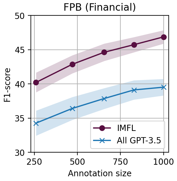

Usage
The merged.json file is a mapping between the figure's filename as stored in the repository and its caption, label, and context.
To use, you must extract the parts located under dataset/figures/ and keep the raw images in the same directory so that they match the image_filename fields.
The images are named in the format <paper id>-<figure name> where paper id is the id given by arXiv and figure name is the name of the figure as given in the raw format of each paper.
Contributors
Yousef Gomaa (@yousefg-codes) and Mohamed Awadalla (@mawadalla)
Dataset Summary
This dataset includes ~690,000 figures from ~150,000 scientific papers taken from arXiv papers. Each object in the json file is a single research paper with a list of figures each with their caption and surrounding context.
| Category | Count |
|---|---|
| Figure | 690883 |
| Paper | 152504 |
Data Instances
An example of an object in the merged.json file:
{
  [
    {
      'image_filename': 'dataset/figures/example.png' (or .eps or .pdf or other type),
      'label': 'fig_example',
      'caption': 'an example caption for this figure',
      'context': ['example context where this figure was referenced', 'up to 600 characters']
    },
  ...
  ]
}
Dataset Creation
We utilized the bulk access of arXiv's papers.
Curation Rationale
[More Information Needed]
Source Data
Initial Data Collection and Normalization
[More Information Needed]
Who are the source language producers?
[More Information Needed]
Annotations
Annotation process
[More Information Needed]
Who are the annotators?
[More Information Needed]
Personal and Sensitive Information
[More Information Needed]
Considerations for Using the Data
Social Impact of Dataset
[More Information Needed]
Discussion of Biases
[More Information Needed]
Other Known Limitations
[More Information Needed]
Additional Information
Dataset Curators
[More Information Needed]
Citation Information
coming soon
- Downloads last month
- 1