A Q-Learning example

To better understand Q-Learning, let’s take a simple example:

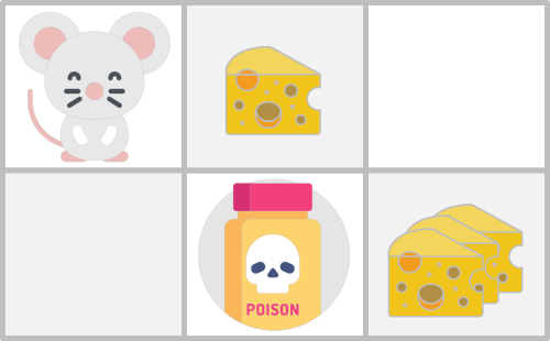
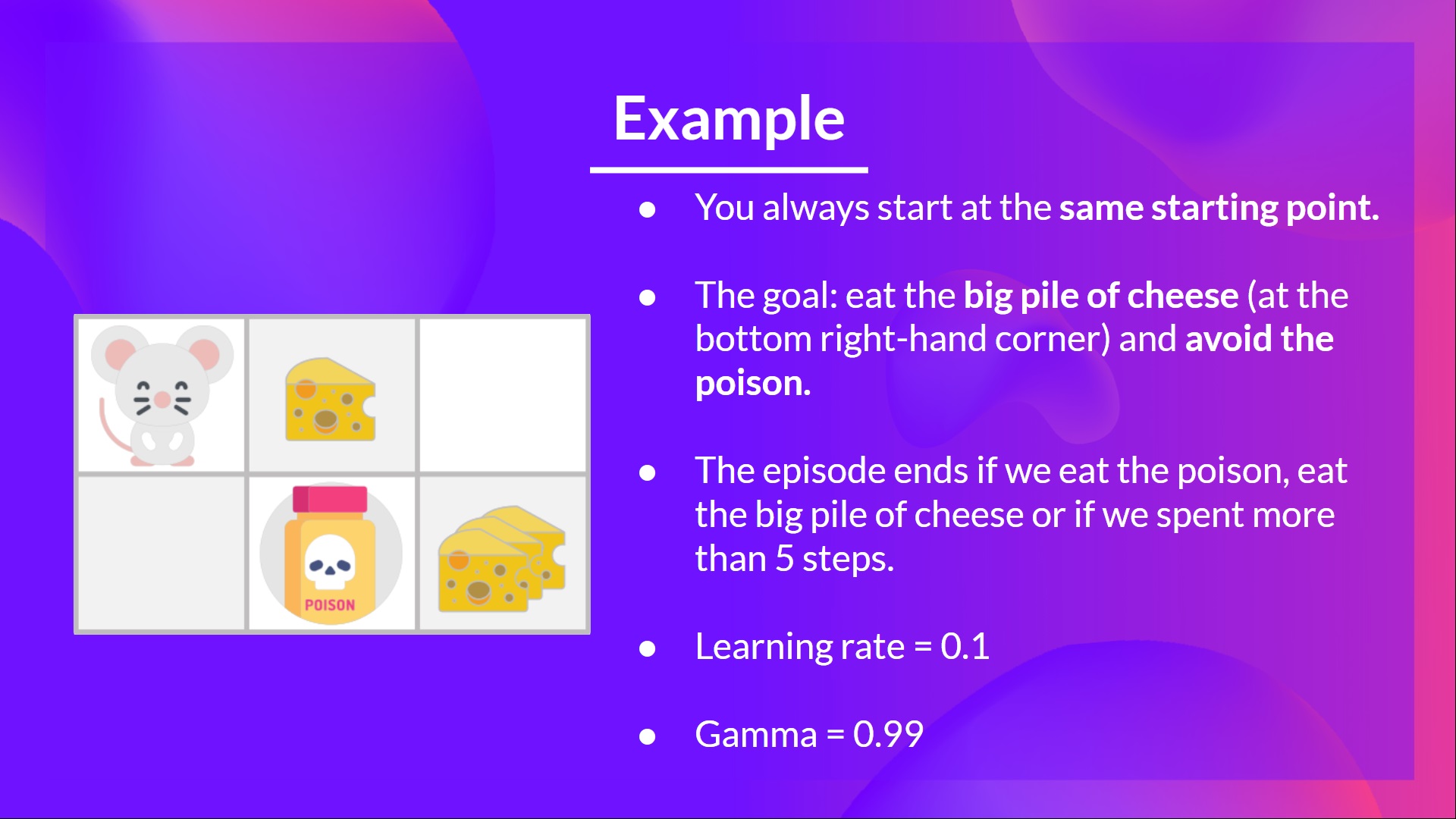
• You’re a mouse in this tiny maze. You always start at the same starting point.
• The goal is to eat the big pile of cheese at the bottom right-hand corner and avoid the poison. After all, who doesn’t like cheese?
• The episode ends if we eat the poison, eat the big pile of cheese or if we spent more than five steps.
• The learning rate is 0.1
• The gamma (discount rate) is 0.99

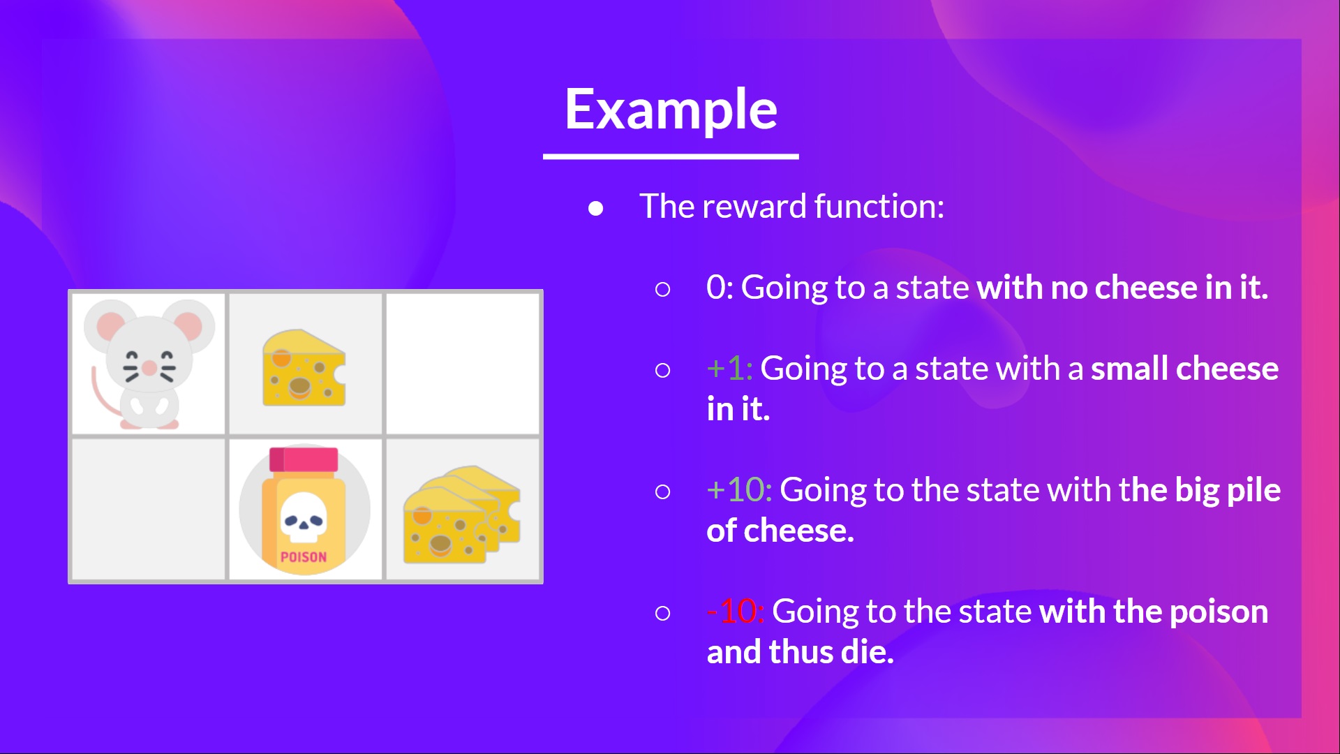
The reward function goes like this:

• +0: Going to a state with no cheese in it.
• +1: Going to a state with a small cheese in it.
• +10: Going to the state with the big pile of cheese.
• -10: Going to the state with the poison and thus die.
• +0 If we spend more than five steps.

To train our agent to have an optimal policy (so a policy that goes right, right, down), we will use the Q-Learning algorithm.

Step 1: We initialize the Q-table

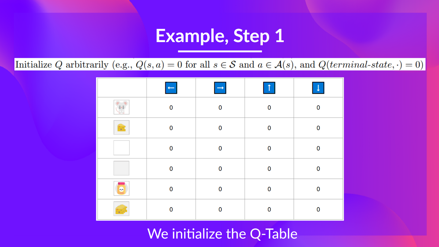
So, for now, our Q-table is useless; we need to train our Q-function using the Q-Learning algorithm.

Let’s do it for 2 training timesteps:

Training timestep 1:

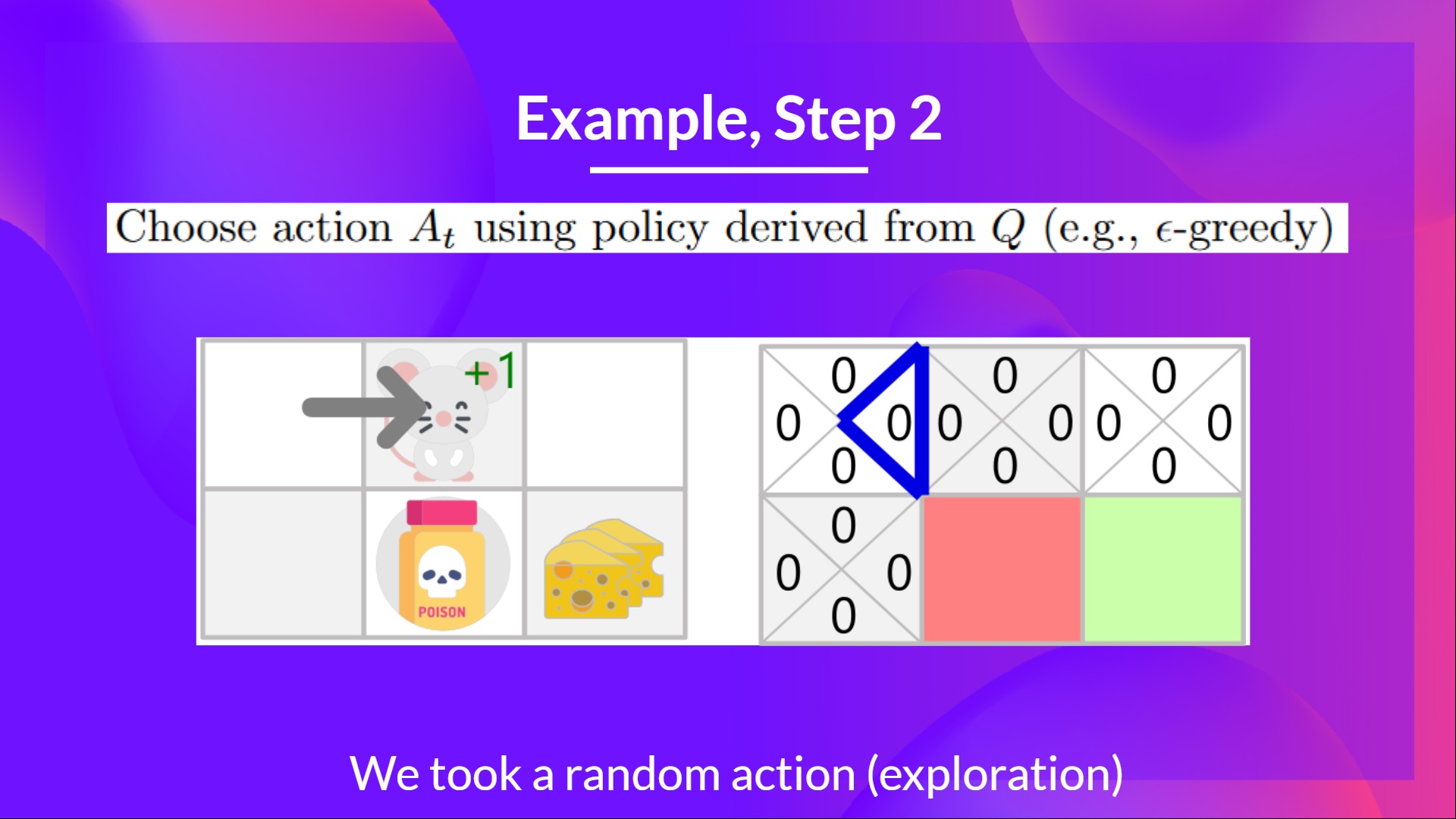
Step 2: Choose action using Epsilon Greedy Strategy

Because epsilon is big = 1.0, I take a random action, in this case, I go right.

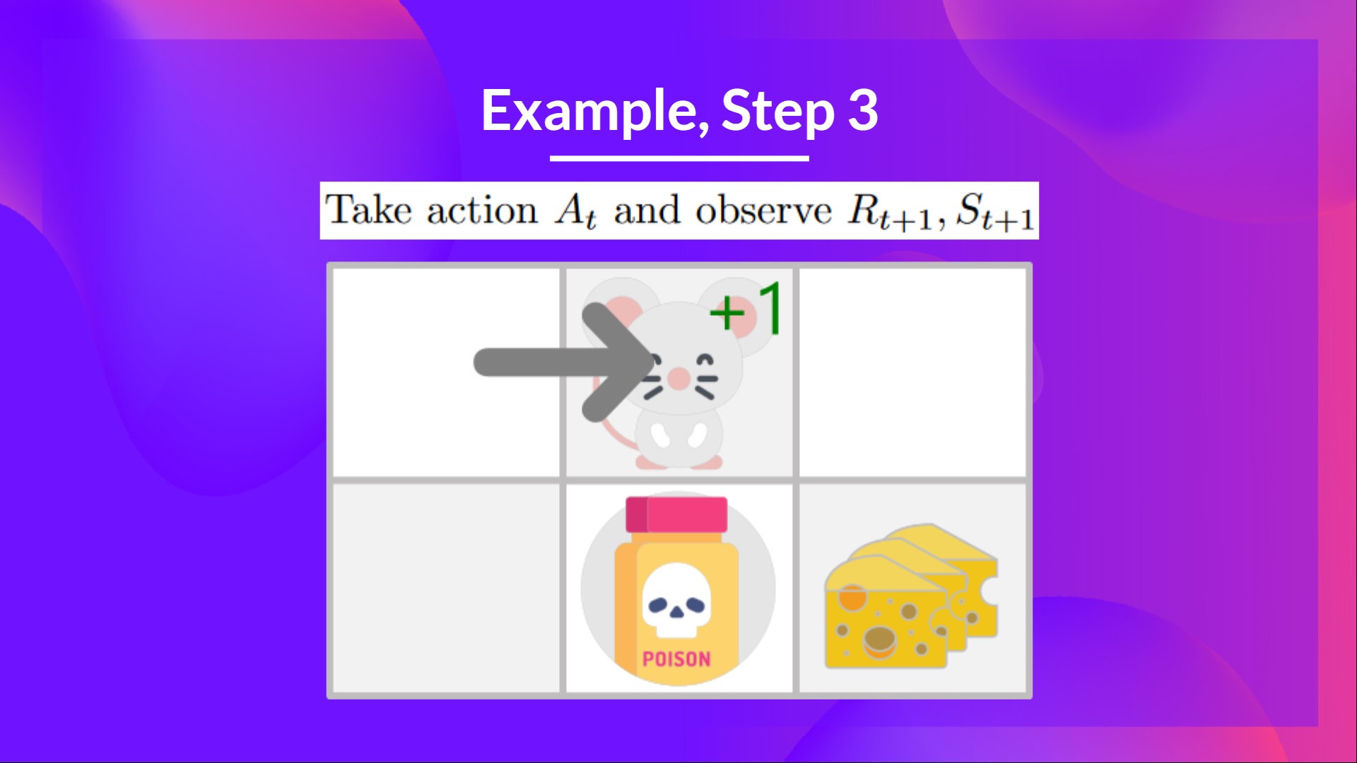
Step 3: Perform action At, gets Rt+1 and St+1

By going right, I’ve got a small cheese, so $R_{t+1} = 1$, and I’m in a new state.

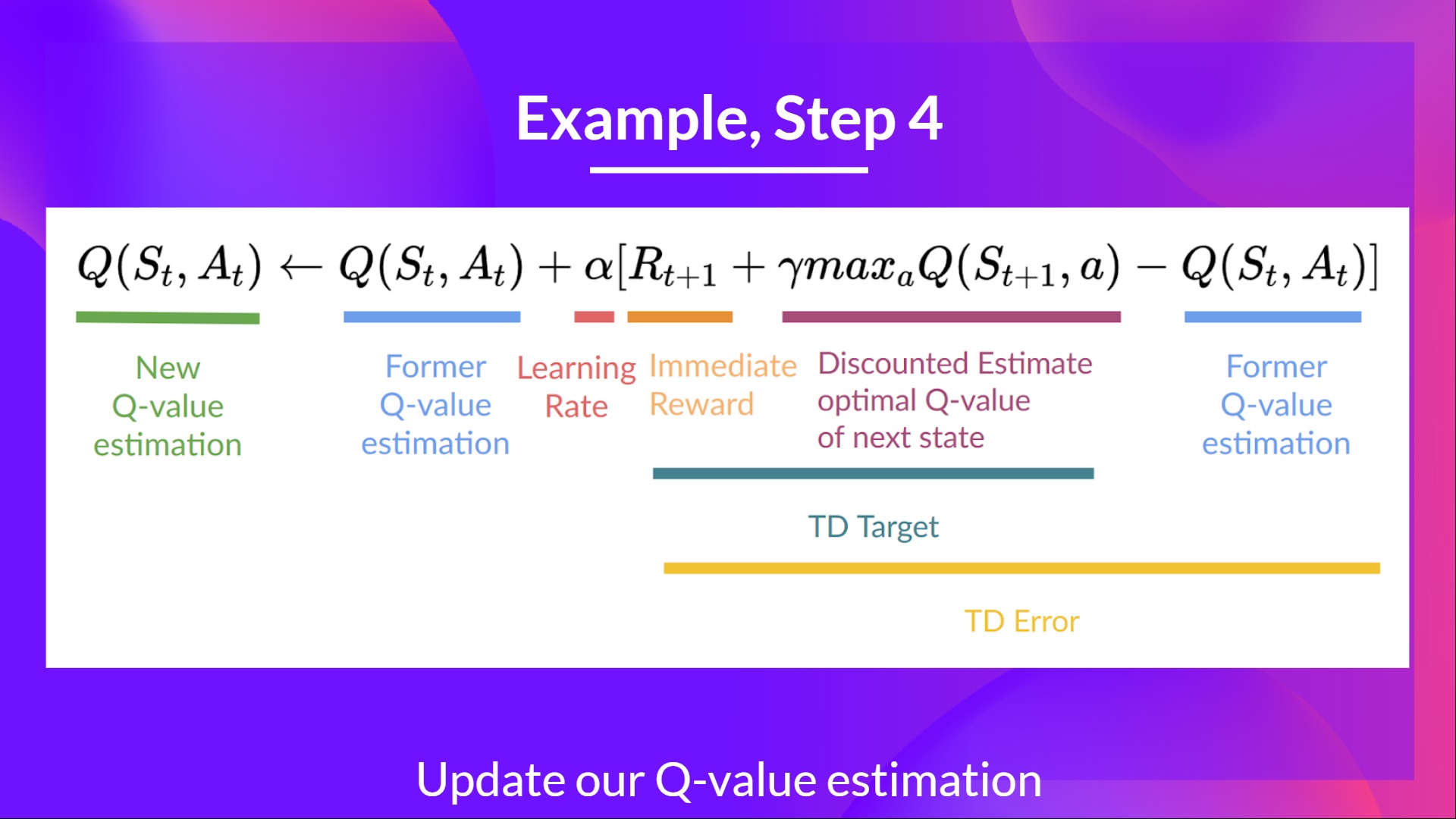
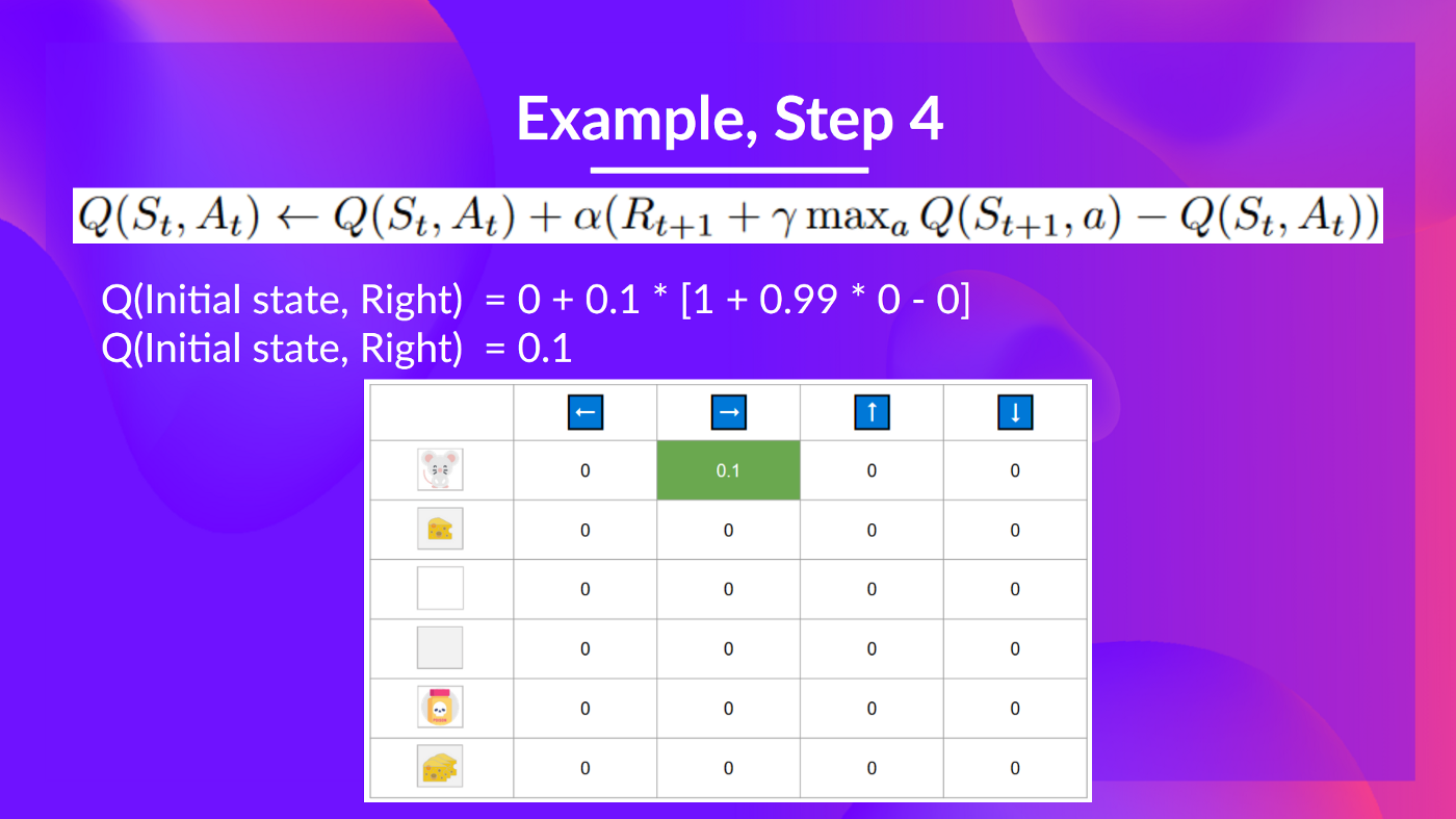
Step 4: Update Q(St, At)

We can now update $Q(S_t, A_t)$ using our formula.

Training timestep 2:

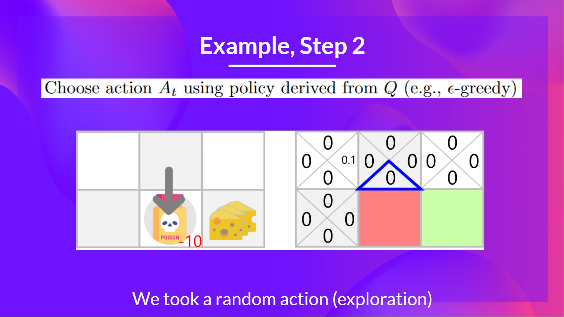
Step 2: Choose action using Epsilon Greedy Strategy

I take a random action again, since epsilon is big 0.99 (since we decay it a little bit because as the training progress, we want less and less exploration).

I took action down. Not a good action since it leads me to the poison.

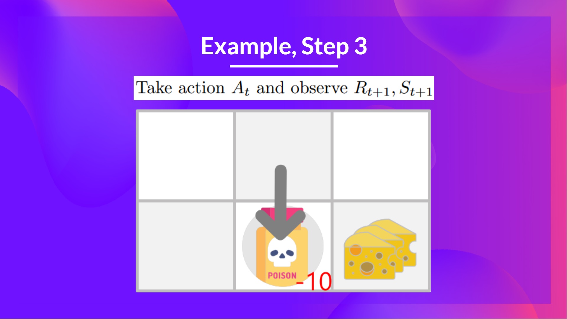
Step 3: Perform action At, gets Rt+1 and St+1

Because I go to the poison state, I get $R_{t+1} = -10$, and I die.

Step 4: Update Q(St, At)

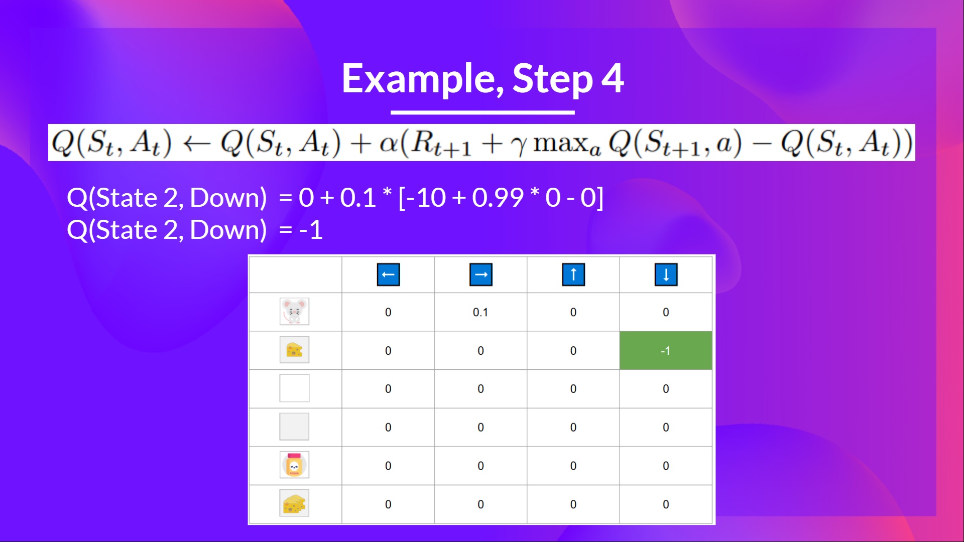
Because we’re dead, we start a new episode. But what we see here is that with two explorations steps, my agent became smarter.

As we continue exploring and exploiting the environment and updating Q-values using TD target, Q-table will give us better and better approximations. And thus, at the end of the training, we’ll get an estimate of the optimal Q-function.