[INST] {{ user_msg_2 }} [/INST] ``` This same format can be used with Code Llama Instruct to engage in technical conversations with a code-savvy assistant! Please, refer to [our Llama 2 blog post](https://huggingface.co/blog/llama2#how-to-prompt-llama-2) for more details. ### Code infilling with Code Llama Code models like Code Llama can be used for code completion using the same generation strategy we used in the previous examples: you provide a starting string that may contain code or comments, and the model will try to continue the sequence with plausible content. Code models can also be used for _infilling_, a more specialized task where you provide prefix and suffix sequences, and the model will predict what should go in between. This is great for applications such as IDE extensions. Let's see an example using Code Llama: ```Python client = InferenceClient(model=""codellama/CodeLlama-13b-hf"", token=YOUR_TOKEN) prompt_prefix = 'def remove_non_ascii(s: str) -> str:\n """""" ' prompt_suffix = ""\n return result"" prompt = f"" {prompt_prefix} {prompt_suffix} "" infilled = client.text_generation(prompt, max_new_tokens=150) infilled = infilled.rstrip("" "") print(f""{prompt_prefix}{infilled}{prompt_suffix}"") ``` ``` def remove_non_ascii(s: str) -> str: """""" Remove non-ASCII characters from a string. Args: s (str): The string to remove non-ASCII characters from. Returns: str: The string with non-ASCII characters removed. """""" result = """" for c in s: if ord(c) < 128: result += c return result ``` As you can see, the format used for infilling follows this pattern: ``` prompt = f"" {prompt_prefix} {prompt_suffix} "" ``` For more details on how this task works, please take a look at https://huggingface.co/blog/codellama#code-completion. ### Stable Diffusion XL SDXL is also available for PRO users. The response returned by the endpoint consists of a byte stream representing the generated image. If you use `InferenceClient`, it will automatically decode to a `PIL` image for you: ```Python sdxl = InferenceClient(model=""stabilityai/stable-diffusion-xl-base-1.0"", token=YOUR_TOKEN) image = sdxl.text_to_image( ""Dark gothic city in a misty night, lit by street lamps. A man in a cape is walking away from us"", guidance_scale=9, ) ```  For more details on how to control generation, please take a look at [this section](#controlling-image-generation). ## Generation Parameters ### Controlling Text Generation Text generation is a rich topic, and there exist several generation strategies for different purposes. We recommend [this excellent overview](https://huggingface.co/blog/how-to-generate) on the subject. Many generation algorithms are supported by the text generation endpoints, and they can be configured using the following parameters: - `do_sample`: If set to `False` (the default), the generation method will be _greedy search_, which selects the most probable continuation sequence after the prompt you provide. Greedy search is deterministic, so the same results will always be returned from the same input. When `do_sample` is `True`, tokens will be sampled from a probability distribution and will therefore vary across invocations. - `temperature`: Controls the amount of variation we desire from the generation. A temperature of `0` is equivalent to greedy search. If we set a value for `temperature`, then `do_sample` will automatically be enabled. The same thing happens for `top_k` and `top_p`. When doing code-related tasks, we want less variability and hence recommend a low `temperature`. For other tasks, such as open-ended text generation, we recommend a higher one. - `top_k`. Enables ""Top-K"" sampling: the model will choose from the `K` most probable tokens that may occur after the input sequence. Typical values are between 10 to 50. - `top_p`. Enables ""nucleus sampling"": the model will choose from as many tokens as necessary to cover a particular probability mass. If `top_p` is 0.9, the 90% most probable tokens will be considered for sampling, and the trailing 10% will be ignored. - `repetition_penalty`: Tries to avoid repeated words in the generated sequence. - `seed`: Random seed that you can use in combination with sampling, for reproducibility purposes. In addition to the sampling parameters above, you can also control general aspects of the generation with the following: - `max_new_tokens`: maximum number of new tokens to generate. The default is `20`, feel free to increase if you want longer sequences. - `return_full_text`: whether to include the input sequence in the output returned by the endpoint. The default used by `InferenceClient` is `False`, but the endpoint itself uses `True` by default. - `stop_sequences`: a list of sequences that will cause generation to stop when encountered in the output. ### Controlling Image Generation If you want finer-grained control over images generated with the SDXL endpoint, you can use the following parameters: - `negative_prompt`: A text describing content that you want the model to steer _away_ from. - `guidance_scale`: How closely you want the model to match the prompt. Lower numbers are less accurate, very high numbers might decrease image quality or generate artifacts. - `width` and `height`: The desired image dimensions. SDXL works best for sizes between 768 and 1024. - `num_inference_steps`: The number of denoising steps to run. Larger numbers may produce better quality but will be slower. Typical values are between 20 and 50 steps. For additional details on text-to-image generation, we recommend you check the [diffusers library documentation](https://huggingface.co/docs/diffusers/using-diffusers/sdxl). ### Caching If you run the same generation multiple times, you’ll see that the result returned by the API is the same (even if you are using sampling instead of greedy decoding). This is because recent results are cached. To force a different response each time, we can use an HTTP header to tell the server to run a new generation each time: `x-use-cache: 0`. If you are using `InferenceClient`, you can simply append it to the `headers` client property: ```Python client = InferenceClient(model=""meta-llama/Llama-2-70b-chat-hf"", token=YOUR_TOKEN) client.headers[""x-use-cache""] = ""0"" output = client.text_generation(""In a surprising turn of events, "", do_sample=True) print(output) ``` ### Streaming Token streaming is the mode in which the server returns the tokens one by one as the model generates them. This enables showing progressive generations to the user rather than waiting for the whole generation. Streaming is an essential aspect of the end-user experience as it reduces latency, one of the most critical aspects of a smooth experience. ![]()
![]()
To stream tokens with `InferenceClient`, simply pass `stream=True` and iterate over the response. ```python for token in client.text_generation(""How do you make cheese?"", max_new_tokens=12, stream=True): print(token) # To # make # cheese #, # you # need # to # start # with # milk ``` To use the generate_stream endpoint with curl, you can add the `-N`/`--no-buffer` flag, which disables curl default buffering and shows data as it arrives from the server. ``` curl -N https://api-inference.huggingface.co/models/meta-llama/Llama-2-70b-chat-hf \ -X POST \ -d '{""inputs"": ""In a surprising turn of events, "", ""parameters"": {""temperature"": 0.7, ""max_new_tokens"": 100}}' \ -H ""Content-Type: application/json"" \ -H ""Authorization: Bearer "" ``` ## Subscribe to PRO You can sign up today for a PRO subscription [here](https://huggingface.co/subscribe/pro). Benefit from higher rate limits, custom accelerated endpoints for the latest models, and early access to features. If you've built some exciting projects with the Inference API or are looking for a model not available in Inference for PROs, please [use this discussion](https://huggingface.co/spaces/huggingface/HuggingDiscussions/discussions/13). [Enterprise users](https://huggingface.co/enterprise) also benefit from PRO Inference API on top of other features, such as SSO. ## FAQ **Does this affect the free Inference API?** No. We still expose thousands of models through free APIs that allow people to prototype and explore model capabilities quickly. **Does this affect Enterprise users?** Users with an Enterprise subscription also benefit from accelerated inference API for curated models. **Can I use my own models with PRO Inference API?** The free Inference API already supports a wide range of small and medium models from a variety of libraries (such as diffusers, transformers, and sentence transformers). If you have a custom model or custom inference logic, we recommend using [Inference Endpoints](https://ui.endpoints.huggingface.co/catalog)."
Llama 2 on Amazon SageMaker a Benchmark,philschmid,"September 26, 2023",llama-sagemaker-benchmark,"guide, inference, llm, aws",https://huggingface.co/blog/llama-sagemaker-benchmark," # Llama 2 on Amazon SageMaker a Benchmark  Deploying large language models (LLMs) and other generative AI models can be challenging due to their computational requirements and latency needs. To provide useful recommendations to companies looking to deploy Llama 2 on Amazon SageMaker with the [Hugging Face LLM Inference Container](https://huggingface.co/blog/sagemaker-huggingface-llm), we created a comprehensive benchmark analyzing over 60 different deployment configurations for Llama 2. In this benchmark, we evaluated varying sizes of Llama 2 on a range of Amazon EC2 instance types with different load levels. Our goal was to measure latency (ms per token), and throughput (tokens per second) to find the optimal deployment strategies for three common use cases: - Most Cost-Effective Deployment: For users looking for good performance at low cost - Best Latency Deployment: Minimizing latency for real-time services - Best Throughput Deployment: Maximizing tokens processed per second To keep this benchmark fair, transparent, and reproducible, we share all of the assets, code, and data we used and collected: - [GitHub Repository](https://github.com/philschmid/text-generation-inference-tests/tree/master/sagemaker_llm_container) - [Raw Data](https://github.com/philschmid/text-generation-inference-tests/tree/master/results/sagemaker) - [Spreadsheet with processed data](https://docs.google.com/spreadsheets/d/1PBjw6aG3gPaoxd53vp7ZtCdPngExi2vWPC0kPZXaKlw/edit?usp=sharing) We hope to enable customers to use LLMs and Llama 2 efficiently and optimally for their use case. Before we get into the benchmark and data, let's look at the technologies and methods we used. - [Llama 2 on Amazon SageMaker a Benchmark](#llama-2-on-amazon-sagemaker-a-benchmark) - [What is the Hugging Face LLM Inference Container?](#what-is-the-hugging-face-llm-inference-container) - [What is Llama 2?](#what-is-llama-2) - [What is GPTQ?](#what-is-gptq) - [Benchmark](#benchmark) - [Recommendations \& Insights](#recommendations--insights) - [Most Cost-Effective Deployment](#most-cost-effective-deployment) - [Best Throughput Deployment](#best-throughput-deployment) - [Best Latency Deployment](#best-latency-deployment) - [Conclusions](#conclusions) ### What is the Hugging Face LLM Inference Container? [Hugging Face LLM DLC](https://huggingface.co/blog/sagemaker-huggingface-llm) is a purpose-built Inference Container to easily deploy LLMs in a secure and managed environment. The DLC is powered by [Text Generation Inference (TGI)](https://github.com/huggingface/text-generation-inference), an open-source, purpose-built solution for deploying and serving LLMs. TGI enables high-performance text generation using Tensor Parallelism and dynamic batching for the most popular open-source LLMs, including StarCoder, BLOOM, GPT-NeoX, Falcon, Llama, and T5. VMware, IBM, Grammarly, Open-Assistant, Uber, Scale AI, and many more already use Text Generation Inference. ### What is Llama 2? Llama 2 is a family of LLMs from Meta, trained on 2 trillion tokens. Llama 2 comes in three sizes - 7B, 13B, and 70B parameters - and introduces key improvements like longer context length, commercial licensing, and optimized chat abilities through reinforcement learning compared to Llama (1). If you want to learn more about Llama 2 check out this [blog post](https://huggingface.co/blog/llama2). ### What is GPTQ? GPTQ is a post-training quantziation method to compress LLMs, like GPT. GPTQ compresses GPT (decoder) models by reducing the number of bits needed to store each weight in the model, from 32 bits down to just 3-4 bits. This means the model takes up much less memory and can run on less Hardware, e.g. Single GPU for 13B Llama2 models. GPTQ analyzes each layer of the model separately and approximates the weights to preserve the overall accuracy. If you want to learn more and how to use it, check out [Optimize open LLMs using GPTQ and Hugging Face Optimum](https://www.philschmid.de/gptq-llama). ## Benchmark To benchmark the real-world performance of Llama 2, we tested 3 model sizes (7B, 13B, 70B parameters) on four different instance types with four different load levels, resulting in 60 different configurations: - Models: We evaluated all currently available model sizes, including 7B, 13B, and 70B. - Concurrent Requests: We tested configurations with 1, 5, 10, and 20 concurrent requests to determine the performance on different usage scenarios. - Instance Types: We evaluated different GPU instances, including g5.2xlarge, g5.12xlarge, g5.48xlarge powered by NVIDIA A10G GPUs, and p4d.24xlarge powered by NVIDIA A100 40GB GPU. - Quantization: We compared performance with and without quantization. We used GPTQ 4-bit as a quantization technique. As metrics, we used Throughput and Latency defined as: - Throughput (tokens/sec): Number of tokens being generated per second. - Latency (ms/token): Time it takes to generate a single token We used those to evaluate the performance of Llama across the different setups to understand the benefits and tradeoffs. If you want to run the benchmark yourself, we created a [Github repository](https://github.com/philschmid/text-generation-inference-tests/tree/master/sagemaker_llm_container). You can find the full data of the benchmark in the [Amazon SageMaker Benchmark: TGI 1.0.3 Llama 2](https://docs.google.com/spreadsheets/d/1PBjw6aG3gPaoxd53vp7ZtCdPngExi2vWPC0kPZXaKlw/edit#gid=0) sheet. The raw data is available on [GitHub](https://github.com/philschmid/text-generation-inference-tests/tree/master/results/sagemaker). If you are interested in all of the details, we recommend you to dive deep into the provided raw data. ## Recommendations & Insights Based on the benchmark, we provide specific recommendations for optimal LLM deployment depending on your priorities between cost, throughput, and latency for all Llama 2 model sizes. *Note: The recommendations are based on the configuration we tested. In the future, other environments or hardware offerings, such as Inferentia2, may be even more cost-efficient.* ### Most Cost-Effective Deployment The most cost-effective configuration focuses on the right balance between performance (latency and throughput) and cost. Maximizing the output per dollar spent is the goal. We looked at the performance during 5 concurrent requests. We can see that GPTQ offers the best cost-effectiveness, allowing customers to deploy Llama 2 13B on a single GPU. | Model | Quantization | Instance | concurrent requests | Latency (ms/token) median | Throughput (tokens/second) | On-demand cost ($/h) in us-west-2 | Time to generate 1 M tokens (minutes) | cost to generate 1M tokens ($) | | ----------- | ------------ | -------------- | ------------------- | ------------------------- | -------------------------- | --------------------------------- | ------------------------------------- | ------------------------------ | | Llama 2 7B | GPTQ | g5.2xlarge | 5 | 34.245736 | 120.0941633 | $1.52 | 138.78 | $3.50 | | Llama 2 13B | GPTQ | g5.2xlarge | 5 | 56.237484 | 71.70560104 | $1.52 | 232.43 | $5.87 | | Llama 2 70B | GPTQ | ml.g5.12xlarge | 5 | 138.347928 | 33.33372399 | $7.09 | 499.99 | $59.08 | ### Best Throughput Deployment The Best Throughput configuration maximizes the number of tokens that are generated per second. This might come with some reduction in overall latency since you process more tokens simultaneously. We looked at the highest tokens per second performance during twenty concurrent requests, with some respect to the cost of the instance. The highest throughput was for Llama 2 13B on the ml.p4d.24xlarge instance with 688 tokens/sec. | Model | Quantization | Instance | concurrent requests | Latency (ms/token) median | Throughput (tokens/second) | On-demand cost ($/h) in us-west-2 | Time to generate 1 M tokens (minutes) | cost to generate 1M tokens ($) | | ----------- | ------------ | --------------- | ------------------- | ------------------------- | -------------------------- | --------------------------------- | ------------------------------------- | ------------------------------ | | Llama 2 7B | None | ml.g5.12xlarge | 20 | 43.99524 | 449.9423027 | $7.09 | 33.59 | $3.97 | | Llama 2 13B | None | ml.p4d.12xlarge | 20 | 67.4027465 | 668.0204881 | $37.69 | 24.95 | $15.67 | | Llama 2 70B | None | ml.p4d.24xlarge | 20 | 59.798591 | 321.5369158 | $37.69 | 51.83 | $32.56 | ### Best Latency Deployment The Best Latency configuration minimizes the time it takes to generate one token. Low latency is important for real-time use cases and providing a good experience to the customer, e.g. Chat applications. We looked at the lowest median for milliseconds per token during 1 concurrent request. The lowest overall latency was for Llama 2 7B on the ml.g5.12xlarge instance with 16.8ms/token. | Model | Quantization | Instance | concurrent requests | Latency (ms/token) median | Thorughput (tokens/second) | On-demand cost ($/h) in us-west-2 | Time to generate 1 M tokens (minutes) | cost to generate 1M tokens ($) | | ----------- | ------------ | --------------- | ------------------- | ------------------------- | -------------------------- | --------------------------------- | ------------------------------------- | ------------------------------ | | Llama 2 7B | None | ml.g5.12xlarge | 1 | 16.812526 | 61.45733054 | $7.09 | 271.19 | $32.05 | | Llama 2 13B | None | ml.g5.12xlarge | 1 | 21.002715 | 47.15736567 | $7.09 | 353.43 | $41.76 | | Llama 2 70B | None | ml.p4d.24xlarge | 1 | 41.348543 | 24.5142928 | $37.69 | 679.88 | $427.05 | ## Conclusions In this benchmark, we tested 60 configurations of Llama 2 on Amazon SageMaker. For cost-effective deployments, we found 13B Llama 2 with GPTQ on g5.2xlarge delivers 71 tokens/sec at an hourly cost of $1.55. For max throughput, 13B Llama 2 reached 296 tokens/sec on ml.g5.12xlarge at $2.21 per 1M tokens. And for minimum latency, 7B Llama 2 achieved 16ms per token on ml.g5.12xlarge. We hope the benchmark will help companies deploy Llama 2 optimally based on their needs. If you want to get started deploying Llama 2 on Amazon SageMaker, check out [Introducing the Hugging Face LLM Inference Container for Amazon SageMaker](https://huggingface.co/blog/sagemaker-huggingface-llm) and [Deploy Llama 2 7B/13B/70B on Amazon SageMaker](https://www.philschmid.de/sagemaker-llama-llm) blog posts. --- Thanks for reading! If you have any questions, feel free to contact me on [Twitter](https://twitter.com/_philschmid) or [LinkedIn](https://www.linkedin.com/in/philipp-schmid-a6a2bb196/)."
Non-engineers guide: Train a LLaMA 2 chatbot,2legit2overfit,"September 28, 2023",Llama2-for-non-engineers,"guide, community, nlp",https://huggingface.co/blog/Llama2-for-non-engineers," # Non-engineers guide: Train a LLaMA 2 chatbot ## Introduction In this tutorial we will show you how anyone can build their own open-source ChatGPT without ever writing a single line of code! We’ll use the LLaMA 2 base model, fine tune it for chat with an open-source instruction dataset and then deploy the model to a chat app you can share with your friends. All by just clicking our way to greatness. 😀 Why is this important? Well, machine learning, especially LLMs (Large Language Models), has witnessed an unprecedented surge in popularity, becoming a critical tool in our personal and business lives. Yet, for most outside the specialized niche of ML engineering, the intricacies of training and deploying these models appears beyond reach. If the anticipated future of machine learning is to be one filled with ubiquitous personalized models, then there's an impending challenge ahead: How do we empower those with non-technical backgrounds to harness this technology independently? At Hugging Face, we’ve been quietly working to pave the way for this inclusive future. Our suite of tools, including services like Spaces, AutoTrain, and Inference Endpoints, are designed to make the world of machine learning accessible to everyone. To showcase just how accessible this democratized future is, this tutorial will show you how to use [Spaces](https://huggingface.co/Spaces), [AutoTrain](https://huggingface.co/autotrain) and [ChatUI](https://huggingface.co/inference-endpoints) to build the chat app. All in just three simple steps, sans a single line of code. For context I’m also not an ML engineer, but a member of the Hugging Face GTM team. If I can do this then you can too! Let's dive in! ## Introduction to Spaces Spaces from Hugging Face is a service that provides easy to use GUI for building and deploying web hosted ML demos and apps. The service allows you to quickly build ML demos using Gradio or Streamlit front ends, upload your own apps in a docker container, or even select a number of pre-configured ML applications to deploy instantly. We’ll be deploying two of the pre-configured docker application templates from Spaces, AutoTrain and ChatUI. You can read more about Spaces [here](https://huggingface.co/docs/hub/spaces). ## Introduction to AutoTrain AutoTrain is a no-code tool that lets non-ML Engineers, (or even non-developers 😮) train state-of-the-art ML models without the need to code. It can be used for NLP, computer vision, speech, tabular data and even now for fine-tuning LLMs like we’ll be doing today. You can read more about AutoTrain [here](https://huggingface.co/docs/autotrain/index). ## Introduction to ChatUI ChatUI is exactly what it sounds like, it’s the open-source UI built by Hugging Face that provides an interface to interact with open-source LLMs. Notably, it's the same UI behind HuggingChat, our 100% open-source alternative to ChatGPT. You can read more about ChatUI [here](https://github.com/huggingface/chat-ui). ### Step 1: Create a new AutoTrain Space 1.1 Go to [huggingface.co/spaces](https://huggingface.co/spaces) and select “Create new Space”. ![]()
1.2 Give your Space a name and select a preferred usage license if you plan to make your model or Space public. 1.3 In order to deploy the AutoTrain app from the Docker Template in your deployed space select Docker > AutoTrain. ![]()
1.4 Select your “Space hardware” for running the app. (Note: For the AutoTrain app the free CPU basic option will suffice, the model training later on will be done using separate compute which we can choose later) 1.5 Add your “HF_TOKEN” under “Space secrets” in order to give this Space access to your Hub account. Without this the Space won’t be able to train or save a new model to your account. (Note: Your HF_TOKEN can be found in your Hugging Face Profile under Settings > Access Tokens, make sure the token is selected as “Write”) 1.6 Select whether you want to make the “Private” or “Public”, for the AutoTrain Space itself it’s recommended to keep this Private, but you can always publicly share your model or Chat App later on. 1.7 Hit “Create Space” et voilà! The new Space will take a couple of minutes to build after which you can open the Space and start using AutoTrain. ![]()
### Step 2: Launch a Model Training in AutoTrain 2.1 Once you’re AutoTrain space has launched you’ll see the GUI below. AutoTrain can be used for several different kinds of training including LLM fine-tuning, text classification, tabular data and diffusion models. As we’re focusing on LLM training today select the “LLM” tab. 2.2 Choose the LLM you want to train from the “Model Choice” field, you can select a model from the list or type the name of the model from the Hugging Face model card, in this example we’ve used Meta’s Llama 2 7b foundation model, learn more from the model card [here](https://huggingface.co/meta-llama/Llama-2-7b-hf). (Note: LLama 2 is gated model which requires you to request access from Meta before using, but there are plenty of others non-gated models you could choose like Falcon) 2.3 In “Backend” select the CPU or GPU you want to use for your training. For a 7b model an “A10G Large” will be big enough. If you choose to train a larger model you’ll need to make sure the model can fully fit in the memory of your selected GPU. (Note: If you want to train a larger model and need access to an A100 GPU please email api-enterprise@huggingface.co) 2.4 Of course to fine-tune a model you’ll need to upload “Training Data”. When you do, make sure the dataset is correctly formatted and in CSV file format. An example of the required format can be found [here](https://huggingface.co/docs/autotrain/main/en/llm_finetuning). If your dataset contains multiple columns, be sure to select the “Text Column” from your file that contains the training data. In this example we’ll be using the Alpaca instruction tuning dataset, more information about this dataset is available [here](https://huggingface.co/datasets/tatsu-lab/alpaca). You can also download it directly as CSV from [here](https://huggingface.co/datasets/tofighi/LLM/resolve/main/alpaca.csv). ![]()
2.5 Optional: You can upload “Validation Data” to test your newly trained model against, but this isn’t required. 2.6 A number of advanced settings can be configured in AutoTrain to reduce the memory footprint of your model like changing precision (“FP16”), quantization (“Int4/8”) or whether to employ PEFT (Parameter Efficient Fine Tuning). It’s recommended to use these as is set by default as it will reduce the time and cost to train your model, and only has a small impact on model performance. 2.7 Similarly you can configure the training parameters in “Parameter Choice” but for now let’s use the default settings. ![]()
2.8 Now everything is set up, select “Add Job” to add the model to your training queue then select “Start Training” (Note: If you want to train multiple models versions with different hyper-parameters you can add multiple jobs to run simultaneously) 2.9 After training has started you’ll see that a new “Space” has been created in your Hub account. This Space is running the model training, once it’s complete the new model will also be shown in your Hub account under “Models”. (Note: To view training progress you can view live logs in the Space) 2.10 Go grab a coffee, depending on the size of your model and training data this could take a few hours or even days. Once completed a new model will appear in your Hugging Face Hub account under “Models”. ![]()
### Step 3: Create a new ChatUI Space using your model 3.1 Follow the same process of setting up a new Space as in steps 1.1 > 1.3, but select the ChatUI docker template instead of AutoTrain. 3.2 Select your “Space Hardware” for our 7b model an A10G Small will be sufficient to run the model, but this will vary depending on the size of your model. ![]()
3.3 If you have your own Mongo DB you can provide those details in order to store chat logs under “MONGODB_URL”. Otherwise leave the field blank and a local DB will be created automatically. 3.4 In order to run the chat app using the model you’ve trained you’ll need to provide the “MODEL_NAME” under the “Space variables” section. You can find the name of your model by looking in the “Models” section of your Hugging Face profile, it will be the same as the “Project name” you used in AutoTrain. In our example it’s “2legit2overfit/wrdt-pco6-31a7-0”. 3.4 Under “Space variables” you can also change model inference parameters including temperature, top-p, max tokens generated and others to change the nature of your generations. For now let’s stick with the default settings. ![]()
3.5 Now you are ready to hit “Create” and launch your very own open-source ChatGPT. Congratulations! If you’ve done it right it should look like this. ![]()
_If you’re feeling inspired, but still need technical support to get started, feel free to reach out and apply for support [here](https://huggingface.co/support#form). Hugging Face offers a paid Expert Advice service that might be able to help._"
Finetune Stable Diffusion Models with DDPO via TRL,metric-space,"September 29, 2023",trl-ddpo,"guide, diffusers, rl, rlhf",https://huggingface.co/blog/trl-ddpo," # Finetune Stable Diffusion Models with DDPO via TRL ## Introduction Diffusion models (e.g., DALL-E 2, Stable Diffusion) are a class of generative models that are widely successful at generating images most notably of the photorealistic kind. However, the images generated by these models may not always be on par with human preference or human intention. Thus arises the alignment problem i.e. how does one go about making sure that the outputs of a model are aligned with human preferences like “quality” or that outputs are aligned with intent that is hard to express via prompts? This is where Reinforcement Learning comes into the picture. In the world of Large Language Models (LLMs), Reinforcement learning (RL) has proven to become a very effective tool for aligning said models to human preferences. It’s one of the main recipes behind the superior performance of systems like ChatGPT. More precisely, RL is the critical ingredient of Reinforcement Learning from Human Feedback (RLHF), which makes ChatGPT chat like human beings. In [Training Diffusion Models with Reinforcement Learning, Black](https://arxiv.org/abs/2305.13301) et al. show how to augment diffusion models to leverage RL to fine-tune them with respect to an objective function via a method named Denoising Diffusion Policy Optimization (DDPO). In this blog post, we discuss how DDPO came to be, a brief description of how it works, and how DDPO can be incorporated into an RLHF workflow to achieve model outputs more aligned with the human aesthetics. We then quickly switch gears to talk about how you can apply DDPO to your models with the newly integrated `DDPOTrainer` from the `trl` library and discuss our findings from running DDPO on Stable Diffusion. ## The Advantages of DDPO DDPO is not the only working answer to the question of how to attempt to fine-tune diffusion models with RL. Before diving in, there are two key points to remember when it comes to understanding the advantages of one RL solution over the other 1. Computational efficiency is key. The more complicated your data distribution gets, the higher your computational costs get. 2. Approximations are nice, but because approximations are not the real thing, associated errors stack up. Before DDPO, Reward-weighted regression (RWR) was an established way of using Reinforcement Learning to fine-tune diffusion models. RWR reuses the denoising loss function of the diffusion model along with training data sampled from the model itself and per-sample loss weighting that depends on the reward associated with the final samples. This algorithm ignores the intermediate denoising steps/samples. While this works, two things should be noted: 1. Optimizing by weighing the associated loss, which is a maximum likelihood objective, is an approximate optimization 2. The associated loss is not an exact maximum likelihood objective but an approximation that is derived from a reweighed variational bound The two orders of approximation have a significant impact on both performance and the ability to handle complex objectives. DDPO uses this method as a starting point. Rather than viewing the denoising step as a single step by only focusing on the final sample, DDPO frames the whole denoising process as a multistep Markov Decision Process (MDP) where the reward is received at the very end. This formulation in addition to using a fixed sampler paves the way for the agent policy to become an isotropic Gaussian as opposed to an arbitrarily complicated distribution. So instead of using the approximate likelihood of the final sample (which is the path RWR takes), here the exact likelihood of each denoising step which is extremely easy to compute ( \\( \ell(\mu, \sigma^2; x) = -\frac{n}{2} \log(2\pi) - \frac{n}{2} \log(\sigma^2) - \frac{1}{2\sigma^2} \sum_{i=1}^n (x_i - \mu)^2 \\) ). If you’re interested in learning more details about DDPO, we encourage you to check out the [original paper](https://arxiv.org/abs/2305.13301) and the [accompanying blog post](https://bair.berkeley.edu/blog/2023/07/14/ddpo/). ## DDPO algorithm briefly Given the MDP framework used to model the sequential nature of the denoising process and the rest of the considerations that follow, the tool of choice to tackle the optimization problem is a policy gradient method. Specifically Proximal Policy Optimization (PPO). The whole DDPO algorithm is pretty much the same as Proximal Policy Optimization (PPO) but as a side, the portion that stands out as highly customized is the trajectory collection portion of PPO Here’s a diagram to summarize the flow: 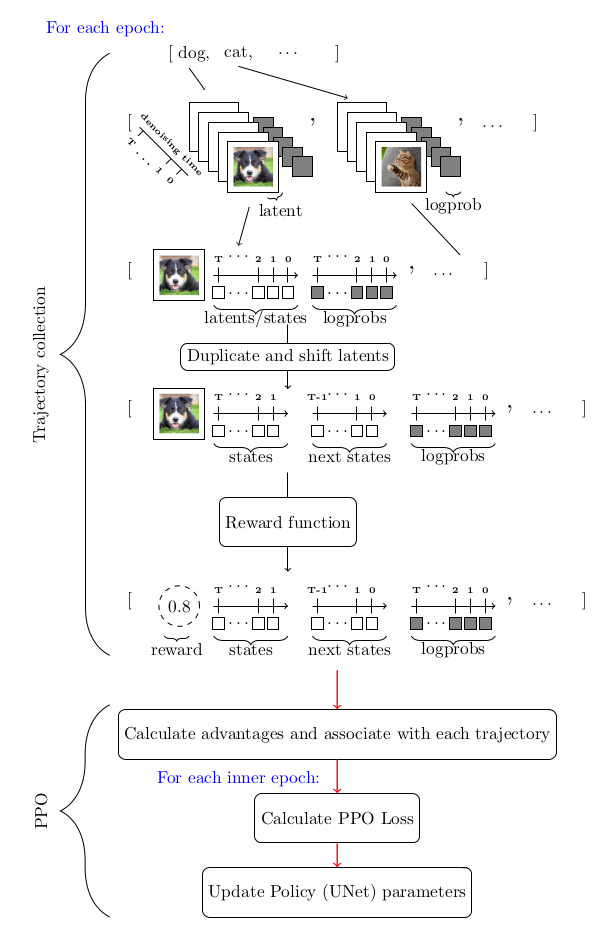 ## DDPO and RLHF: a mix to enforce aestheticness The general training aspect of [RLHF](https://huggingface.co/blog/rlhf) can roughly be broken down into the following steps: 1. Supervised fine-tuning a “base” model learns to the distribution of some new data 2. Gathering preference data and training a reward model using it. 3. Fine-tuning the model with reinforcement learning using the reward model as a signal. It should be noted that preference data is the primary source for capturing human feedback in the context of RLHF. When we add DDPO to the mix, the workflow gets morphed to the following: 1. Starting with a pretrained Diffusion Model 2. Gathering preference data and training a reward model using it. 3. Fine-tuning the model with DDPO using the reward model as a signal Notice that step 3 from the general RLHF workflow is missing in the latter list of steps and this is because empirically it has been shown (as you will get to see yourself) that this is not needed. To get on with our venture to get a diffusion model to output images more in line with the human perceived notion of what it means to be aesthetic, we follow these steps: 1. Starting with a pretrained Stable Diffusion (SD) Model 2. Training a frozen [CLIP](https://huggingface.co/openai/clip-vit-large-patch14) model with a trainable regression head on the [Aesthetic Visual Analysis](http://refbase.cvc.uab.es/files/MMP2012a.pdf) (AVA) dataset to predict how much people like an input image on average 3. Fine-tuning the SD model with DDPO using the aesthetic predictor model as the reward signaller We keep these steps in mind while moving on to actually getting these running which is described in the following sections. ## Training Stable Diffusion with DDPO ### Setup To get started, when it comes to the hardware side of things and this implementation of DDPO, at the very least access to an A100 NVIDIA GPU is required for successful training. Anything below this GPU type will soon run into Out-of-memory issues. Use pip to install the `trl` library ```bash pip install trl[diffusers] ``` This should get the main library installed. The following dependencies are for tracking and image logging. After getting `wandb` installed, be sure to login to save the results to a personal account ```bash pip install wandb torchvision ``` Note: you could choose to use `tensorboard` rather than `wandb` for which you’d want to install the `tensorboard` package via `pip`. ### A Walkthrough The main classes within the `trl` library responsible for DDPO training are the `DDPOTrainer` and `DDPOConfig` classes. See [docs](https://huggingface.co/docs/trl/ddpo_trainer#getting-started-with-examplesscriptsstablediffusiontuningpy) for more general info on the `DDPOTrainer` and `DDPOConfig`. There is an [example training script](https://github.com/huggingface/trl/blob/main/examples/scripts/ddpo.py) in the `trl` repo. It uses both of these classes in tandem with default implementations of required inputs and default parameters to finetune a default pretrained Stable Diffusion Model from `RunwayML` . This example script uses `wandb` for logging and uses an aesthetic reward model whose weights are read from a public facing HuggingFace repo (so gathering data and training the aesthetic reward model is already done for you). The default prompt dataset used is a list of animal names. There is only one commandline flag argument that is required of the user to get things up and running. Additionally, the user is expected to have a [huggingface user access token](https://huggingface.co/docs/hub/security-tokens) that will be used to upload the model post finetuning to HuggingFace hub. The following bash command gets things running: ```python python stable_diffusion_tuning.py --hf_user_access_token ``` The following table contains key hyperparameters that are directly correlated with positive results: | Parameter | Description | Recommended value for single GPU training (as of now) | | --- | --- | --- | | `num_epochs` | The number of epochs to train for | 200 | | `train_batch_size` | The batch size to use for training | 3 | | `sample_batch_size` | The batch size to use for sampling | 6 | | `gradient_accumulation_steps` | The number of accelerator based gradient accumulation steps to use | 1 | | `sample_num_steps` | The number of steps to sample for | 50 | | `sample_num_batches_per_epoch` | The number of batches to sample per epoch | 4 | | `per_prompt_stat_tracking` | Whether to track stats per prompt. If false, advantages will be calculated using the mean and std of the entire batch as opposed to tracking per prompt | `True` | | `per_prompt_stat_tracking_buffer_size` | The size of the buffer to use for tracking stats per prompt | 32 | | `mixed_precision` | Mixed precision training | `True` | | `train_learning_rate` | Learning rate | 3e-4 | The provided script is merely a starting point. Feel free to adjust the hyperparameters or even overhaul the script to accommodate different objective functions. For instance, one could integrate a function that gauges JPEG compressibility or [one that evaluates visual-text alignment using a multi-modal model](https://github.com/kvablack/ddpo-pytorch/blob/main/ddpo_pytorch/rewards.py#L45), among other possibilities. ## Lessons learned 1. The results seem to generalize over a wide variety of prompts despite the minimally sized training prompts size. This has been thoroughly verified for the objective function that rewards aesthetics 2. Attempts to try to explicitly generalize at least for the aesthetic objective function by increasing the training prompt size and varying the prompts seem to slow down the convergence rate for barely noticeable learned general behavior if at all this exists 3. While LoRA is recommended and is tried and tested multiple times, the non-LoRA is something to consider, among other reasons from empirical evidence, non-Lora does seem to produce relatively more intricate images than LoRA. However, getting the right hyperparameters for a stable non-LoRA run is significantly more challenging. 4. Recommendations for the config parameters for non-Lora are: set the learning rate relatively low, something around `1e-5` should do the trick and set `mixed_precision` to `None` ## Results The following are pre-finetuned (left) and post-finetuned (right) outputs for the prompts `bear`, `heaven` and `dune` (each row is for the outputs of a single prompt): | pre-finetuned | post-finetuned | |:-------------------------:|:-------------------------:| | 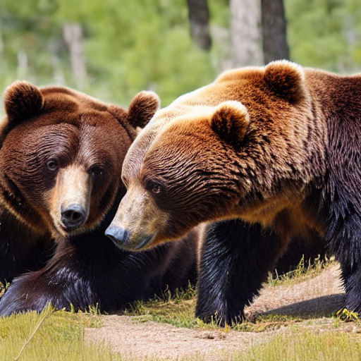 | 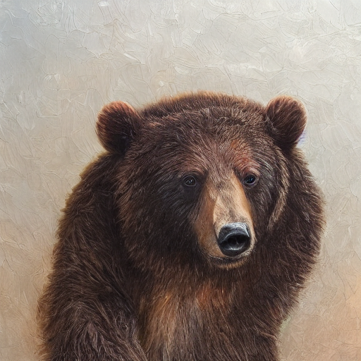 | | 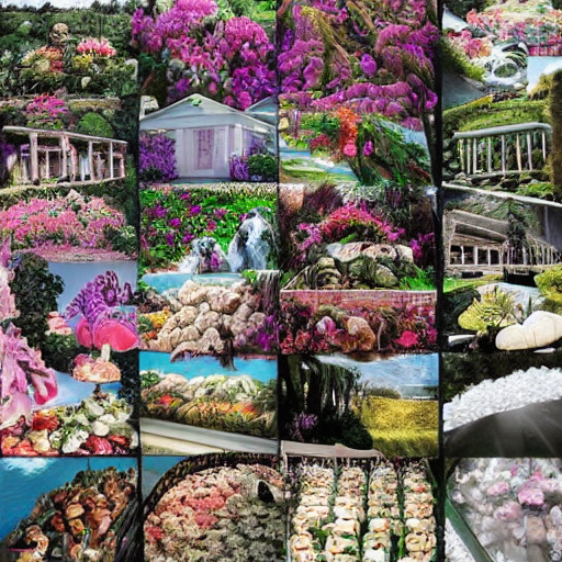 |  | |  |  | ## Limitations 1. Right now `trl`'s DDPOTrainer is limited to finetuning vanilla SD models; 2. In our experiments we primarily focused on LoRA which works very well. We did a few experiments with full training which can lead to better quality but finding the right hyperparameters is more challenging. ## Conclusion Diffusion models like Stable Diffusion, when fine-tuned using DDPO, can offer significant improvements in the quality of generated images as perceived by humans or any other metric once properly conceptualized as an objective function The computational efficiency of DDPO and its ability to optimize without relying on approximations, especially over earlier methods to achieve the same goal of fine-tuning diffusion models, make it a suitable candidate for fine-tuning diffusion models like Stable Diffusion `trl` library's `DDPOTrainer` implements DDPO for finetuning SD models. Our experimental findings underline the strength of DDPO in generalizing across a broad range of prompts, although attempts at explicit generalization through varying prompts had mixed results. The difficulty of finding the right hyperparameters for non-LoRA setups also emerged as an important learning. DDPO is a promising technique to align diffusion models with any reward function and we hope that with the release in TRL we can make it more accessible to the community! ## Acknowledgements Thanks to Chunte Lee for the thumbnail of this blog post."
Ethics and Society Newsletter #5: Hugging Face Goes To Washington and Other Summer 2023 Musings,meg,"September 29, 2023",ethics-soc-5,ethics,https://huggingface.co/blog/ethics-soc-5," # Ethics and Society Newsletter #5: Hugging Face Goes To Washington and Other Summer 2023 Musings One of the most important things to know about “ethics” in AI is that it has to do with **values**. Ethics doesn’t tell you what’s right or wrong, it provides a vocabulary of values – transparency, safety, justice – and frameworks to prioritize among them. This summer, we were able to take our understanding of values in AI to legislators in the E.U., U.K., and U.S., to help shape the future of AI regulation. This is where ethics shines: helping carve out a path forward when laws are not yet in place. In keeping with Hugging Face’s core values of *openness* and *accountability*, we are sharing a collection of what we’ve said and done here. This includes our CEO [Clem](https://huggingface.co/clem)’s [testimony to U.S. Congress](https://twitter.com/ClementDelangue/status/1673348676478025730) and [statements at the U.S. Senate AI Insight Forum](https://twitter.com/ClementDelangue/status/1702095553503412732); our advice on the [E.U. AI Act](https://huggingface.co/blog/eu-ai-act-oss); our [comments to the NTIA on AI Accountability](https://huggingface.co/blog/policy-ntia-rfc); and our Chief Ethics Scientist [Meg](https://huggingface.co/meg)’s [comments to the Democratic Caucus](assets/164_ethics-soc-5/meg_dem_caucus.pdf). Common to many of these discussions were questions about why openness in AI can be beneficial, and we share a collection of our answers to this question [here](assets/164_ethics-soc-5/why_open.md). In keeping with our core value of *democratization*, we have also spent a lot of time speaking publicly, and have been privileged to speak with journalists in order to help explain what’s happening in the world of AI right now. This includes: - Comments from [Sasha](https://huggingface.co/sasha) on **AI’s energy use and carbon emissions** ([The Atlantic](https://www.theatlantic.com/technology/archive/2023/08/ai-carbon-emissions-data-centers/675094/), [The Guardian](https://www.theguardian.com/technology/2023/aug/01/techscape-environment-cost-ai-artificial-intelligence), ([twice](https://www.theguardian.com/technology/2023/jun/08/artificial-intelligence-industry-boom-environment-toll)), [New Scientist](https://www.newscientist.com/article/2381859-shifting-where-data-is-processed-for-ai-can-reduce-environmental-harm/), [The Weather Network](https://www.theweathernetwork.com/en/news/climate/causes/how-energy-intensive-are-ai-apps-like-chatgpt), the [Wall Street Journal](https://www.wsj.com/articles/artificial-intelligence-technology-energy-a3a1a8a7), ([twice](https://www.wsj.com/articles/artificial-intelligence-can-make-companies-greener-but-it-also-guzzles-energy-7c7b678))), as well as penning part of a [Wall Street Journal op-ed on the topic](https://www.wsj.com/articles/artificial-intelligence-technology-energy-a3a1a8a7); thoughts on **AI doomsday risk** ([Bloomberg](https://www.bnnbloomberg.ca/ai-doomsday-scenarios-are-gaining-traction-in-silicon-valley-1.1945116), [The Times](https://www.thetimes.co.uk/article/everything-you-need-to-know-about-ai-but-were-afraid-to-ask-g0q8sq7zv), [Futurism](https://futurism.com/the-byte/ai-expert-were-all-going-to-die), [Sky News](https://www.youtube.com/watch?v=9Auq9mYxFEE)); details on **bias in generative AI** ([Bloomberg](https://www.bloomberg.com/graphics/2023-generative-ai-bias/), [NBC](https://www.nbcnews.com/news/asian-america/tool-reducing-asian-influence-ai-generated-art-rcna89086), [Vox](https://www.vox.com/technology/23738987/racism-ai-automated-bias-discrimination-algorithm)); addressing how **marginalized workers create the data for AI** ([The Globe and Mail](https://www.theglobeandmail.com/business/article-ai-data-gig-workers/), [The Atlantic](https://www.theatlantic.com/technology/archive/2023/07/ai-chatbot-human-evaluator-feedback/674805/)); highlighting effects of **sexism in AI** ([VICE](https://www.vice.com/en/article/g5ywp7/you-know-what-to-do-boys-sexist-app-lets-men-rate-ai-generated-women)); and providing insights in MIT Technology Review on [AI text detection](https://www.technologyreview.com/2023/07/07/1075982/ai-text-detection-tools-are-really-easy-to-fool/), [open model releases](https://www.technologyreview.com/2023/07/18/1076479/metas-latest-ai-model-is-free-for-all/), and [AI transparency](https://www.technologyreview.com/2023/07/25/1076698/its-high-time-for-more-ai-transparency/). - Comments from [Nathan](https://huggingface.co/natolambert) on the state of the art on **language models and open releases** ([WIRED](https://www.wired.com/story/metas-open-source-llama-upsets-the-ai-horse-race/), [VentureBeat](https://venturebeat.com/business/todays-ai-is-not-science-its-alchemy-what-that-means-and-why-that-matters-the-ai-beat/), [Business Insider](https://www.businessinsider.com/chatgpt-openai-moat-in-ai-wars-llama2-shrinking-2023-7), [Fortune](https://fortune.com/2023/07/18/meta-llama-2-ai-open-source-700-million-mau/)). - Comments from [Meg](https://huggingface.co/meg) on **AI and misinformation** ([CNN](https://www.cnn.com/2023/07/17/tech/ai-generated-election-misinformation-social-media/index.html), [al Jazeera](https://www.youtube.com/watch?v=NuLOUzU8P0c), [the New York Times](https://www.nytimes.com/2023/07/18/magazine/wikipedia-ai-chatgpt.html)); the need for **just handling of artists’ work** in AI ([Washington Post](https://www.washingtonpost.com/technology/2023/07/16/ai-programs-training-lawsuits-fair-use/)); advancements in **generative AI** and their relationship to the greater good ([Washington Post](https://www.washingtonpost.com/technology/2023/09/20/openai-dall-e-image-generator/), [VentureBeat](https://venturebeat.com/ai/generative-ai-secret-sauce-data-scraping-under-attack/)); how **journalists can better shape the evolution of AI** with their reporting ([CJR](https://www.cjr.org/analysis/how-to-report-better-on-artificial-intelligence.php)); as well as explaining the fundamental statistical concept of **perplexity** in AI ([Ars Technica](https://arstechnica.com/information-technology/2023/07/why-ai-detectors-think-the-us-constitution-was-written-by-ai/)); and highlighting patterns of **sexism** ([Fast Company](https://www.fastcompany.com/90952272/chuck-schumer-ai-insight-forum)). - Comments from [Irene](https://huggingface.co/irenesolaiman) on understanding the **regulatory landscape of AI** ([MIT Technology Review](https://www.technologyreview.com/2023/09/11/1079244/what-to-know-congress-ai-insight-forum-meeting/), [Barron’s](https://www.barrons.com/articles/artificial-intelligence-chips-technology-stocks-roundtable-74b256fd)). - Comments from [Yacine](https://huggingface.co/yjernite) on **open source and AI legislation** ([VentureBeat](https://venturebeat.com/ai/hugging-face-github-and-more-unite-to-defend-open-source-in-eu-ai-legislation/), [TIME](https://time.com/6308604/meta-ai-access-open-source/)) as well as **copyright issues** ([VentureBeat](https://venturebeat.com/ai/potential-supreme-court-clash-looms-over-copyright-issues-in-generative-ai-training-data/)). - Comments from [Giada](https://huggingface.co/giadap) on the concepts of **AI “singularity”** ([Popular Mechanics](https://www.popularmechanics.com/technology/security/a43929371/ai-singularity-dangers/)) and **AI “sentience”** ([RFI](https://www.rfi.fr/fr/technologies/20230612-pol%C3%A9mique-l-intelligence-artificielle-ange-ou-d%C3%A9mon), [Radio France](https://www.radiofrance.fr/franceculture/podcasts/le-temps-du-debat/l-intelligence-artificielle-est-elle-un-nouvel-humanisme-9822329)); thoughts on **the perils of artificial romance** ([Analytics India Magazine](https://analyticsindiamag.com/the-perils-of-artificial-romance/)); and explaining **value alignment** ([The Hindu](https://www.thehindu.com/sci-tech/technology/ai-alignment-cant-be-solved-as-openai-says/article67063877.ece)). Some of our talks released this summer include [Giada](https://huggingface.co/giadap)’s [TED presentation on whether “ethical” generative AI is possible](https://youtu.be/NreFQFKahxw?si=49UoQeEw5IyRSRo7) (the automatic English translation subtitles are great!); [Yacine](https://huggingface.co/yjernite)’s presentations on [Ethics in Tech](https://docs.google.com/presentation/d/1viaOjX4M1m0bydZB0DcpW5pSAgK1m1CPPtTZz7zsZnE/) at the [Markkula Center for Applied Ethics](https://www.scu.edu/ethics/focus-areas/technology-ethics/) and [Responsible Openness](https://www.youtube.com/live/75OBTMu5UEc?feature=shared&t=10140) at the [Workshop on Responsible and Open Foundation Models](https://sites.google.com/view/open-foundation-models); [Katie](https://huggingface.co/katielink)’s chat about [generative AI in health](https://www.youtube.com/watch?v=_u-PQyM_mvE); and [Meg](https://huggingface.co/meg)’s presentation for [London Data Week](https://www.turing.ac.uk/events/london-data-week) on [Building Better AI in the Open](https://london.sciencegallery.com/blog/watch-again-building-better-ai-in-the-open). Of course, we have also made progress on our regular work (our “work work”). The fundamental value of *approachability* has emerged across our work, as we've focused on how to shape AI in a way that’s informed by society and human values, where everyone feels welcome. This includes [a new course on AI audio](https://huggingface.co/learn/audio-course/) from [Maria](https://huggingface.co/MariaK) and others; a resource from [Katie](https://huggingface.co/katielink) on [Open Access clinical language models](https://www.linkedin.com/feed/update/urn:li:activity:7107077224758923266/); a tutorial from [Nazneen](https://huggingface.co/nazneen) and others on [Responsible Generative AI](https://www.youtube.com/watch?v=gn0Z_glYJ90&list=PLXA0IWa3BpHnrfGY39YxPYFvssnwD8awg&index=13&t=1s); our FAccT papers on [The Gradient of Generative AI Release](https://dl.acm.org/doi/10.1145/3593013.3593981) ([video](https://youtu.be/8_-QTw8ugas?si=RG-NO1v3SaAMgMRQ)) and [Articulation of Ethical Charters, Legal Tools, and Technical Documentation in ML](https://dl.acm.org/doi/10.1145/3593013.3594002) ([video](https://youtu.be/ild63NtxTpI?si=jPlIBAL6WLtTHUwt)); as well as workshops on [Mapping the Risk Surface of Text-to-Image AI with a participatory, cross-disciplinary approach](https://avidml.org/events/tti2023/) and [Assessing the Impacts of Generative AI Systems Across Modalities and Society](https://facctconference.org/2023/acceptedcraft#modal) ([video](https://youtu.be/yJMlK7PSHyI?si=UKDkTFEIQ_rIbqhd)). We have also moved forward with our goals of *fairness* and *justice* with [bias and harm testing](https://huggingface.co/HuggingFaceM4/idefics-80b-instruct#bias-risks-and-limitations), recently applied to the new Hugging Face multimodal model [IDEFICS](https://huggingface.co/HuggingFaceM4/idefics-80b-instruct). We've worked on how to operationalize *transparency* responsibly, including [updating our Content Policy](https://huggingface.co/blog/content-guidelines-update) (spearheaded by [Giada](https://huggingface.co/giadap)). We've advanced our support of language *diversity* on the Hub by [using machine learning to improve metadata](https://huggingface.co/blog/huggy-lingo) (spearheaded by [Daniel](https://huggingface.co/davanstrien)), and our support of *rigour* in AI by [adding more descriptive statistics to datasets](https://twitter.com/polinaeterna/status/1707447966355563000) (spearheaded by [Polina](https://huggingface.co/polinaeterna)) to foster a better understanding of what AI learns and how it can be evaluated. Drawing from our experiences this past season, we now provide a collection of many of the resources at Hugging Face that are particularly useful in current AI ethics discourse right now, available here: [https://huggingface.co/society-ethics](https://huggingface.co/society-ethics). Finally, we have been surprised and delighted by public recognition for many of the society & ethics regulars, including both [Irene](https://www.technologyreview.com/innovator/irene-solaiman/) and [Sasha](https://www.technologyreview.com/innovator/sasha-luccioni/) being selected in [MIT’s 35 Innovators under 35](https://www.technologyreview.com/innovators-under-35/artificial-intelligence-2023/) (Hugging Face makes up ¼ of the AI 35 under 35!); [Meg](https://huggingface.co/meg) being included in lists of influential AI innovators ([WIRED](https://www.wired.com/story/meet-the-humans-trying-to-keep-us-safe-from-ai/), [Fortune](https://fortune.com/2023/06/13/meet-top-ai-innovators-impact-on-business-society-chatgpt-deepmind-stability/)); and [Meg](https://huggingface.co/meg) and [Clem](https://huggingface.co/clem)’s selection in [TIME’s 100 under 100 in AI](https://time.com/collection/time100-ai/). We are also very sad to say goodbye to our colleague [Nathan](https://huggingface.co/natolambert), who has been instrumental in our work connecting ethics to reinforcement learning for AI systems. As his parting gift, he has provided further details on the [challenges of operationalizing ethical AI in RLHF](https://www.interconnects.ai/p/operationalizing-responsible-rlhf). Thank you for reading! \-\- Meg, on behalf of the [Ethics & Society regulars](https://huggingface.co/spaces/society-ethics/about) at Hugging Face"
Deploying the AI Comic Factory using the Inference API,jbilcke-hf,"October 2, 2023",ai-comic-factory,"guide, inference, api, llm, stable-diffusion",https://huggingface.co/blog/ai-comic-factory," # Deploying the AI Comic Factory using the Inference API We recently announced [Inference for PROs](https://huggingface.co/blog/inference-pro), our new offering that makes larger models accessible to a broader audience. This opportunity opens up new possibilities for running end-user applications using Hugging Face as a platform. An example of such an application is the [AI Comic Factory](https://huggingface.co/spaces/jbilcke-hf/ai-comic-factory) - a Space that has proved incredibly popular. Thousands of users have tried it to create their own AI comic panels, fostering its own community of regular users. They share their creations, with some even opening pull requests. In this tutorial, we'll show you how to fork and configure the AI Comic Factory to avoid long wait times and deploy it to your own private space using the Inference API. It does not require strong technical skills, but some knowledge of APIs, environment variables and a general understanding of LLMs & Stable Diffusion are recommended. ## Getting started First, ensure that you sign up for a [PRO Hugging Face account](https://huggingface.co/subscribe/pro), as this will grant you access to the Llama-2 and SDXL models. ## How the AI Comic Factory works The AI Comic Factory is a bit different from other Spaces running on Hugging Face: it is a NextJS application, deployed using Docker, and is based on a client-server approach, requiring two APIs to work: - a Language Model API (Currently [Llama-2](https://huggingface.co/docs/transformers/model_doc/llama2)) - a Stable Diffusion API (currently [SDXL 1.0](https://huggingface.co/docs/diffusers/api/pipelines/stable_diffusion/stable_diffusion_xl)) ## Duplicating the Space To duplicate the AI Comic Factory, go to the Space and [click on ""Duplicate""](https://huggingface.co/spaces/jbilcke-hf/ai-comic-factory?duplicate=true): 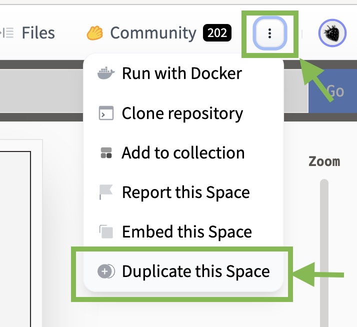 You'll observe that the Space owner, name, and visibility are already filled in for you, so you can leave those values as is. Your copy of the Space will run inside a Docker container that doesn't require many resources, so you can use the smallest instance. The official AI Comic Factory Space utilizes a bigger CPU instance, as it caters to a large user base. To operate the AI Comic Factory under your account, you need to configure your Hugging Face token: 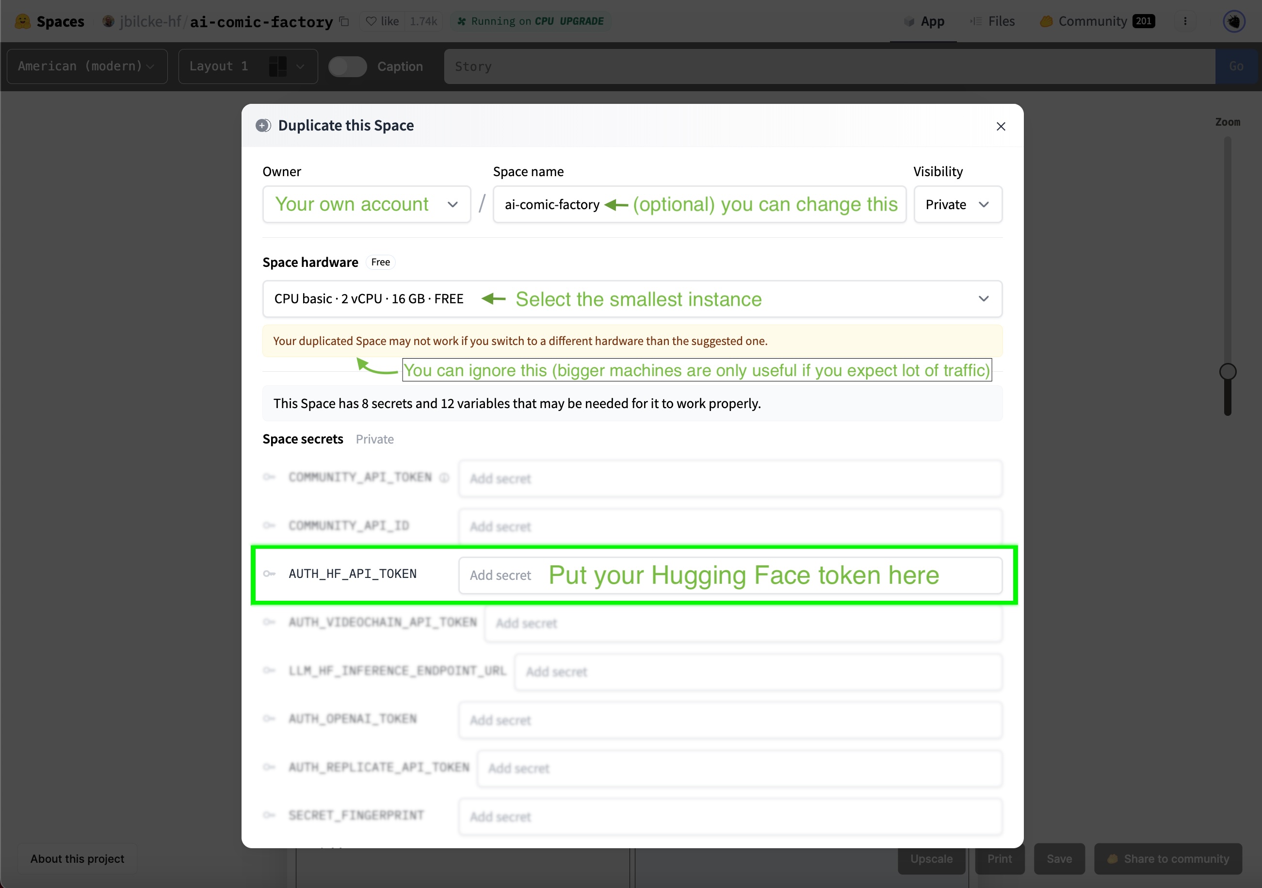 ## Selecting the LLM and SD engines The AI Comic Factory supports various backend engines, which can be configured using two environment variables: - `LLM_ENGINE` to configure the language model (possible values are `INFERENCE_API`, `INFERENCE_ENDPOINT`, `OPENAI`) - `RENDERING_ENGINE` to configure the image generation engine (possible values are `INFERENCE_API`, `INFERENCE_ENDPOINT`, `REPLICATE`, `VIDEOCHAIN`). We'll focus on making the AI Comic Factory work on the Inference API, so they both need to be set to `INFERENCE_API`:  You can find more information about alternative engines and vendors in the project's [README](https://huggingface.co/spaces/jbilcke-hf/ai-comic-factory/blob/main/README.md) and the [.env](https://huggingface.co/spaces/jbilcke-hf/ai-comic-factory/blob/main/README.md) config file. ## Configuring the models The AI Comic Factory comes with the following models pre-configured: - `LLM_HF_INFERENCE_API_MODEL`: default value is `meta-llama/Llama-2-70b-chat-hf` - `RENDERING_HF_RENDERING_INFERENCE_API_MODEL`: default value is `stabilityai/stable-diffusion-xl-base-1.0` Your PRO Hugging Face account already gives you access to those models, so you don't have anything to do or change. ## Going further Support for the Inference API in the AI Comic Factory is in its early stages, and some features, such as using the refiner step for SDXL or implementing upscaling, haven't been ported over yet. Nonetheless, we hope this information will enable you to start forking and tweaking the AI Comic Factory to suit your requirements. Feel free to experiment and try other models from the community, and happy hacking!"
Chat Templates: An End to the Silent Performance Killer,rocketknight1,"October 3, 2023",chat-templates,"LLM, nlp, community",https://huggingface.co/blog/chat-templates," # Chat Templates > *A spectre is haunting chat models - the spectre of incorrect formatting!* ## tl;dr Chat models have been trained with very different formats for converting conversations into a single tokenizable string. Using a format different from the format a model was trained with will usually cause severe, silent performance degradation, so matching the format used during training is extremely important! Hugging Face tokenizers now have a `chat_template` attribute that can be used to save the chat format the model was trained with. This attribute contains a Jinja template that converts conversation histories into a correctly formatted string. Please see the [technical documentation](https://huggingface.co/docs/transformers/main/en/chat_templating) for information on how to write and apply chat templates in your code. ## Introduction If you're familiar with the 🤗 Transformers library, you've probably written code like this: ```python tokenizer = AutoTokenizer.from_pretrained(checkpoint) model = AutoModel.from_pretrained(checkpoint) ``` By loading the tokenizer and model from the same checkpoint, you ensure that inputs are tokenized in the way the model expects. If you pick a tokenizer from a different model, the input tokenization might be completely different, and the result will be that your model's performance will be seriously damaged. The term for this is a **distribution shift** - the model has been learning data from one distribution (the tokenization it was trained with), and suddenly it has shifted to a completely different one. Whether you're fine-tuning a model or using it directly for inference, it's always a good idea to minimize these distribution shifts and keep the input you give it as similar as possible to the input it was trained on. With regular language models, it's relatively easy to do that - simply load your tokenizer and model from the same checkpoint, and you're good to go. With chat models, however, it's a bit different. This is because ""chat"" is not just a single string of text that can be straightforwardly tokenized - it's a sequence of messages, each of which contains a `role` as well as `content`, which is the actual text of the message. Most commonly, the roles are ""user"" for messages sent by the user, ""assistant"" for responses written by the model, and optionally ""system"" for high-level directives given at the start of the conversation. If that all seems a bit abstract, here's an example chat to make it more concrete: ```python [ {""role"": ""user"", ""content"": ""Hi there!""}, {""role"": ""assistant"", ""content"": ""Nice to meet you!""} ] ``` This sequence of messages needs to be converted into a text string before it can be tokenized and used as input to a model. The problem, though, is that there are many ways to do this conversion! You could, for example, convert the list of messages into an ""instant messenger"" format: ``` User: Hey there! Bot: Nice to meet you! ``` Or you could add special tokens to indicate the roles: ``` [USER] Hey there! [/USER] [ASST] Nice to meet you! [/ASST] ``` Or you could add tokens to indicate the boundaries between messages, but insert the role information as a string: ``` <|im_start|>user Hey there!<|im_end|> <|im_start|>assistant Nice to meet you!<|im_end|> ``` There are lots of ways to do this, and none of them is obviously the best or correct way to do it. As a result, different models have been trained with wildly different formatting. I didn't make these examples up; they're all real and being used by at least one active model! But once a model has been trained with a certain format, you really want to ensure that future inputs use the same format, or else you could get a performance-destroying distribution shift. ## Templates: A way to save format information Right now, if you're lucky, the format you need is correctly documented somewhere in the model card. If you're unlucky, it isn't, so good luck if you want to use that model. In extreme cases, we've even put the whole prompt format in [a blog post](https://huggingface.co/blog/llama2#how-to-prompt-llama-2) to ensure that users don't miss it! Even in the best-case scenario, though, you have to locate the template information and manually code it up in your fine-tuning or inference pipeline. We think this is an especially dangerous issue because using the wrong chat format is a **silent error** - you won't get a loud failure or a Python exception to tell you something is wrong, the model will just perform much worse than it would have with the right format, and it'll be very difficult to debug the cause! This is the problem that **chat templates** aim to solve. Chat templates are [Jinja template strings](https://jinja.palletsprojects.com/en/3.1.x/) that are saved and loaded with your tokenizer, and that contain all the information needed to turn a list of chat messages into a correctly formatted input for your model. Here are three chat template strings, corresponding to the three message formats above: ```jinja {% for message in messages %} {% if message['role'] == 'user' %} {{ ""User : "" }} {% else %} {{ ""Bot : "" }} {{ message['content'] + '\n' }} {% endfor %} ``` ```jinja {% for message in messages %} {% if message['role'] == 'user' %} {{ ""[USER] "" + message['content'] + "" [/USER]"" }} {% else %} {{ ""[ASST] "" + message['content'] + "" [/ASST]"" }} {{ message['content'] + '\n' }} {% endfor %} ``` ```jinja ""{% for message in messages %}"" ""{{'<|im_start|>' + message['role'] + '\n' + message['content'] + '<|im_end|>' + '\n'}}"" ""{% endfor %}"" ``` If you're unfamiliar with Jinja, I strongly recommend that you take a moment to look at these template strings, and their corresponding template outputs, and see if you can convince yourself that you understand how the template turns a list of messages into a formatted string! The syntax is very similar to Python in a lot of ways. ## Why templates? Although Jinja can be confusing at first if you're unfamiliar with it, in practice we find that Python programmers can pick it up quickly. During development of this feature, we considered other approaches, such as a limited system to allow users to specify per-role prefixes and suffixes for messages. We found that this could become confusing and unwieldy, and was so inflexible that hacky workarounds were needed for several models. Templating, on the other hand, is powerful enough to cleanly support all of the message formats that we're aware of. ## Why bother doing this? Why not just pick a standard format? This is an excellent idea! Unfortunately, it's too late, because multiple important models have already been trained with very different chat formats. However, we can still mitigate this problem a bit. We think the closest thing to a 'standard' for formatting is the [ChatML format](https://github.com/openai/openai-python/blob/main/chatml.md) created by OpenAI. If you're training a new model for chat, and this format is suitable for you, we recommend using it and adding special `<|im_start|>` and `<|im_end|>` tokens to your tokenizer. It has the advantage of being very flexible with roles, as the role is just inserted as a string rather than having specific role tokens. If you'd like to use this one, it's the third of the templates above, and you can set it with this simple one-liner: ```py tokenizer.chat_template = ""{% for message in messages %}{{'<|im_start|>' + message['role'] + '\n' + message['content'] + '<|im_end|>' + '\n'}}{% endfor %}"" ``` There's also a second reason not to hardcode a standard format, though, beyond the proliferation of existing formats - we expect that templates will be broadly useful in preprocessing for many types of models, including those that might be doing very different things from standard chat. Hardcoding a standard format limits the ability of model developers to use this feature to do things we haven't even thought of yet, whereas templating gives users and developers maximum freedom. It's even possible to encode checks and logic in templates, which is a feature we don't use extensively in any of the default templates, but which we expect to have enormous power in the hands of adventurous users. We strongly believe that the open-source ecosystem should enable you to do what you want, not dictate to you what you're permitted to do. ## How do templates work? Chat templates are part of the **tokenizer**, because they fulfill the same role as tokenizers do: They store information about how data is preprocessed, to ensure that you feed data to the model in the same format that it saw during training. We have designed it to be very easy to add template information to an existing tokenizer and save it or upload it to the Hub. Before chat templates, chat formatting information was stored at the **class level** - this meant that, for example, all LLaMA checkpoints would get the same chat formatting, using code that was hardcoded in `transformers` for the LLaMA model class. For backward compatibility, model classes that had custom chat format methods have been given **default chat templates** instead. Default chat templates are also set at the class level, and tell classes like `ConversationPipeline` how to format inputs when the model does not have a chat template. We're doing this **purely for backwards compatibility** - we highly recommend that you explicitly set a chat template on any chat model, even when the default chat template is appropriate. This ensures that any future changes or deprecations in the default chat template don't break your model. Although we will be keeping default chat templates for the foreseeable future, we hope to transition all models to explicit chat templates over time, at which point the default chat templates may be removed entirely. For information about how to set and apply chat templates, please see the [technical documentation](https://huggingface.co/docs/transformers/main/en/chat_templating). ## How do I get started with templates? Easy! If a tokenizer has the `chat_template` attribute set, it's ready to go. You can use that model and tokenizer in `ConversationPipeline`, or you can call `tokenizer.apply_chat_template()` to format chats for inference or training. Please see our [developer guide](https://huggingface.co/docs/transformers/main/en/chat_templating) or the [apply_chat_template documentation](https://huggingface.co/docs/transformers/main/en/internal/tokenization_utils#transformers.PreTrainedTokenizerBase.apply_chat_template) for more! If a tokenizer doesn't have a `chat_template` attribute, it might still work, but it will use the default chat template set for that model class. This is fragile, as we mentioned above, and it's also a source of silent bugs when the class template doesn't match what the model was actually trained with. If you want to use a checkpoint that doesn't have a `chat_template`, we recommend checking docs like the model card to verify what the right format is, and then adding a correct `chat_template`for that format. We recommend doing this even if the default chat template is correct - it future-proofs the model, and also makes it clear that the template is present and suitable. You can add a `chat_template` even for checkpoints that you're not the owner of, by opening a [pull request](https://huggingface.co/docs/hub/repositories-pull-requests-discussions). The only change you need to make is to set the `tokenizer.chat_template` attribute to a Jinja template string. Once that's done, push your changes and you're ready to go! If you'd like to use a checkpoint for chat but you can't find any documentation on the chat format it used, you should probably open an issue on the checkpoint or ping the owner! Once you figure out the format the model is using, please open a pull request to add a suitable `chat_template`. Other users will really appreciate it! ## Conclusion: Template philosophy We think templates are a very exciting change. In addition to resolving a huge source of silent, performance-killing bugs, we think they open up completely new approaches and data modalities. Perhaps most importantly, they also represent a philosophical shift: They take a big function out of the core `transformers` codebase and move it into individual model repos, where users have the freedom to do weird and wild and wonderful things. We're excited to see what uses you find for them!"
Accelerating Stable Diffusion XL Inference with JAX on Cloud TPU v5e,pcuenq,"October 3, 2023",sdxl_jax,"sdxl, jax, stable diffusion, guide, tpu, google",https://huggingface.co/blog/sdxl_jax," # Accelerating Stable Diffusion XL Inference with JAX on Cloud TPU v5e Generative AI models, such as Stable Diffusion XL (SDXL), enable the creation of high-quality, realistic content with wide-ranging applications. However, harnessing the power of such models presents significant challenges and computational costs. SDXL is a large image generation model whose UNet component is about three times as large as the one in the previous version of the model. Deploying a model like this in production is challenging due to the increased memory requirements, as well as increased inference times. Today, we are thrilled to announce that Hugging Face Diffusers now supports serving SDXL using JAX on Cloud TPUs, enabling high-performance, cost-efficient inference. [Google Cloud TPUs](https://cloud.google.com/tpu) are custom-designed AI accelerators, which are optimized for training and inference of large AI models, including state-of-the-art LLMs and generative AI models such as SDXL. The new [Cloud TPU v5e](https://cloud.google.com/blog/products/compute/announcing-cloud-tpu-v5e-and-a3-gpus-in-ga) is purpose-built to bring the cost-efficiency and performance required for large-scale AI [training](https://cloud.google.com/blog/products/compute/using-cloud-tpu-multislice-to-scale-ai-workloads) and [inference](https://cloud.google.com/blog/products/compute/how-cloud-tpu-v5e-accelerates-large-scale-ai-inference). At less than half the cost of TPU v4, TPU v5e makes it possible for more organizations to train and deploy AI models. 🧨 Diffusers JAX integration offers a convenient way to run SDXL on TPU via [XLA](https://github.com/openxla/xla), and we built a demo to showcase it. You can try it out in [this Space](https://huggingface.co/spaces/google/sdxl) or in the playground embedded below: Under the hood, this demo runs on several TPU v5e-4 instances (each instance has 4 TPU chips) and takes advantage of parallelization to serve four large 1024×1024 images in about 4 seconds. This time includes format conversions, communications time, and frontend processing; the actual generation time is about 2.3s, as we'll see below! In this blog post, 1. [We describe why JAX + TPU + Diffusers is a powerful framework to run SDXL](#why-jax--tpu-v5e-for-sdxl) 2. [Explain how you can write a simple image generation pipeline with Diffusers and JAX](#how-to-write-an-image-generation-pipeline-in-jax) 3. [Show benchmarks comparing different TPU settings](#benchmark) ## Why JAX + TPU v5e for SDXL? Serving SDXL with JAX on Cloud TPU v5e with high performance and cost-efficiency is possible thanks to the combination of purpose-built TPU hardware and a software stack optimized for performance. Below we highlight two key factors: JAX just-in-time (jit) compilation and XLA compiler-driven parallelism with JAX pmap. #### JIT compilation A notable feature of JAX is its [just-in-time (jit) compilation](https://jax.readthedocs.io/en/latest/jax-101/02-jitting.html). The JIT compiler traces code during the first run and generates highly optimized TPU binaries that are re-used in subsequent calls. The catch of this process is that it requires all input, intermediate, and output shapes to be **static**, meaning that they must be known in advance. Every time we change the shapes a new and costly compilation process will be triggered again. JIT compilation is ideal for services that can be designed around static shapes: compilation runs once, and then we take advantage of super-fast inference times. Image generation is well-suited for JIT compilation. If we always generate the same number of images and they have the same size, then the output shapes are constant and known in advance. The text inputs are also constant: by design, Stable Diffusion and SDXL use fixed-shape embedding vectors (with padding) to represent the prompts typed by the user. Therefore, we can write JAX code that relies on fixed shapes, and that can be greatly optimized! #### High-performance throughput for high batch sizes Workloads can be scaled across multiple devices using JAX's [pmap](https://jax.readthedocs.io/en/latest/_autosummary/jax.pmap.html), which expresses single-program multiple-data (SPMD) programs. Applying pmap to a function will compile a function with XLA, then execute it in parallel on various XLA devices. For text-to-image generation workloads this means that increasing the number of images rendered simultaneously is straightforward to implement and doesn't compromise performance. For example, running SDXL on a TPU with 8 chips will generate 8 images in the same time it takes for 1 chip to create a single image. TPU v5e instances come in multiple shapes, including 1, 4 and 8-chip shapes, all the way up to 256 chips (a full TPU v5e pod), with ultra-fast ICI links between chips. This allows you to choose the TPU shape that best suits your use case and easily take advantage of the parallelism that JAX and TPUs provide. ## How to write an image generation pipeline in JAX We'll go step by step over the code you need to write to run inference super-fast using JAX! First, let's import the dependencies. ```python # Show best practices for SDXL JAX import jax import jax.numpy as jnp import numpy as np from flax.jax_utils import replicate from diffusers import FlaxStableDiffusionXLPipeline import time ``` We'll now load the base SDXL model and the rest of the components required for inference. The diffusers pipeline takes care of downloading and caching everything for us. Adhering to JAX's functional approach, the model's parameters are returned separately and will have to be passed to the pipeline during inference: ```python pipeline, params = FlaxStableDiffusionXLPipeline.from_pretrained( ""stabilityai/stable-diffusion-xl-base-1.0"", split_head_dim=True ) ``` Model parameters are downloaded in 32-bit precision by default. To save memory and run computation faster we'll convert them to `bfloat16`, an efficient 16-bit representation. However, there's a caveat: for best results, we have to keep the _scheduler state_ in `float32`, otherwise precision errors accumulate and result in low-quality or even black images. ```python scheduler_state = params.pop(""scheduler"") params = jax.tree_util.tree_map(lambda x: x.astype(jnp.bfloat16), params) params[""scheduler""] = scheduler_state ``` We are now ready to set up our prompt and the rest of the pipeline inputs. ```python default_prompt = ""high-quality photo of a baby dolphin playing in a pool and wearing a party hat"" default_neg_prompt = ""illustration, low-quality"" default_seed = 33 default_guidance_scale = 5.0 default_num_steps = 25 ``` The prompts have to be supplied as tensors to the pipeline, and they always have to have the same dimensions across invocations. This allows the inference call to be compiled. The pipeline `prepare_inputs` method performs all the necessary steps for us, so we'll create a helper function to prepare both our prompt and negative prompt as tensors. We'll use it later from our `generate` function: ```python def tokenize_prompt(prompt, neg_prompt): prompt_ids = pipeline.prepare_inputs(prompt) neg_prompt_ids = pipeline.prepare_inputs(neg_prompt) return prompt_ids, neg_prompt_ids ``` To take advantage of parallelization, we'll replicate the inputs across devices. A Cloud TPU v5e-4 has 4 chips, so by replicating the inputs we get each chip to generate a different image, in parallel. We need to be careful to supply a different random seed to each chip so the 4 images are different: ```python NUM_DEVICES = jax.device_count() # Model parameters don't change during inference, # so we only need to replicate them once. p_params = replicate(params) def replicate_all(prompt_ids, neg_prompt_ids, seed): p_prompt_ids = replicate(prompt_ids) p_neg_prompt_ids = replicate(neg_prompt_ids) rng = jax.random.PRNGKey(seed) rng = jax.random.split(rng, NUM_DEVICES) return p_prompt_ids, p_neg_prompt_ids, rng ``` We are now ready to put everything together in a generate function: ```python def generate( prompt, negative_prompt, seed=default_seed, guidance_scale=default_guidance_scale, num_inference_steps=default_num_steps, ): prompt_ids, neg_prompt_ids = tokenize_prompt(prompt, negative_prompt) prompt_ids, neg_prompt_ids, rng = replicate_all(prompt_ids, neg_prompt_ids, seed) images = pipeline( prompt_ids, p_params, rng, num_inference_steps=num_inference_steps, neg_prompt_ids=neg_prompt_ids, guidance_scale=guidance_scale, jit=True, ).images # convert the images to PIL images = images.reshape((images.shape[0] * images.shape[1], ) + images.shape[-3:]) return pipeline.numpy_to_pil(np.array(images)) ``` `jit=True` indicates that we want the pipeline call to be compiled. This will happen the first time we call `generate`, and it will be very slow – JAX needs to trace the operations, optimize them, and convert them to low-level primitives. We'll run a first generation to complete this process and warm things up: ```python start = time.time() print(f""Compiling ..."") generate(default_prompt, default_neg_prompt) print(f""Compiled in {time.time() - start}"") ``` This took about three minutes the first time we ran it. But once the code has been compiled, inference will be super fast. Let's try again! ```python start = time.time() prompt = ""llama in ancient Greece, oil on canvas"" neg_prompt = ""cartoon, illustration, animation"" images = generate(prompt, neg_prompt) print(f""Inference in {time.time() - start}"") ``` It now took about 2s to generate the 4 images! ## Benchmark The following measures were obtained running SDXL 1.0 base for 20 steps, with the default Euler Discrete scheduler. We compare Cloud TPU v5e with TPUv4 for the same batch sizes. Do note that, due to parallelism, a TPU v5e-4 like the ones we use in our demo will generate **4 images** when using a batch size of 1 (or 8 images with a batch size of 2). Similarly, a TPU v5e-8 will generate 8 images when using a batch size of 1. The Cloud TPU tests were run using Python 3.10 and jax version 0.4.16. These are the same specs used in our [demo Space](https://huggingface.co/spaces/google/sdxl). | | Batch Size | Latency | Perf/$ | |-----------------|------------|:--------:|--------| | TPU v5e-4 (JAX) | 4 | 2.33s | 21.46 | | | 8 | 4.99s | 20.04 | | TPU v4-8 (JAX) | 4 | 2.16s | 9.05 | | | 8 | 4.17 | 8.98 | TPU v5e achieves up to 2.4x greater perf/$ on SDXL compared to TPU v4, demonstrating the cost-efficiency of the latest TPU generation. To measure inference performance, we use the industry-standard metric of throughput. First, we measure latency per image when the model has been compiled and loaded. Then, we calculate throughput by dividing batch size over latency per chip. As a result, throughput measures how the model is performing in production environments regardless of how many chips are used. We then divide throughput by the list price to get performance per dollar. ## How does the demo work? The [demo we showed before](https://huggingface.co/spaces/google/sdxl) was built using a script that essentially follows the code we posted in this blog post. It runs on a few Cloud TPU v5e devices with 4 chips each, and there's a simple load-balancing server that routes user requests to backend servers randomly. When you enter a prompt in the demo, your request will be assigned to one of the backend servers, and you'll receive the 4 images it generates. This is a simple solution based on several pre-allocated TPU instances. In a future post, we'll cover how to create dynamic solutions that adapt to load using GKE. All the code for the demo is open-source and available in Hugging Face Diffusers today. We are excited to see what you build with Diffusers + JAX + Cloud TPUs!"
"Accelerating over 130,000 Hugging Face models with ONNX Runtime",sschoenmeyer,"October 4, 2023",ort-accelerating-hf-models,"open-source-collab, onnxruntime, onnx, inference",https://huggingface.co/blog/ort-accelerating-hf-models," # Accelerating over 130,000 Hugging Face models with ONNX Runtime ## What is ONNX Runtime? ONNX Runtime is a cross-platform machine learning tool that can be used to accelerate a wide variety of models, particularly those with ONNX support. ## Hugging Face ONNX Runtime Support There are over 130,000 ONNX-supported models on Hugging Face, an open source community that allows users to build, train, and deploy hundreds of thousands of publicly available machine learning models. These ONNX-supported models, which include many increasingly popular large language models (LLMs) and cloud models, can leverage ONNX Runtime to improve performance, along with other benefits. For example, using ONNX Runtime to accelerate the whisper-tiny model can improve average latency per inference, with an up to 74.30% gain over PyTorch. ONNX Runtime works closely with Hugging Face to ensure that the most popular models on the site are supported. In total, over 90 Hugging Face model architectures are supported by ONNX Runtime, including the 11 most popular architectures (where popularity is determined by the corresponding number of models uploaded to the Hugging Face Hub): | Model Architecture | Approximate No. of Models | |:------------------:|:-------------------------:| | BERT | 28180 | | GPT2 | 14060 | | DistilBERT | 11540 | | RoBERTa | 10800 | | T5 | 10450 | | Wav2Vec2 | 6560 | | Stable-Diffusion | 5880 | | XLM-RoBERTa | 5100 | | Whisper | 4400 | | BART | 3590 | | Marian | 2840 | ## Learn More To learn more about accelerating Hugging Face models with ONNX Runtime, check out our recent post on the [Microsoft Open Source Blog](https://cloudblogs.microsoft.com/opensource/2023/10/04/accelerating-over-130000-hugging-face-models-with-onnx-runtime/)."
Gradio-Lite: Serverless Gradio Running Entirely in Your Browser,abidlabs,"October 19, 2023",gradio-lite,"gradio, open-source, serverless",https://huggingface.co/blog/gradio-lite," # Gradio-Lite: Serverless Gradio Running Entirely in Your Browser Gradio is a popular Python library for creating interactive machine learning apps. Traditionally, Gradio applications have relied on server-side infrastructure to run, which can be a hurdle for developers who need to host their applications. Enter Gradio-lite (`@gradio/lite`): a library that leverages [Pyodide](https://pyodide.org/en/stable/) to bring Gradio directly to your browser. In this blog post, we'll explore what `@gradio/lite` is, go over example code, and discuss the benefits it offers for running Gradio applications. ## What is `@gradio/lite`? `@gradio/lite` is a JavaScript library that enables you to run Gradio applications directly within your web browser. It achieves this by utilizing Pyodide, a Python runtime for WebAssembly, which allows Python code to be executed in the browser environment. With `@gradio/lite`, you can **write regular Python code for your Gradio applications**, and they will **run seamlessly in the browser** without the need for server-side infrastructure. ## Getting Started Let's build a ""Hello World"" Gradio app in `@gradio/lite` ### 1. Import JS and CSS Start by creating a new HTML file, if you don't have one already. Importing the JavaScript and CSS corresponding to the `@gradio/lite` package by using the following code: ```html ``` Note that you should generally use the latest version of `@gradio/lite` that is available. You can see the [versions available here](https://www.jsdelivr.com/package/npm/@gradio/lite?tab=files). ### 2. Create the `` tags Somewhere in the body of your HTML page (wherever you'd like the Gradio app to be rendered), create opening and closing `` tags. ```html ``` Note: you can add the `theme` attribute to the `` tag to force the theme to be dark or light (by default, it respects the system theme). E.g. ```html ... ``` ### 3. Write your Gradio app inside of the tags Now, write your Gradio app as you would normally, in Python! Keep in mind that since this is Python, whitespace and indentations matter. ```html import gradio as gr def greet(name): return ""Hello, "" + name + ""!"" gr.Interface(greet, ""textbox"", ""textbox"").launch() ``` And that's it! You should now be able to open your HTML page in the browser and see the Gradio app rendered! Note that it may take a little while for the Gradio app to load initially since Pyodide can take a while to install in your browser. **Note on debugging**: to see any errors in your Gradio-lite application, open the inspector in your web browser. All errors (including Python errors) will be printed there. ## More Examples: Adding Additional Files and Requirements What if you want to create a Gradio app that spans multiple files? Or that has custom Python requirements? Both are possible with `@gradio/lite`! ### Multiple Files Adding multiple files within a `@gradio/lite` app is very straightforward: use the `` tag. You can have as many `` tags as you want, but each one needs to have a `name` attribute and the entry point to your Gradio app should have the `entrypoint` attribute. Here's an example: ```html import gradio as gr from utils import add demo = gr.Interface(fn=add, inputs=[""number"", ""number""], outputs=""number"") demo.launch() def add(a, b): return a + b ``` ### Additional Requirements If your Gradio app has additional requirements, it is usually possible to [install them in the browser using micropip](https://pyodide.org/en/stable/usage/loading-packages.html#loading-packages). We've created a wrapper to make this paticularly convenient: simply list your requirements in the same syntax as a `requirements.txt` and enclose them with `` tags. Here, we install `transformers_js_py` to run a text classification model directly in the browser! ```html transformers_js_py from transformers_js import import_transformers_js import gradio as gr transformers = await import_transformers_js() pipeline = transformers.pipeline pipe = await pipeline('sentiment-analysis') async def classify(text): return await pipe(text) demo = gr.Interface(classify, ""textbox"", ""json"") demo.launch() ``` **Try it out**: You can see this example running in [this Hugging Face Static Space](https://huggingface.co/spaces/abidlabs/gradio-lite-classify), which lets you host static (serverless) web applications for free. Visit the page and you'll be able to run a machine learning model without internet access! ## Benefits of Using `@gradio/lite` ### 1. Serverless Deployment The primary advantage of @gradio/lite is that it eliminates the need for server infrastructure. This simplifies deployment, reduces server-related costs, and makes it easier to share your Gradio applications with others. ### 2. Low Latency By running in the browser, @gradio/lite offers low-latency interactions for users. There's no need for data to travel to and from a server, resulting in faster responses and a smoother user experience. ### 3. Privacy and Security Since all processing occurs within the user's browser, `@gradio/lite` enhances privacy and security. User data remains on their device, providing peace of mind regarding data handling. ### Limitations * Currently, the biggest limitation in using `@gradio/lite` is that your Gradio apps will generally take more time (usually 5-15 seconds) to load initially in the browser. This is because the browser needs to load the Pyodide runtime before it can render Python code. * Not every Python package is supported by Pyodide. While `gradio` and many other popular packages (including `numpy`, `scikit-learn`, and `transformers-js`) can be installed in Pyodide, if your app has many dependencies, its worth checking whether the dependencies are included in Pyodide, or can be [installed with `micropip`](https://micropip.pyodide.org/en/v0.2.2/project/api.html#micropip.install). ## Try it out! You can immediately try out `@gradio/lite` by copying and pasting this code in a local `index.html` file and opening it with your browser: ```html import gradio as gr def greet(name): return ""Hello, "" + name + ""!"" gr.Interface(greet, ""textbox"", ""textbox"").launch() ``` We've also created a playground on the Gradio website that allows you to interactively edit code and see the results immediately! Playground: https://www.gradio.app/playground "
Exploring simple optimizations for SDXL,sayakpaul,"October 24, 2023",simple_sdxl_optimizations,"diffusers, guide, sdxl",https://huggingface.co/blog/simple_sdxl_optimizations," # Exploring simple optimizations for SDXL ![]() [Stable Diffusion XL (SDXL)](https://huggingface.co/papers/2307.01952) is the latest latent diffusion model by Stability AI for generating high-quality super realistic images. It overcomes challenges of previous Stable Diffusion models like getting hands and text right as well as spatially correct compositions. In addition, SDXL is also more context aware and requires fewer words in its prompt to generate better looking images. However, all of these improvements come at the expense of a significantly larger model. How much larger? The base SDXL model has 3.5B parameters (the UNet, in particular), which is approximately 3x larger than the previous Stable Diffusion model. To explore how we can optimize SDXL for inference speed and memory use, we ran some tests on an A100 GPU (40 GB). For each inference run, we generate 4 images and repeat it 3 times. While computing the inference latency, we only consider the final iteration out of the 3 iterations. So if you run SDXL out-of-the-box as is with full precision and use the default attention mechanism, it’ll consume 28GB of memory and take 72.2 seconds! ```python from diffusers import StableDiffusionXLPipeline pipe = StableDiffusionXLPipeline.from_pretrained(""stabilityai/stable-diffusion-xl-base-1.0"").to(""cuda"") pipe.unet.set_default_attn_processor() ``` This isn’t very practical and can slow you down because you’re often generating more than 4 images. And if you don’t have a more powerful GPU, you’ll run into that frustrating out-of-memory error message. So how can we optimize SDXL to increase inference speed and reduce its memory-usage? In 🤗 Diffusers, we have a bunch of optimization tricks and techniques to help you run memory-intensive models like SDXL and we'll show you how! The two things we’ll focus on are *inference speed* and *memory*.
[Stable Diffusion XL (SDXL)](https://huggingface.co/papers/2307.01952) is the latest latent diffusion model by Stability AI for generating high-quality super realistic images. It overcomes challenges of previous Stable Diffusion models like getting hands and text right as well as spatially correct compositions. In addition, SDXL is also more context aware and requires fewer words in its prompt to generate better looking images. However, all of these improvements come at the expense of a significantly larger model. How much larger? The base SDXL model has 3.5B parameters (the UNet, in particular), which is approximately 3x larger than the previous Stable Diffusion model. To explore how we can optimize SDXL for inference speed and memory use, we ran some tests on an A100 GPU (40 GB). For each inference run, we generate 4 images and repeat it 3 times. While computing the inference latency, we only consider the final iteration out of the 3 iterations. So if you run SDXL out-of-the-box as is with full precision and use the default attention mechanism, it’ll consume 28GB of memory and take 72.2 seconds! ```python from diffusers import StableDiffusionXLPipeline pipe = StableDiffusionXLPipeline.from_pretrained(""stabilityai/stable-diffusion-xl-base-1.0"").to(""cuda"") pipe.unet.set_default_attn_processor() ``` This isn’t very practical and can slow you down because you’re often generating more than 4 images. And if you don’t have a more powerful GPU, you’ll run into that frustrating out-of-memory error message. So how can we optimize SDXL to increase inference speed and reduce its memory-usage? In 🤗 Diffusers, we have a bunch of optimization tricks and techniques to help you run memory-intensive models like SDXL and we'll show you how! The two things we’ll focus on are *inference speed* and *memory*. 🧠 The techniques discussed in this post are applicable to all the
pipelines.
⚠️ The first time you compile a model is slower, but once the model is compiled, all subsequent calls to it are much faster!
## Model memory footprint Models today are growing larger and larger, making it a challenge to fit them into memory. This section focuses on how you can reduce the memory footprint of these enormous models so you can run them on consumer GPUs. These techniques include CPU offloading, decoding latents into images over several steps rather than all at once, and using a distilled version of the autoencoder. ### Model CPU offloading Model offloading saves memory by loading the UNet into the GPU memory while the other components of the diffusion model (text encoders, VAE) are loaded onto the CPU. This way, the UNet can run for multiple iterations on the GPU until it is no longer needed. ```python from diffusers import StableDiffusionXLPipeline pipe = StableDiffusionXLPipeline.from_pretrained( ""stabilityai/stable-diffusion-xl-base-1.0"", torch_dtype=torch.float16, ).to(""cuda"") pipe.enable_model_cpu_offload() ``` Compared to the baseline, it now takes 20.2GB of memory which saves you 1.5GB of memory. ### Sequential CPU offloading Another type of offloading which can save you more memory at the expense of slower inference is sequential CPU offloading. Rather than offloading an entire model - like the UNet - model weights stored in different UNet submodules are offloaded to the CPU and only loaded onto the GPU right before the forward pass. Essentially, you’re only loading parts of the model each time which allows you to save even more memory. The only downside is that it is significantly slower because you’re loading and offloading submodules many times. ```python from diffusers import StableDiffusionXLPipeline pipe = StableDiffusionXLPipeline.from_pretrained( ""stabilityai/stable-diffusion-xl-base-1.0"", torch_dtype=torch.float16, ).to(""cuda"") pipe.enable_sequential_cpu_offload() ``` Compared to the baseline, this takes 19.9GB of memory but the inference time increases to 67 seconds. ## Slicing In SDXL, a variational encoder (VAE) decodes the refined latents (predicted by the UNet) into realistic images. The memory requirement of this step scales with the number of images being predicted (the batch size). Depending on the image resolution and the available GPU VRAM, it can be quite memory-intensive. This is where “slicing” is useful. The input tensor to be decoded is split into slices and the computation to decode it is completed over several steps. This saves memory and allows larger batch sizes. ```python pipe = StableDiffusionXLPipeline.from_pretrained( ""stabilityai/stable-diffusion-xl-base-1.0"", torch_dtype=torch.float16, ).to(""cuda"") pipe.enable_vae_slicing() ``` With sliced computations, we reduce the memory to 15.4GB. If we add sequential CPU offloading, it is further reduced to 11.45GB which lets you generate 4 images (1024x1024) per prompt. However, with sequential offloading, the inference latency also increases. ## Caching computations Any text-conditioned image generation model typically uses a text encoder to compute embeddings from the input prompt. SDXL uses *two* text encoders! This contributes quite a bit to the inference latency. However, since these embeddings remain unchanged throughout the reverse diffusion process, we can precompute them and reuse them as we go. This way, after computing the text embeddings, we can remove the text encoders from memory. First, load the text encoders and their corresponding tokenizers and compute the embeddings from the input prompt: ```python tokenizers = [tokenizer, tokenizer_2] text_encoders = [text_encoder, text_encoder_2] ( prompt_embeds, negative_prompt_embeds, pooled_prompt_embeds, negative_pooled_prompt_embeds ) = encode_prompt(tokenizers, text_encoders, prompt) ``` Next, flush the GPU memory to remove the text encoders: ```jsx del text_encoder, text_encoder_2, tokenizer, tokenizer_2 flush() ``` Now the embeddings are good to go straight to the SDXL pipeline: ```python from diffusers import StableDiffusionXLPipeline pipe = StableDiffusionXLPipeline.from_pretrained( ""stabilityai/stable-diffusion-xl-base-1.0"", text_encoder=None, text_encoder_2=None, tokenizer=None, tokenizer_2=None, torch_dtype=torch.float16, ).to(""cuda"") call_args = dict( prompt_embeds=prompt_embeds, negative_prompt_embeds=negative_prompt_embeds, pooled_prompt_embeds=pooled_prompt_embeds, negative_pooled_prompt_embeds=negative_pooled_prompt_embeds, num_images_per_prompt=num_images_per_prompt, num_inference_steps=num_inference_steps, ) image = pipe(**call_args).images[0] ``` Combined with SDPA and fp16, we can reduce the memory to 21.9GB. Other techniques discussed above for optimizing memory can also be used with cached computations. ## Tiny Autoencoder As previously mentioned, a VAE decodes latents into images. Naturally, this step is directly bottlenecked by the size of the VAE. So, let’s just use a smaller autoencoder! The [Tiny Autoencoder by `madebyollin`](https://github.com/madebyollin/taesd), available [the Hub](https://huggingface.co/madebyollin/taesdxl) is just 10MB and it is distilled from the original VAE used by SDXL. ```python from diffusers import AutoencoderTiny pipe = StableDiffusionXLPipeline.from_pretrained( ""stabilityai/stable-diffusion-xl-base-1.0"", torch_dtype=torch.float16, ) pipe.vae = AutoencoderTiny.from_pretrained(""madebyollin/taesdxl"", torch_dtype=torch.float16) pipe.to(""cuda"") ``` With this setup, we reduce the memory requirement to 15.6GB while reducing the inference latency at the same time. ⚠️ The Tiny Autoencoder can omit some of the more fine-grained details from images, which is why the Tiny AutoEncoder is more appropriate for image previews.
## Conclusion To conclude and summarize the savings from our optimizations: ⚠️ While profiling GPUs to measure the trade-off between inference latency and memory requirements, it is important to be aware of the hardware being used. The above findings may not translate equally from hardware to hardware. For example, `torch.compile` only seems to benefit modern GPUs, at least for SDXL.
| **Technique** | **Memory (GB)** | **Inference latency (ms)** | | --- | --- | --- | | unoptimized pipeline | 28.09 | 72200.5 | | fp16 | 21.72 | 14800.9 | | **fp16 + SDPA (default)** | **21.72** | **11413.0** | | default + `torch.compile` | 21.73 | 10296.7 | | default + model CPU offload | 20.21 | 16082.2 | | default + sequential CPU offload | 19.91 | 67034.0 | | **default + VAE slicing** | **15.40** | **11232.2** | | default + VAE slicing + sequential CPU offload | 11.47 | 66869.2 | | default + precomputed text embeddings | 21.85 | 11909.0 | | default + Tiny Autoencoder | 15.48 | 10449.7 | We hope these optimizations make it a breeze to run your favorite pipelines. Try these techniques out and share your images with us! 🤗 --- **Acknowledgements**: Thank you to [Pedro Cuenca](https://twitter.com/pcuenq?lang=en) for his helpful reviews on the draft."
The N Implementation Details of RLHF with PPO,vwxyzjn,"October 24, 2023",the_n_implementation_details_of_rlhf_with_ppo,"research, rl, rlhf",https://huggingface.co/blog/the_n_implementation_details_of_rlhf_with_ppo," # The N Implementation Details of RLHF with PPO RLHF / ChatGPT has been a popular research topic these days. In our quest to research more on RLHF, this blog post attempts to do a reproduction of OpenAI’s 2019 original RLHF codebase at [*openai/lm-human-preferences*](https://github.com/openai/lm-human-preferences). Despite its “tensorflow-1.x-ness,” OpenAI’s original codebase is very well-evaluated and benchmarked, making it a good place to study RLHF implementation engineering details. We aim to: 1. reproduce OAI’s results in stylistic tasks and match the learning curves of [*openai/lm-human-preferences*](https://github.com/openai/lm-human-preferences). 2. present a checklist of implementation details, similar to the spirit of [*The 37 Implementation Details of Proximal Policy Optimization*](https://iclr-blog-track.github.io/2022/03/25/ppo-implementation-details/); [*Debugging RL, Without the Agonizing Pain*](https://andyljones.com/posts/rl-debugging.html). 3. provide a simple-to-read and minimal reference implementation of RLHF; This work is just for educational / learning purposes. For advanced users requiring more features, such as running larger models with PEFT, [*huggingface/trl*](https://github.com/huggingface/trl) would be a great choice. - In [Matching Learning Curves](#matching-learning-curves), we show our main contribution: creating a codebase that can reproduce OAI’s results in the stylistic tasks and matching learning curves very closely with [*openai/lm-human-preferences*](https://github.com/openai/lm-human-preferences). - We then take a technical deep dive into the implementation details that are relevant to reproducing OAI’s work. In [General Implementation Details](#general-implementation-details), we talk about basic details, such as how rewards/values are generated and how responses are generated. In [Reward Model Implementation Details](#reward-model-implementation-details), we talk about details such as reward normalization. In [Policy Training Implementation Details](#policy-training-implementation-details), we discuss details such as rejection sampling and reward “whitening”. - In [**PyTorch Adam optimizer numerical issues w.r.t RLHF**](#pytorch-adam-optimizer-numerical-issues-wrt-rlhf), we highlight a very interesting implementation difference in Adam between TensorFlow and PyTorch, which causes an aggressive update in the model training. - Next, we examine the effect of training different base models (e.g., gpt2-xl, falcon-1b,) given that the reward labels are produced with `gpt2-large`. - Finally, we conclude our work with limitations and discussions. **Here are the important links:** - 💾 Our reproduction codebase [*https://github.com/vwxyzjn/lm-human-preference-details*](https://github.com/vwxyzjn/lm-human-preference-details) - 🤗 Demo of RLHF model comparison: [*https://huggingface.co/spaces/lm-human-preference-details/rlhf-demo*](https://huggingface.co/spaces/lm-human-preference-details/rlhf-demo) - 🐝 All w&b training logs [*https://wandb.ai/openrlbenchmark/lm_human_preference_details*](https://wandb.ai/openrlbenchmark/lm_human_preference_details) # Matching Learning Curves Our main contribution is to reproduce OAI’s results in stylistic tasks, such as sentiment and descriptiveness. As shown in the figure below, our codebase (orange curves) can produce nearly identical learning curves as OAI’s codebase (blue curves).  ## A note on running openai/lm-human-preferences To make a direct comparison, we ran the original RLHF code at [*openai/lm-human-preferences*](https://github.com/openai/lm-human-preferences), which will offer valuable metrics to help validate and diagnose our reproduction. We were able to set the original TensorFlow 1.x code up, but it requires a hyper-specific setup: - OAI’s dataset was partially corrupted/lost (so we replaced them with similar HF datasets, which may or may not cause a performance difference) - Specifically, its book dataset was lost during OpenAI’s GCP - Azure migration ([https://github.com/openai/lm-human-preferences/issues/17#issuecomment-1044051496](https://github.com/openai/lm-human-preferences/issues/17#issuecomment-1044051496)). I replaced the book dataset with Hugging Face’s `bookcorpus` dataset, which is, in principle, what OAI used. - It can’t run on 1 V100 because it doesn’t implement gradient accumulation. Instead, it uses a large batch size and splits the batch across 8 GPUs, and will OOM on just 1 GPU. - It can’t run on 8x A100 because it uses TensorFlow 1.x, which is incompatible with Cuda 8+ - It can’t run on 8x V100 (16GB) because it will OOM - It can only run on 8x V100 (32GB), which is only offered by AWS as the `p3dn.24xlarge` instance. # General Implementation Details We now take a technical deep dive into the implementation details that are relevant to reproducing OAI’s work. In this section, we talk about basic details, such as how rewards/values are generated and how responses are generated. Here are these details in no particular order: 1. **The reward model and policy’s value head take input as the concatenation of `query` and `response`** 1. The reward model and policy’s value head do *not* only look at the response. Instead, it concatenates the `query` and `response` together as `query_response` ([lm_human_preferences/rewards.py#L105-L107](https://github.com/openai/lm-human-preferences/blob/cbfd210bb8b08f6bc5c26878c10984b90f516c66/lm_human_preferences/rewards.py#L105-L107)). 2. So, for example, if `query = ""he was quiet for a minute, his eyes unreadable""`., and the `response = ""He looked at his left hand, which held the arm that held his arm out in front of him.""`, then the reward model and policy’s value do a forward pass on `query_response = ""he was quiet for a minute, his eyes unreadable. He looked at his left hand, which held the arm that held his arm out in front of him.""` and produced rewards and values of shape `(B, T, 1)`, where `B` is the batch size, `T` is the sequence length, and `1` is the reward head dimension of 1 ([lm_human_preferences/rewards.py#L105-L107](https://github.com/openai/lm-human-preferences/blob/cbfd210bb8b08f6bc5c26878c10984b90f516c66/lm_human_preferences/rewards.py#L105-L107), [lm_human_preferences/policy.py#L111](https://github.com/openai/lm-human-preferences/blob/cbfd210bb8b08f6bc5c26878c10984b90f516c66/lm_human_preferences/policy.py#L111)). 3. The `T` means that each token has a reward associated with it and its previous context. For example, the `eyes` token would have a reward corresponding to `he was quiet for a minute, his eyes`. 2. **Pad with a special padding token and truncate inputs.** 1. OAI sets a fixed input length for query `query_length`; it **pads** sequences that are too short with `pad_token` ([lm_human_preferences/language/datasets.py#L66-L67](https://github.com/openai/lm-human-preferences/blob/cbfd210bb8b08f6bc5c26878c10984b90f516c66/lm_human_preferences/language/datasets.py#L66-L67)) and **truncates** sequences that are too long ([lm_human_preferences/language/datasets.py#L57](https://github.com/openai/lm-human-preferences/blob/cbfd210bb8b08f6bc5c26878c10984b90f516c66/lm_human_preferences/language/datasets.py#L57)). See [here](https://huggingface.co/docs/transformers/pad_truncation) for a general introduction to the concept). When padding the inputs, OAI uses a token beyond the vocabulary ([lm_human_preferences/language/encodings.py#L56](https://github.com/openai/lm-human-preferences/blob/cbfd210bb8b08f6bc5c26878c10984b90f516c66/lm_human_preferences/language/encodings.py#L56)). 1. **Note on HF’s transformers — padding token.** According to ([transformers#2630#issuecomment-578159876](https://github.com/huggingface/transformers/issues/2630#issuecomment-578159876)), padding tokens were not used during the pre-training of GPT and GPT-2; therefore transformer’s gpt2 models have no official padding token associated with its tokenizer. A common practice is to set `tokenizer.pad_token = tokenizer.eos_token`, but in this work, we shall distinguish these two special tokens to match OAI’s original setting, so we will use `tokenizer.add_special_tokens({""pad_token"": ""[PAD]""})`. Note that having no padding token is a default setting for decoder models, since they train with “packing” during pretraining, which means that many sequences are concatenated and separated by the EOS token and chunks of this sequence that always have the max length are fed to the model during pretraining. 2. When putting everything together, here is an example ```python import transformers tokenizer = transformers.AutoTokenizer.from_pretrained(""gpt2"", padding_side=""right"") tokenizer.add_special_tokens({""pad_token"": ""[PAD]""}) query_length = 5 texts = [ ""usually, he would"", ""she thought about it"", ] tokens = [] for text in texts: tokens.append(tokenizer.encode(text)[:query_length]) print(""tokens"", tokens) inputs = tokenizer.pad( {""input_ids"": tokens}, padding=""max_length"", max_length=query_length, return_tensors=""pt"", return_attention_mask=True, ) print(""inputs"", inputs) """"""prints are tokens [[23073, 11, 339, 561], [7091, 1807, 546, 340]] inputs {'input_ids': tensor([[23073, 11, 339, 561, 50257], [ 7091, 1807, 546, 340, 50257]]), 'attention_mask': tensor([[1, 1, 1, 1, 0], [1, 1, 1, 1, 0]])} """""" ``` 3. **Adjust position indices correspondingly for padding tokens** 1. When calculating the logits, OAI’s code works by masking out padding tokens properly. This is achieved by finding out the token indices corresponding to the padding tokens ([lm_human_preferences/language/model.py#L296-L297](https://github.com/openai/lm-human-preferences/blob/cbfd210bb8b08f6bc5c26878c10984b90f516c66/lm_human_preferences/language/model.py#L296-L297)), followed by adjusting their position indices correspondingly ([lm_human_preferences/language/model.py#L320](https://github.com/openai/lm-human-preferences/blob/cbfd210bb8b08f6bc5c26878c10984b90f516c66/lm_human_preferences/language/model.py#L320)). 2. For example, if the `query=[23073, 50259, 50259]` and `response=[11, 339, 561]`, where (`50259` is OAI’s padding token), it then creates position indices as `[[0 1 1 1 2 3]]` and logits as follows. Note how the logits corresponding to the padding tokens remain the same as before! This is the effect we should be aiming for in our reproduction. ```python all_logits [[[ -35.28693 -34.2875 -38.16074 ... -41.595802 -41.082108 -35.36577 ] [ -35.28693 -34.2875 -38.16074 ... -41.595802 -41.082108 -35.36577 ] [ -35.28693 -34.2875 -38.16074 ... -41.595802 -41.082108 -35.36577 ] [-111.303955 -110.94471 -112.90624 ... -113.13064 -113.7788 -109.17345 ] [-111.51512 -109.61077 -114.90231 ... -118.43514 -111.56671 -112.12478 ] [-122.69775 -121.84468 -128.27417 ... -132.28055 -130.39604 -125.707756]]] (1, 6, 50257) ``` 3. **Note on HF’s transformers — `position_ids` and `padding_side`.** We can replicate the exact logits using Hugging Face’s transformer with 1) left padding and 2) pass in the appropriate `position_ids`: ```python import torch import transformers tokenizer = transformers.AutoTokenizer.from_pretrained(""gpt2"", padding_side=""right"") tokenizer.add_special_tokens({""pad_token"": ""[PAD]""}) pad_id = tokenizer.pad_token_id query = torch.tensor([ [pad_id, pad_id, 23073], ]) response = torch.tensor([ [11, 339, 561], ]) temperature = 1.0 query = torch.tensor(query) response = torch.tensor(response).long() context_length = query.shape[1] query_response = torch.cat((query, response), 1) pretrained_model = transformers.AutoModelForCausalLM.from_pretrained(""gpt2"") def forward(policy, query_responses, tokenizer): attention_mask = query_responses != tokenizer.pad_token_id position_ids = attention_mask.cumsum(1) - attention_mask.long() # exclusive cumsum input_ids = query_responses.clone() input_ids[~attention_mask] = 0 return policy( input_ids=input_ids, attention_mask=attention_mask, position_ids=position_ids, return_dict=True, output_hidden_states=True, ) output = forward(pretrained_model, query_response, tokenizer) logits = output.logits logits /= temperature print(logits) """""" tensor([[[ -26.9395, -26.4709, -30.0456, ..., -33.2208, -33.2884, -27.4360], [ -27.1677, -26.7330, -30.2386, ..., -33.6813, -33.6931, -27.5928], [ -35.2869, -34.2875, -38.1608, ..., -41.5958, -41.0821, -35.3658], [-111.3040, -110.9447, -112.9062, ..., -113.1306, -113.7788, -109.1734], [-111.5152, -109.6108, -114.9024, ..., -118.4352, -111.5668, -112.1248], [-122.6978, -121.8447, -128.2742, ..., -132.2805, -130.3961, -125.7078]]], grad_fn=) """""" ``` 4. **Note on HF’s transformers — `position_ids` during `generate`:** during generate we should not pass in `position_ids` because the `position_ids` are already adjusted in `transformers` (see [huggingface/transformers#/7552](https://github.com/huggingface/transformers/pull/7552). Usually, we almost never pass `position_ids` in transformers. All the masking and shifting logic are already implemented e.g. in the `generate` function (need permanent code link). 4. **Response generation samples a fixed-length response without padding.** 1. During response generation, OAI uses `top_k=0, top_p=1.0` and just do categorical samples across the vocabulary ([lm_human_preferences/language/sample.py#L43](https://github.com/openai/lm-human-preferences/blob/cbfd210bb8b08f6bc5c26878c10984b90f516c66/lm_human_preferences/language/sample.py#L43)) and the code would keep sampling until a fixed-length response is generated ([lm_human_preferences/policy.py#L103](https://github.com/openai/lm-human-preferences/blob/cbfd210bb8b08f6bc5c26878c10984b90f516c66/lm_human_preferences/policy.py#L103)). Notably, even if it encounters EOS (end-of-sequence) tokens, it will keep sampling. 2. **Note on HF’s transformers — sampling could stop at `eos_token`:** in `transformers`, the generation could stop at `eos_token` ([src/transformers/generation/utils.py#L2248-L2256](https://github.com/huggingface/transformers/blob/67b85f24def79962ce075353c2627f78e0e53e9f/src/transformers/generation/utils.py#L2248-L2256)), which is not the same as OAI’s setting. To align the setting, we need to do set `pretrained_model.generation_config.eos_token_id = None, pretrained_model.generation_config.pad_token_id = None`. Note that `transformers.GenerationConfig(eos_token_id=None, pad_token_id=None, ...)` does not work because `pretrained_model.generation_config` would override and set a `eos_token`. ```python import torch import transformers tokenizer = transformers.AutoTokenizer.from_pretrained(""gpt2"", padding_side=""right"") tokenizer.add_special_tokens({""pad_token"": ""[PAD]""}) pad_id = tokenizer.pad_token_id query = torch.tensor([ [pad_id, pad_id, 23073], ]) response = torch.tensor([ [11, 339, 561], ]) response_length = 4 temperature = 0.7 pretrained_model = transformers.AutoModelForCausalLM.from_pretrained(""gpt2"") pretrained_model.generation_config.eos_token_id = None # disable `pad_token_id` and `eos_token_id` because we just want to pretrained_model.generation_config.pad_token_id = None # generate tokens without truncation / padding generation_config = transformers.GenerationConfig( max_new_tokens=response_length, min_new_tokens=response_length, temperature=temperature, top_k=0.0, top_p=1.0, do_sample=True, ) context_length = query.shape[1] attention_mask = query != tokenizer.pad_token_id input_ids = query.clone() input_ids[~attention_mask] = 0 # set padding tokens to 0 output = pretrained_model.generate( input_ids=input_ids, attention_mask=attention_mask, # position_ids=attention_mask.cumsum(1) - attention_mask.long(), # generation collapsed if this was turned on. generation_config=generation_config, return_dict_in_generate=True, ) print(output.sequences) """""" tensor([[ 0, 0, 23073, 16851, 11, 475, 991]]) """""" ``` 3. Note that in a more recent codebase https://github.com/openai/summarize-from-feedback, OAI does stop sampling when encountering EOS token ([summarize_from_feedback/utils/experiment_helpers.py#L19](https://github.com/openai/summarize-from-feedback/blob/8af822a428c93432aa80ffbe5b065a8f93895669/summarize_from_feedback/utils/experiment_helpers.py#L19)). However in this work we aim to do a 1:1 replication, so we align the setting that could keep sampling even eos_token is encountered 5. **Learning rate annealing for reward model and policy training.** 1. As Ziegler et al. (2019) suggested, the reward model is trained for a single epoch to avoid overfitting the limited amount of human annotation data (e.g., the `descriptiveness` task only had about 5000 labels). During this single epoch, the learning rate is annealed to zero ([lm_human_preferences/train_reward.py#L249](https://github.com/openai/lm-human-preferences/blob/cbfd210bb8b08f6bc5c26878c10984b90f516c66/lm_human_preferences/train_reward.py#L249)). 2. Similar to reward model training, the learning rate is annealed to zero ([lm_human_preferences/train_policy.py#L172-L173](https://github.com/openai/lm-human-preferences/blob/cbfd210bb8b08f6bc5c26878c10984b90f516c66/lm_human_preferences/train_policy.py#L172-L173)). 6. **Use different seeds for different processes** 1. When spawning 8 GPU processes to do data parallelism, OAI sets a different random seed per process ([lm_human_preferences/utils/core.py#L108-L111](https://github.com/openai/lm-human-preferences/blob/cbfd210bb8b08f6bc5c26878c10984b90f516c66/lm_human_preferences/utils/core.py#L108-L111)). Implementation-wise, this is done via `local_seed = args.seed + process_rank * 100003`. The seed is going to make the model produce different responses and get different scores, for example. 1. Note: I believe the dataset shuffling has a bug — the dataset is shuffled using the same seed for some reason ([lm_human_preferences/lm_tasks.py#L94-L97](https://github.com/openai/lm-human-preferences/blob/cbfd210bb8b08f6bc5c26878c10984b90f516c66/lm_human_preferences/lm_tasks.py#L94-L97)). # Reward Model Implementation Details In this section, we discuss reward-model-specific implementation details. We talk about details such as reward normalization and layer initialization. Here are these details in no particular order: 1. **The reward model only outputs the value at the last token.** 1. Notice that the rewards obtained after the forward pass on the concatenation of `query` and `response` will have the shape `(B, T, 1)`, where `B` is the batch size, `T` is the sequence length (which is always the same; it is `query_length + response_length = 64 + 24 = 88` in OAI’s setting for stylistic tasks, see [launch.py#L9-L11](https://github.com/openai/lm-human-preferences/blob/cbfd210bb8b08f6bc5c26878c10984b90f516c66/launch.py#L9-L11)), and `1` is the reward head dimension of 1. For RLHF purposes, the original codebase extracts the reward of the last token ([lm_human_preferences/rewards.py#L132](https://github.com/openai/lm-human-preferences/blob/cbfd210bb8b08f6bc5c26878c10984b90f516c66/lm_human_preferences/rewards.py#L132)), so that the rewards will only have shape `(B, 1)`. 2. Note that in a more recent codebase [*openai/summarize-from-feedback*](https://github.com/openai/summarize-from-feedback), OAI stops sampling when encountering EOS token ([summarize_from_feedback/utils/experiment_helpers.py#L19](https://github.com/openai/summarize-from-feedback/blob/8af822a428c93432aa80ffbe5b065a8f93895669/summarize_from_feedback/utils/experiment_helpers.py#L19)). When extracting rewards, it is going to identify the `last_response_index`, the index before the EOS token ([#L11-L13](https://github.com/openai/summarize-from-feedback/blob/8af822a428c93432aa80ffbe5b065a8f93895669/summarize_from_feedback/reward_model.py#L11-L13)), and extract the reward at that index ([summarize_from_feedback/reward_model.py#L59](https://github.com/openai/summarize-from-feedback/blob/8af822a428c93432aa80ffbe5b065a8f93895669/summarize_from_feedback/reward_model.py#L59)). However in this work we just stick with the original setting. 2. **Reward head layer initialization** 1. The weight of the reward head is initialized according to \\( \mathcal{N}\left(0,1 /\left(\sqrt{d_{\text {model }}+1}\right)\right) \\) ([lm_human_preferences/language/model.py#L368,](https://github.com/openai/lm-human-preferences/blob/cbfd210bb8b08f6bc5c26878c10984b90f516c66/lm_human_preferences/language/model.py#L368) [lm_human_preferences/language/model.py#L251-L252](https://github.com/openai/lm-human-preferences/blob/cbfd210bb8b08f6bc5c26878c10984b90f516c66/lm_human_preferences/language/model.py#L251-L252)). This aligns with the settings in Stiennon et al., 2020 ([summarize_from_feedback/query_response_model.py#L106-L107](https://github.com/openai/summarize-from-feedback/blob/8af822a428c93432aa80ffbe5b065a8f93895669/summarize_from_feedback/query_response_model.py#L106-L107)) (P.S., Stiennon et al., 2020 had a typo on page 17 saying the distribution is \\( \mathcal{N}\left(0,1 /\left(d_{\text {model }}+1\right)\right) \\) without the square root) 2. The bias of the reward head is set to 0 ([lm_human_preferences/language/model.py#L254](https://github.com/openai/lm-human-preferences/blob/cbfd210bb8b08f6bc5c26878c10984b90f516c66/lm_human_preferences/language/model.py#L254)). 3. **Reward model normalization before and after** 1. In the paper, Ziegler el al. (2019) mentioned that ""to keep the scale of the reward model consistent across training, we normalize it so that it has mean 0 and variance 1 for \\( x \sim \mathcal{D}, y \sim \rho(·|x) \\).” To perform the normalization process, the code first creates a `reward_gain` and `reward_bias`, such that the reward can be calculated by `reward = reward * reward_gain + reward_bias` ([lm_human_preferences/rewards.py#L50-L51](https://github.com/openai/lm-human-preferences/blob/cbfd210bb8b08f6bc5c26878c10984b90f516c66/lm_human_preferences/rewards.py#L50-L51)). 2. When performing the normalization process, the code first sets `reward_gain=1, reward_bias=0` ([lm_human_preferences/train_reward.py#L211](https://github.com/openai/lm-human-preferences/blob/cbfd210bb8b08f6bc5c26878c10984b90f516c66/lm_human_preferences/train_reward.py#L211)), followed by collecting sampled queries from the target dataset (e.g., `bookcorpus, tldr, cnndm`), completed responses, and evaluated rewards. It then gets the **empirical mean and std** of the evaluated reward ([lm_human_preferences/train_reward.py#L162-L167](https://github.com/openai/lm-human-preferences/blob/cbfd210bb8b08f6bc5c26878c10984b90f516c66/lm_human_preferences/train_reward.py#L162-L167)) and tries to compute what the `reward_gain` and `reward_bias` should be. 3. Let us use \\( \mu_{\mathcal{D}} \\) to denote the empirical mean, \\( \sigma_{\mathcal{D}} \\) the empirical std, \\(g\\) the `reward_gain`, \\(b\\) `reward_bias`, \\( \mu_{\mathcal{T}} = 0\\) **target mean** and \\( \sigma_{\mathcal{T}}=1\\) **target std**. Then we have the following formula. $$\begin{aligned}g*\mathcal{N}(\mu_{\mathcal{D}}, \sigma_{\mathcal{D}}) + b &= \mathcal{N}(g*\mu_{\mathcal{D}}, g*\sigma_{\mathcal{D}}) + b\\&= \mathcal{N}(g*\mu_{\mathcal{D}} + b, g*\sigma_{\mathcal{D}}) \\&= \mathcal{N}(\mu_{\mathcal{T}}, \sigma_{\mathcal{T}}) \\g &= \frac{\sigma_{\mathcal{T}}}{\sigma_{\mathcal{D}}} \\b &= \mu_{\mathcal{T}} - g*\mu_{\mathcal{D}}\end{aligned}$$ 4. The normalization process is then applied **before** and **after** reward model training ([lm_human_preferences/train_reward.py#L232-L234](https://github.com/openai/lm-human-preferences/blob/cbfd210bb8b08f6bc5c26878c10984b90f516c66/lm_human_preferences/train_reward.py#L232-L234), [lm_human_preferences/train_reward.py#L252-L254](https://github.com/openai/lm-human-preferences/blob/cbfd210bb8b08f6bc5c26878c10984b90f516c66/lm_human_preferences/train_reward.py#L252-L254)). 5. Note that responses \\( y \sim \rho(·|x) \\) we generated for the normalization purpose are from the pre-trained language model \\(\rho \\). The model \\(\rho \\) is fixed as a reference and is not updated in reward learning ([lm_human_preferences/train_reward.py#L286C1-L286C31](https://github.com/openai/lm-human-preferences/blob/master/lm_human_preferences/train_reward.py#L286C1-L286C31)). # Policy Training Implementation Details In this section, we will delve into details, such as layer initialization, data post-processing, and dropout settings. We will also explore techniques, such as of rejection sampling and reward ""whitening"", and adaptive KL. Here are these details in no particular order: 1. **Scale the logits by sampling temperature.** 1. When calculating the log probability of responses, the model first outputs the logits of the tokens in the responses, followed by dividing the logits with the sampling temperature ([lm_human_preferences/policy.py#L121](https://github.com/openai/lm-human-preferences/blob/cbfd210bb8b08f6bc5c26878c10984b90f516c66/lm_human_preferences/policy.py#L121)). I.e., `logits /= self.temperature` 2. In an informal test, we found that without this scaling, the KL would rise faster than expected, and performance would deteriorate. 2. **Value head layer initialization** 1. The weight of the value head is initialized according to \\(\mathcal{N}\left(0,0\right)\\) ([lm_human_preferences/language/model.py#L368,](https://github.com/openai/lm-human-preferences/blob/cbfd210bb8b08f6bc5c26878c10984b90f516c66/lm_human_preferences/language/model.py#L368) [lm_human_preferences/language/model.py#L251-L252](https://github.com/openai/lm-human-preferences/blob/cbfd210bb8b08f6bc5c26878c10984b90f516c66/lm_human_preferences/language/model.py#L251-L252)). This is 2. The bias of the reward head is set to 0 ([lm_human_preferences/language/model.py#L254](https://github.com/openai/lm-human-preferences/blob/cbfd210bb8b08f6bc5c26878c10984b90f516c66/lm_human_preferences/language/model.py#L254)). 3. **Select query texts that start and end with a period** 1. This is done as part of the data preprocessing; 1. Tries to select text only after `start_text="".""` ([lm_human_preferences/language/datasets.py#L51](https://github.com/openai/lm-human-preferences/blob/cbfd210bb8b08f6bc5c26878c10984b90f516c66/lm_human_preferences/language/datasets.py#L51)) 2. Tries select text just before `end_text="".""` ([lm_human_preferences/language/datasets.py#L61](https://github.com/openai/lm-human-preferences/blob/cbfd210bb8b08f6bc5c26878c10984b90f516c66/lm_human_preferences/language/datasets.py#L61)) 3. Then pad the text ([lm_human_preferences/language/datasets.py#L66-L67](https://github.com/openai/lm-human-preferences/blob/cbfd210bb8b08f6bc5c26878c10984b90f516c66/lm_human_preferences/language/datasets.py#L66-L67)) 2. When running `openai/lm-human-preferences`, OAI’s datasets were partially corrupted/lost ([openai/lm-human-preferences/issues/17#issuecomment-104405149](https://github.com/openai/lm-human-preferences/issues/17#issuecomment-1044051496)), so we had to replace them with similar HF datasets, which may or may not cause a performance difference) 3. For the book dataset, we used [https://huggingface.co/datasets/bookcorpus](https://huggingface.co/datasets/bookcorpus), which we find not necessary to extract sentences that start and end with periods because the dataset ) is already pre-processed this way (e.g., `""usually , he would be tearing around the living room , playing with his toys .""`) To this end, we set `start_text=None, end_text=None` for the `sentiment` and `descriptiveness` tasks. 4. **Disable dropout** 1. Ziegler et al. (2019) suggested, “We do not use dropout for policy training.” This is also done in the code ([lm_human_preferences/policy.py#L48](https://github.com/openai/lm-human-preferences/blob/cbfd210bb8b08f6bc5c26878c10984b90f516c66/lm_human_preferences/policy.py#L48)). 5. **Rejection sampling** 1. Ziegler et al. (2019) suggested, “We use rejection sampling to ensure there is a period between tokens 16 and 24 and then truncate at that period (This is a crude approximation for ‘end of sentence.’ We chose it because it is easy to integrate into the RL loop, and even a crude approximation is sufficient for the intended purpose of making the human evaluation task somewhat easier). During the RL finetuning, we penalize continuations that don’t have such a period by giving them a fixed reward of −1.” 2. Specifically, this is achieved with the following steps: 1. **Token truncation**: We want to truncate at the first occurrence of `truncate_token` that appears at or after position `truncate_after` in the responses ([lm_human_preferences/train_policy.py#L378](https://github.com/openai/lm-human-preferences/blob/cbfd210bb8b08f6bc5c26878c10984b90f516c66/lm_human_preferences/train_policy.py#L378)) 1. Code comment: “central example: replace all tokens after truncate_token with padding_token” 2. **Run reward model on truncated response:** After the response has been truncated by the token truncation process, the code then runs the reward model on the **truncated response**. 3. **Rejection sampling**: if there is not a period between tokens 16 and 24, then replace the score of the response with a fixed low value (such as -1)([lm_human_preferences/train_policy.py#L384](https://github.com/openai/lm-human-preferences/blob/cbfd210bb8b08f6bc5c26878c10984b90f516c66/lm_human_preferences/train_policy.py#L384), [lm_human_preferences/train_policy.py#L384-L402](https://github.com/openai/lm-human-preferences/blob/cbfd210bb8b08f6bc5c26878c10984b90f516c66/lm_human_preferences/train_policy.py#L384-L402)) 1. Code comment: “central example: ensure that the sample contains `truncate_token`"" 2. Code comment: “only query humans on responses that pass that function“ 4. To give some examples in `descriptiveness`: . Notice the 1st and 3rd example has too many tokens after the period, so its score was replaced by -1. ](https://huggingface.co/datasets/trl-internal-testing/example-images/resolve/main/rlhf_implementation_details/Untitled%201.png) Samples extracted from our reproduction [https://wandb.ai/openrlbenchmark/lm_human_preference_details/runs/djf8yymv/logs](https://wandb.ai/openrlbenchmark/lm_human_preference_details/runs/djf8yymv/logs?workspace=user-costa-huang). Notice the 1st and 3rd example has too many tokens after the period, so its score was replaced by -1. 6. **Discount factor = 1** 1. The discount parameter \\(\gamma\\) is set to 1 ([lm_human_preferences/train_policy.py#L56](https://github.com/openai/lm-human-preferences/blob/cbfd210bb8b08f6bc5c26878c10984b90f516c66/lm_human_preferences/train_policy.py#L56)), which means that future rewards are given the same weight as immediate rewards. 7. **Terminology of the training loop: batches and minibatches in PPO** 1. OAI uses the following training loop ([lm_human_preferences/train_policy.py#L184-L192](https://github.com/openai/lm-human-preferences/blob/cbfd210bb8b08f6bc5c26878c10984b90f516c66/lm_human_preferences/train_policy.py#L184-L192)). Note: we additionally added the `micro_batch_size` to help deal with the case in gradient accumulation. At each epoch, it shuffles the batch indices. ```python import numpy as np batch_size = 8 nminibatches = 2 gradient_accumulation_steps = 2 mini_batch_size = batch_size // nminibatches micro_batch_size = mini_batch_size // gradient_accumulation_steps data = np.arange(batch_size).astype(np.float32) print(""data:"", data) print(""batch_size:"", batch_size) print(""mini_batch_size:"", mini_batch_size) print(""micro_batch_size:"", micro_batch_size) for epoch in range(4): batch_inds = np.random.permutation(batch_size) print(""epoch:"", epoch, ""batch_inds:"", batch_inds) for mini_batch_start in range(0, batch_size, mini_batch_size): mini_batch_end = mini_batch_start + mini_batch_size mini_batch_inds = batch_inds[mini_batch_start:mini_batch_end] # `optimizer.zero_grad()` set optimizer to zero for gradient accumulation for micro_batch_start in range(0, mini_batch_size, micro_batch_size): micro_batch_end = micro_batch_start + micro_batch_size micro_batch_inds = mini_batch_inds[micro_batch_start:micro_batch_end] print(""____⏩ a forward pass on"", data[micro_batch_inds]) # `optimizer.step()` print(""⏪ a backward pass on"", data[mini_batch_inds]) # data: [0. 1. 2. 3. 4. 5. 6. 7.] # batch_size: 8 # mini_batch_size: 4 # micro_batch_size: 2 # epoch: 0 batch_inds: [6 4 0 7 3 5 1 2] # ____⏩ a forward pass on [6. 4.] # ____⏩ a forward pass on [0. 7.] # ⏪ a backward pass on [6. 4. 0. 7.] # ____⏩ a forward pass on [3. 5.] # ____⏩ a forward pass on [1. 2.] # ⏪ a backward pass on [3. 5. 1. 2.] # epoch: 1 batch_inds: [6 7 3 2 0 4 5 1] # ____⏩ a forward pass on [6. 7.] # ____⏩ a forward pass on [3. 2.] # ⏪ a backward pass on [6. 7. 3. 2.] # ____⏩ a forward pass on [0. 4.] # ____⏩ a forward pass on [5. 1.] # ⏪ a backward pass on [0. 4. 5. 1.] # epoch: 2 batch_inds: [1 4 5 6 0 7 3 2] # ____⏩ a forward pass on [1. 4.] # ____⏩ a forward pass on [5. 6.] # ⏪ a backward pass on [1. 4. 5. 6.] # ____⏩ a forward pass on [0. 7.] # ____⏩ a forward pass on [3. 2.] # ⏪ a backward pass on [0. 7. 3. 2.] # epoch: 3 batch_inds: [7 2 4 1 3 0 6 5] # ____⏩ a forward pass on [7. 2.] # ____⏩ a forward pass on [4. 1.] # ⏪ a backward pass on [7. 2. 4. 1.] # ____⏩ a forward pass on [3. 0.] # ____⏩ a forward pass on [6. 5.] # ⏪ a backward pass on [3. 0. 6. 5.] ``` 8. **Per-token KL penalty** - The code adds a per-token KL penalty ([lm_human_preferences/train_policy.py#L150-L153](https://github.com/openai/lm-human-preferences/blob/cbfd210bb8b08f6bc5c26878c10984b90f516c66/lm_human_preferences/train_policy.py#L150-L153)) to the rewards, in order to discourage the policy to be very different from the original policy. - Using the `""usually, he would""` as an example, it gets tokenized to `[23073, 11, 339, 561]`. Say we use `[23073]` as the query and `[11, 339, 561]` as the response. Then under the default `gpt2` parameters, the response tokens will have log probabilities of the reference policy `logprobs=[-3.3213, -4.9980, -3.8690]` . - During the first PPO update epoch and minibatch update, so the active policy will have the same log probabilities `new_logprobs=[-3.3213, -4.9980, -3.8690]`. , so the per-token KL penalty would be `kl = new_logprobs - logprobs = [0., 0., 0.,]` - However, after the first gradient backward pass, we could have `new_logprob=[3.3213, -4.9980, -3.8690]` , so the per-token KL penalty becomes `kl = new_logprobs - logprobs = [-0.3315, -0.0426, 0.6351]` - Then the `non_score_reward = beta * kl` , where `beta` is the KL penalty coefficient \\(\beta\\), and it’s added to the `score` obtained from the reward model to create the `rewards` used for training. The `score` is only given at the end of episode; it could look like `[0.4,]` , and we have `rewards = [beta * -0.3315, beta * -0.0426, beta * 0.6351 + 0.4]`. 9. **Per-minibatch reward and advantage whitening, with optional mean shifting** 1. OAI implements a `whiten` function that looks like below, basically normalizing the `values` by subtracting its mean followed by dividing by its standard deviation. Optionally, `whiten` can shift back the mean of the whitened `values` with `shift_mean=True`. ```python def whiten(values, shift_mean=True): mean, var = torch.mean(values), torch.var(values, unbiased=False) whitened = (values - mean) * torch.rsqrt(var + 1e-8) if not shift_mean: whitened += mean return whitened ``` 1. In each minibatch, OAI then whitens the reward `whiten(rewards, shift_mean=False)` without shifting the mean ([lm_human_preferences/train_policy.py#L325](https://github.com/openai/lm-human-preferences/blob/cbfd210bb8b08f6bc5c26878c10984b90f516c66/lm_human_preferences/train_policy.py#L325)) and whitens the advantages `whiten(advantages)` with the shifted mean ([lm_human_preferences/train_policy.py#L338](https://github.com/openai/lm-human-preferences/blob/cbfd210bb8b08f6bc5c26878c10984b90f516c66/lm_human_preferences/train_policy.py#L338)). 2. **Optimization note:** if the number of minibatches is one (which is the case in this reproduction) we only need to whiten rewards, calculate and whiten advantages once since their values won’t change. 3. **TensorFlow vs PyTorch note:** Different behavior of `tf.moments` vs `torch.var`: The behavior of whitening is different in torch vs tf because the variance calculation is different: ```jsx import numpy as np import tensorflow as tf import torch def whiten_tf(values, shift_mean=True): mean, var = tf.nn.moments(values, axes=list(range(values.shape.rank))) mean = tf.Print(mean, [mean], 'mean', summarize=100) var = tf.Print(var, [var], 'var', summarize=100) whitened = (values - mean) * tf.rsqrt(var + 1e-8) if not shift_mean: whitened += mean return whitened def whiten_pt(values, shift_mean=True, unbiased=True): mean, var = torch.mean(values), torch.var(values, unbiased=unbiased) print(""mean"", mean) print(""var"", var) whitened = (values - mean) * torch.rsqrt(var + 1e-8) if not shift_mean: whitened += mean return whitened rewards = np.array([ [1.2, 1.3, 1.4], [1.5, 1.6, 1.7], [1.8, 1.9, 2.0], ]) with tf.Session() as sess: print(sess.run(whiten_tf(tf.constant(rewards, dtype=tf.float32), shift_mean=False))) print(whiten_pt(torch.tensor(rewards), shift_mean=False, unbiased=True)) print(whiten_pt(torch.tensor(rewards), shift_mean=False, unbiased=False)) ``` ```jsx mean[1.5999999] var[0.0666666627] [[0.05080712 0.4381051 0.8254035 ] [1.2127019 1.6000004 1.9872988 ] [2.3745968 2.7618952 3.1491938 ]] mean tensor(1.6000, dtype=torch.float64) var tensor(0.0750, dtype=torch.float64) tensor([[0.1394, 0.5046, 0.8697], [1.2349, 1.6000, 1.9651], [2.3303, 2.6954, 3.0606]], dtype=torch.float64) mean tensor(1.6000, dtype=torch.float64) var tensor(0.0667, dtype=torch.float64) tensor([[0.0508, 0.4381, 0.8254], [1.2127, 1.6000, 1.9873], [2.3746, 2.7619, 3.1492]], dtype=torch.float64) ``` 10. **Clipped value function** 1. As done in the original PPO ([baselines/ppo2/model.py#L68-L75](https://github.com/openai/baselines/blob/ea25b9e8b234e6ee1bca43083f8f3cf974143998/baselines/ppo2/model.py#L68-L75)), the value function is clipped ([lm_human_preferences/train_policy.py#L343-L348](https://github.com/openai/lm-human-preferences/blob/cbfd210bb8b08f6bc5c26878c10984b90f516c66/lm_human_preferences/train_policy.py#L343-L348)) in a similar fashion as the policy objective. 11. **Adaptive KL** - The KL divergence penalty coefficient \\(\beta\\) is modified adaptively based on the KL divergence between the current policy and the previous policy. If the KL divergence is outside a predefined target range, the penalty coefficient is adjusted to bring it closer to the target range ([lm_human_preferences/train_policy.py#L115-L124](https://github.com/openai/lm-human-preferences/blob/cbfd210bb8b08f6bc5c26878c10984b90f516c66/lm_human_preferences/train_policy.py#L115-L124)). It’s implemented as follows: ```python class AdaptiveKLController: def __init__(self, init_kl_coef, hparams): self.value = init_kl_coef self.hparams = hparams def update(self, current, n_steps): target = self.hparams.target proportional_error = np.clip(current / target - 1, -0.2, 0.2) mult = 1 + proportional_error * n_steps / self.hparams.horizon self.value *= mult ``` - For the `sentiment` and `descriptiveness` tasks examined in this work, we have `init_kl_coef=0.15, hparams.target=6, hparams.horizon=10000`. ## **PyTorch Adam optimizer numerical issues w.r.t RLHF** - This implementation detail is so interesting that it deserves a full section. - PyTorch Adam optimizer ([torch.optim.Adam.html](https://pytorch.org/docs/stable/generated/torch.optim.Adam.html)) has a different implementation compared to TensorFlow’s Adam optimizer (TF1 Adam at [tensorflow/v1.15.2/adam.py](https://github.com/tensorflow/tensorflow/blob/v1.15.2/tensorflow/python/training/adam.py), TF2 Adam at [keras/adam.py#L26-L220](https://github.com/keras-team/keras/blob/v2.13.1/keras/optimizers/adam.py#L26-L220)). In particular, **PyTorch follows Algorithm 1** of the Kingma and Ba’s Adam paper ([arxiv/1412.6980](https://arxiv.org/pdf/1412.6980.pdf)), but **TensorFlow uses the formulation just before Section 2.1** of the paper and its `epsilon` referred to here is `epsilon hat` in the paper. In a pseudocode comparison, we have the following ```python ### pytorch adam implementation: bias_correction1 = 1 - beta1 ** step bias_correction2 = 1 - beta2 ** step step_size = lr / bias_correction1 bias_correction2_sqrt = _dispatch_sqrt(bias_correction2) denom = (exp_avg_sq.sqrt() / bias_correction2_sqrt).add_(eps) param.addcdiv_(exp_avg, denom, value=-step_size) ### tensorflow adam implementation: lr_t = lr * _dispatch_sqrt((1 - beta2 ** step)) / (1 - beta1 ** step) denom = exp_avg_sq.sqrt().add_(eps) param.addcdiv_(exp_avg, denom, value=-lr_t) ``` - Let’s compare the update equations of pytorch-style and tensorflow-style adam. Following the notation of the adam paper [(Kingma and Ba, 2014)](https://arxiv.org/abs/1412.6980), we have the gradient update rules for pytorch adam (Algorithm 1 of Kingma and Ba’s paper) and tensorflow-style adam (the formulation just before Section 2.1 of Kingma and Ba’s paper) as below: $$\begin{aligned}\text{pytorch adam :}\quad \theta_t & =\theta_{t-1}-\alpha \cdot \hat{m}_t /\left(\sqrt{\hat{v}_t}+\varepsilon\right) \\& =\theta_{t-1}- \alpha \underbrace{\left[m_t /\left(1-\beta_1^t\right)\right]}_{=\hat{m}_t} /\left[\sqrt{\underbrace{v_t /\left(1-\beta_2^t\right)}_{=\hat{v}_t} }+\varepsilon\right]\\& =\theta_{t-1}- \alpha\left[m_t /\left(1-\beta_1^t\right)\right]\frac{\sqrt{1-\beta_2^t}}{\sqrt{v_t}+\color{green}{\varepsilon \sqrt{1-\beta_2^t}}}\end{aligned}$$ $$\begin{aligned}\text{tensorflow adam:}\quad \theta_t & =\theta_{t-1}-\alpha_t m_t /\left(\sqrt{v_t}+\hat{\varepsilon}\right) \\& =\theta_{t-1}-\underbrace{\left[\alpha \sqrt{1-\beta_2^t} /\left(1-\beta_1^t\right)\right]}_{=\alpha_t} m_t /\left(\sqrt{v_t}+\hat{\varepsilon}\right) \\& =\theta_{t-1}- \alpha\left[m_t /\left(1-\beta_1^t\right)\right] \frac{\sqrt{1-\beta_2^t}}{\sqrt{v_t}+\color{green}{\hat{\varepsilon}}} \end{aligned}$$ - The equations above highlight that the distinction between pytorch and tensorflow implementation is their **normalization terms**, \\(\color{green}{\varepsilon \sqrt{1-\beta_2^t}}\\) and \\(\color{green}{\hat{\varepsilon}}\\). The two versions are equivalent if we set \\(\hat{\varepsilon} =\varepsilon \sqrt{1-\beta_2^t}\\) . However, in the pytorch and tensorflow APIs, we can only set \\(\varepsilon\\) (pytorch) and \\(\hat{\varepsilon}\\) (tensorflow) via the `eps` argument, causing differences in their update equations. What if we set \\(\varepsilon\\) and \\(\hat{\varepsilon}\\) to the same value, say, 1e-5? Then for tensorflow adam, the normalization term \\(\hat{\varepsilon} = \text{1e-5}\\) is just a constant. But for pytorch adam, the normalization term \\({\varepsilon \sqrt{1-\beta_2^t}}\\) changes over time. Importantly, initially much smaller than 1e-5 when the timestep \\(t\\) is small, the term \\({\varepsilon \sqrt{1-\beta_2^t}}\\) gradually approaches to 1e-5 as timesteps increase. The plot below compares these two normalization terms over timesteps: 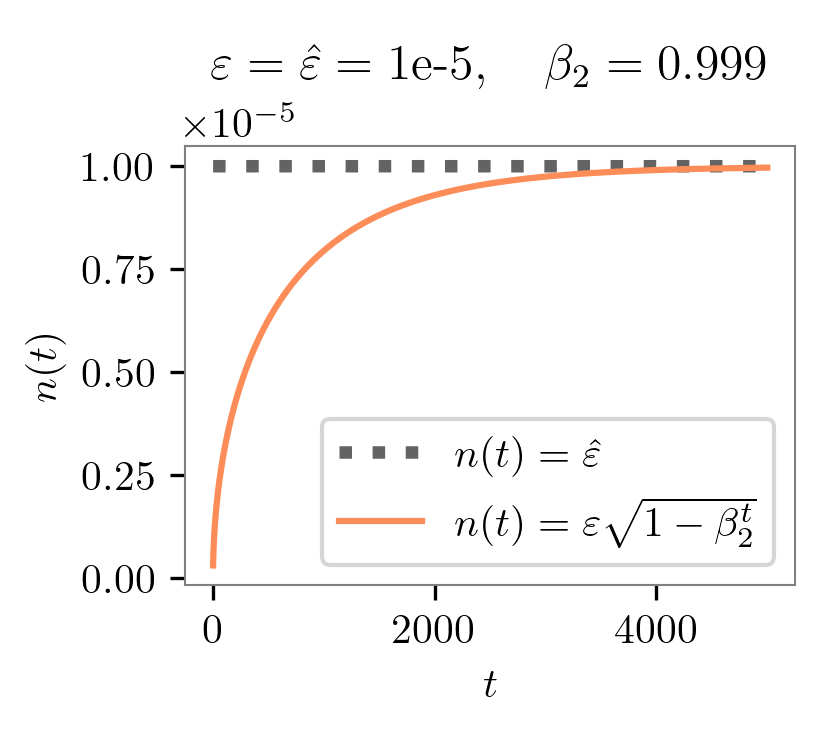 - The above figure shows that, if we set the same `eps` in pytorch adam and tensorflow adam, then pytorch-adam uses a much smaller normalization term than tensorflow-adam in the early phase of training. In other words, pytorch adam goes for **more aggressive gradient updates early in the training**. Our experiments support this finding, as we will demonstrate below. - How does this impact reproducibility and performance? To align settings, we record the original query, response, and rewards from [https://github.com/openai/lm-human-preferences](https://github.com/openai/lm-human-preferences) and save them in [https://huggingface.co/datasets/vwxyzjn/lm-human-preferences-debug/tree/main](https://huggingface.co/datasets/vwxyzjn/lm-human-preferences-debug/tree/main). I also record the metrics of the first two epochs of training with TF1’s `AdamOptimizer` optimizer as the ground truth. Below are some key metrics: | | OAI’s TF1 Adam | PyTorch’s Adam | Our custom Tensorflow-style Adam | | --- | --- | --- | --- | | policy/approxkl | 0.00037167023 | 0.0023672834504395723 | 0.000374998344341293 | | policy/clipfrac | 0.0045572915 | 0.02018229104578495 | 0.0052083334885537624 | | ratio_mean | 1.0051285 | 1.0105520486831665 | 1.0044583082199097 | | ratio_var | 0.0007716546 | 0.005374275613576174 | 0.0007942612282931805 | | ratio_max | 1.227216 | 1.8121057748794556 | 1.250215768814087 | | ratio_min | 0.7400441 | 0.4011387825012207 | 0.7299948930740356 | | logprob_diff_mean | 0.0047487603 | 0.008101251907646656 | 0.004073789343237877 | | logprob_diff_var | 0.0007207897 | 0.004668936599045992 | 0.0007334011606872082 | | logprob_diff_max | 0.20474821 | 0.594489574432373 | 0.22331619262695312 | | logprob_diff_min | -0.30104542 | -0.9134478569030762 | -0.31471776962280273 | - **PyTorch’s `Adam` produces a more aggressive update** for some reason. Here are some evidence: - **PyTorch’s `Adam`'s `logprob_diff_var`** **is 6x higher**. Here `logprobs_diff = new_logprobs - logprobs` is the difference between the log probability of tokens between the initial and current policy after two epochs of training. Having a larger `logprob_diff_var` means the scale of the log probability changes is larger than that in OAI’s TF1 Adam. - **PyTorch’s `Adam` presents a more extreme ratio max and min.** Here `ratio = torch.exp(logprobs_diff)`. Having a `ratio_max=1.8121057748794556` means that for some token, the probability of sampling that token is 1.8x more likely under the current policy, as opposed to only 1.2x with OAI’s TF1 Adam. - **Larger `policy/approxkl` `policy/clipfrac`.** Because of the aggressive update, the ratio gets clipped **4.4x more often, and the approximate KL divergence is 6x larger.** - The aggressive update is likely gonna cause further issues. E.g., `logprob_diff_mean` is 1.7x larger in PyTorch’s `Adam`, which would correspond to 1.7x larger KL penalty in the next reward calculation; this could get compounded. In fact, this might be related to the famous KL divergence issue — KL penalty is much larger than it should be and the model could pay more attention and optimizes for it more instead, therefore causing negative KL divergence. - **Larger models get affected more.** We conducted experiments comparing PyTorch’s `Adam` (codename `pt_adam`) and our custom TensorFlow-style (codename `tf_adam`) with `gpt2` and `gpt2-xl`. We found that the performance are roughly similar under `gpt2`; however with `gpt2-xl`, we observed a more aggressive updates, meaning that larger models get affected by this issue more. - When the initial policy updates are more aggressive in `gpt2-xl`, the training dynamics get affected. For example, we see a much larger `objective/kl` and `objective/scores` spikes with `pt_adam`, especially with `sentiment` — *the biggest KL was as large as 17.5* in one of the random seeds, suggesting an undesirable over-optimization. - Furthermore, because of the larger KL, many other training metrics are affected as well. For example, we see a much larger `clipfrac` (the fraction of time the `ratio` gets clipped by PPO’s objective clip coefficient 0.2) and `approxkl`. 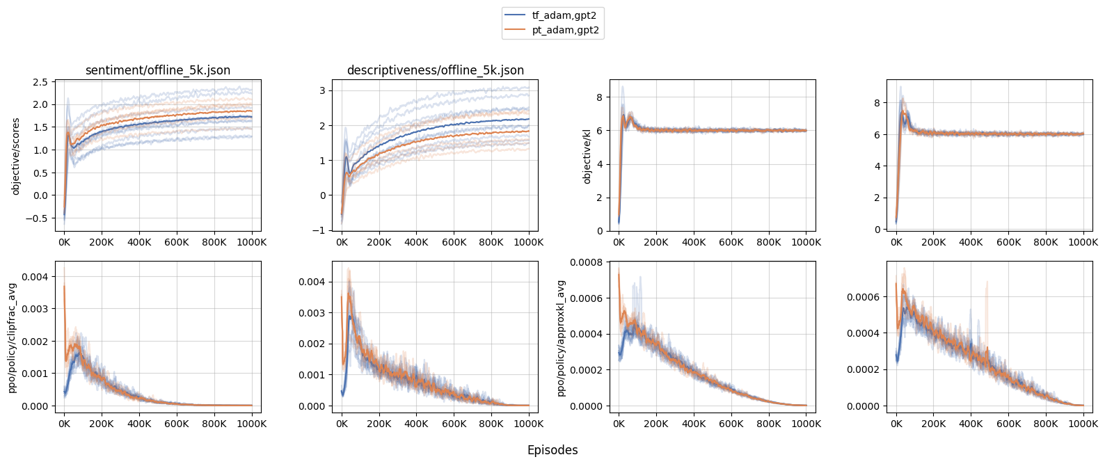 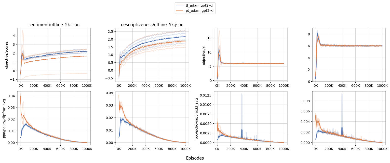 # Limitations Noticed this work does not try to reproduce the summarization work in CNN DM or TL;DR. This was because we found the training to be time-consuming and brittle. The particular training run we had showed poor GPU utilization (around 30%), so it takes almost 4 days to perform a training run, which is highly expensive (only AWS sells p3dn.24xlarge, and it costs $31.212 per hour) Additionally, training was brittle. While the reward goes up, we find it difficult to reproduce the “smart copier” behavior reported by Ziegler et al. (2019). Below are some sample outputs — clearly, the agent overfits somehow. See [https://wandb.ai/openrlbenchmark/lm-human-preferences/runs/1ab47rqi/logs](https://wandb.ai/openrlbenchmark/lm-human-preferences/runs/1ab47rqi/logs?workspace=user-costa-huang) for more complete logs. 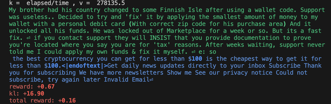 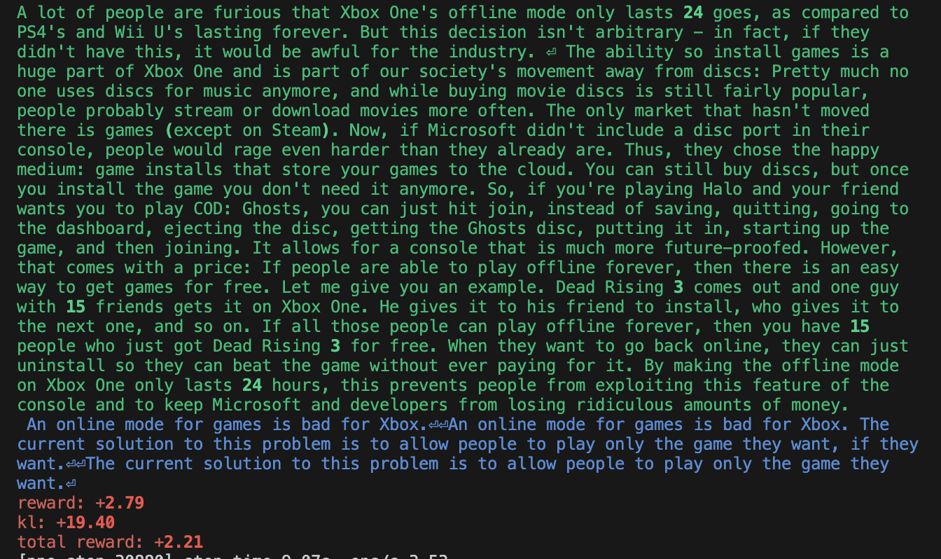 # Conclusion In this work, we took a deep dive into OAI’s original RLHF codebase and compiled a list of its implementation details. We also created a minimal base which reproduces the same learning curves as OAI’s original RLHF codebase, when the dataset and hyperparameters are controlled. Furthermore, we identify surprising implementation details such as the adam optimizer’s setting which causes aggressive updates in early RLHF training. # Acknowledgement This work is supported by Hugging Face’s Big Science cluster 🤗. We also thank the helpful discussion with @lewtun and @natolambert. # Bibtex ```bibtex @article{Huang2023implementation, author = {Huang, Shengyi and Liu, Tianlin and von Werra, Leandro}, title = {The N Implementation Details of RLHF with PPO}, journal = {Hugging Face Blog}, year = {2023}, note = {https://huggingface.co/blog/the_n_implementation_details_of_rlhf_with_ppo}, } ```"
Deploy Embedding Models with Hugging Face Inference Endpoints,philschmid,"October 24, 2023",inference-endpoints-embeddings,"guide, llm, apps, inference",https://huggingface.co/blog/inference-endpoints-embeddings," # Deploy Embedding Models with Hugging Face Inference Endpoints The rise of Generative AI and LLMs like ChatGPT has increased the interest and importance of embedding models for a variety of tasks especially for retrievel augemented generation, like search or chat with your data. Embeddings are helpful since they represent sentences, images, words, etc. as numeric vector representations, which allows us to map semantically related items and retrieve helpful information. This helps us to provide relevant context for our prompt to improve the quality and specificity of generation. Compared to LLMs are Embedding Models smaller in size and faster for inference. That is very important since you need to recreate your embeddings after you changed your model or improved your model fine-tuning. Additionally, is it important that the whole retrieval augmentation process is as fast as possible to provide a good user experience. In this blog post, we will show you how to deploy open-source Embedding Models to [Hugging Face Inference Endpoints](https://ui.endpoints.huggingface.co/) using [Text Embedding Inference](https://github.com/huggingface/text-embeddings-inference), our managed SaaS solution that makes it easy to deploy models. Additionally, we will teach you how to run large scale batch requests. 1. [What is Hugging Face Inference Endpoints](#1-what-is-hugging-face-inference-endpoints) 2. [What is Text Embedding Inference](#2-what-is-text-embeddings-inference) 3. [Deploy Embedding Model as Inference Endpoint](#3-deploy-embedding-model-as-inference-endpoint) 4. [Send request to endpoint and create embeddings](#4-send-request-to-endpoint-and-create-embeddings) Before we start, let's refresh our knowledge about Inference Endpoints. ## 1. What is Hugging Face Inference Endpoints? [Hugging Face Inference Endpoints](https://ui.endpoints.huggingface.co/) offers an easy and secure way to deploy Machine Learning models for use in production. Inference Endpoints empower developers and data scientists to create Generative AI applications without managing infrastructure: simplifying the deployment process to a few clicks, including handling large volumes of requests with autoscaling, reducing infrastructure costs with scale-to-zero, and offering advanced security. Here are some of the most important features: 1. [Easy Deployment](https://huggingface.co/docs/inference-endpoints/index): Deploy models as production-ready APIs with just a few clicks, eliminating the need to handle infrastructure or MLOps. 2. [Cost Efficiency](https://huggingface.co/docs/inference-endpoints/autoscaling): Benefit from automatic scale to zero capability, reducing costs by scaling down the infrastructure when the endpoint is not in use, while paying based on the uptime of the endpoint, ensuring cost-effectiveness. 3. [Enterprise Security](https://huggingface.co/docs/inference-endpoints/security): Deploy models in secure offline endpoints accessible only through direct VPC connections, backed by SOC2 Type 2 certification, and offering BAA and GDPR data processing agreements for enhanced data security and compliance. 4. [LLM Optimization](https://huggingface.co/text-generation-inference): Optimized for LLMs, enabling high throughput with Paged Attention and low latency through custom transformers code and Flash Attention power by Text Generation Inference 5. [Comprehensive Task Support](https://huggingface.co/docs/inference-endpoints/supported_tasks): Out of the box support for 🤗 Transformers, Sentence-Transformers, and Diffusers tasks and models, and easy customization to enable advanced tasks like speaker diarization or any Machine Learning task and library. You can get started with Inference Endpoints at: https://ui.endpoints.huggingface.co/ ## 2. What is Text Embeddings Inference? [Text Embeddings Inference (TEI)](https://github.com/huggingface/text-embeddings-inference#text-embeddings-inference) is a purpose built solution for deploying and serving open source text embeddings models. TEI is build for high-performance extraction supporting the most popular models. TEI supports all top 10 models of the [Massive Text Embedding Benchmark (MTEB) Leaderboard](https://huggingface.co/spaces/mteb/leaderboard), including FlagEmbedding, Ember, GTE and E5. TEI currently implements the following performance optimizing features: - No model graph compilation step - Small docker images and fast boot times. Get ready for true serverless! - Token based dynamic batching - Optimized transformers code for inference using [Flash Attention](https://github.com/HazyResearch/flash-attention), [Candle](https://github.com/huggingface/candle) and [cuBLASLt](https://docs.nvidia.com/cuda/cublas/#using-the-cublaslt-api) - [Safetensors](https://github.com/huggingface/safetensors) weight loading - Production ready (distributed tracing with Open Telemetry, Prometheus metrics) Those feature enabled industry-leading performance on throughput and cost. In a benchmark for [BAAI/bge-base-en-v1.5](https://huggingface.co/BAAI/bge-base-en-v1.5) on an Nvidia A10G Inference Endpoint with a sequence length of 512 tokens and a batch size of 32, we achieved a throughput of 450+ req/sec resulting into a cost of 0.00156$ / 1M tokens or 0.00000156$ / 1k tokens. That is 64x cheaper than OpenAI Embeddings ($0.0001 / 1K tokens). 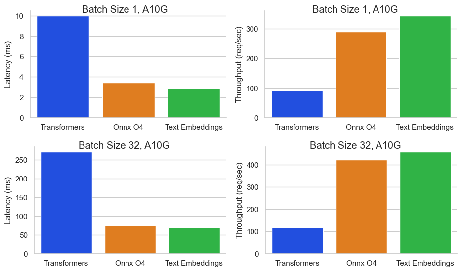 ## 3. Deploy Embedding Model as Inference Endpoint To get started, you need to be logged in with a User or Organization account with a payment method on file (you can add one [here](https://huggingface.co/settings/billing)), then access Inference Endpoints at [https://ui.endpoints.huggingface.co](https://ui.endpoints.huggingface.co/endpoints) Then, click on “New endpoint”. Select the repository, the cloud, and the region, adjust the instance and security settings, and deploy in our case `BAAI/bge-base-en-v1.5`. 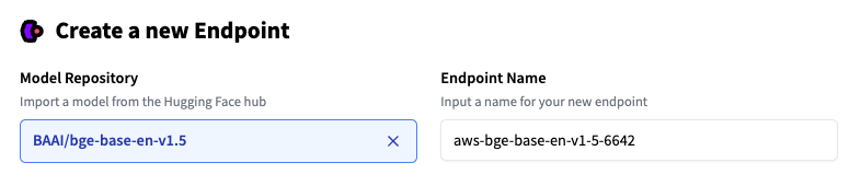 Inference Endpoints suggest an instance type based on the model size, which should be big enough to run the model. Here `Intel Ice Lake 2 vCPU`. To get the performance for the benchmark we ran you, change the instance to `1x Nvidia A10G`. *Note: If the instance type cannot be selected, you need to [contact us](mailto:api-enterprise@huggingface.co?subject=Quota%20increase%20HF%20Endpoints&body=Hello,%0D%0A%0D%0AI%20would%20like%20to%20request%20access/quota%20increase%20for%20%7BINSTANCE%20TYPE%7D%20for%20the%20following%20account%20%7BHF%20ACCOUNT%7D.) and request an instance quota.* 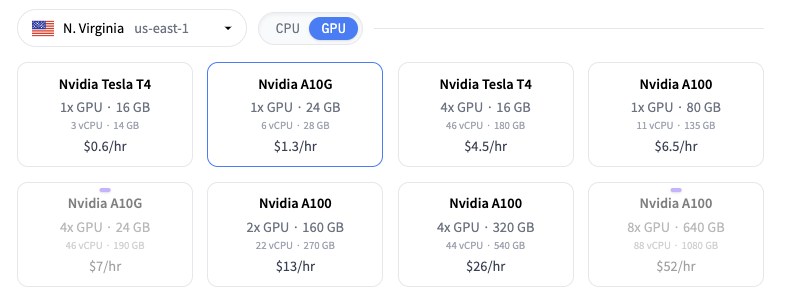 You can then deploy your model with a click on “Create Endpoint”. After 1-3 minutes, the Endpoint should be online and available to serve requests. ## 4. Send request to endpoint and create embeddings The Endpoint overview provides access to the Inference Widget, which can be used to manually send requests. This allows you to quickly test your Endpoint with different inputs and share it with team members. 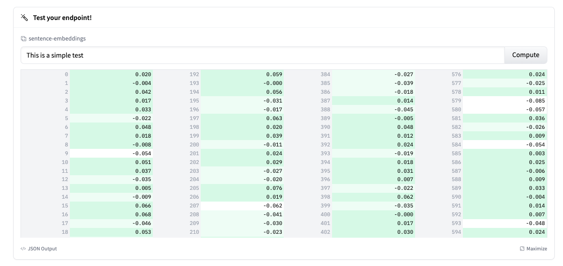 *Note: TEI is currently is not automatically truncating the input. You can enable this by setting `truncate: true` in your request.* In addition to the widget the overview provides an code snippet for cURL, Python and Javascript, which you can use to send request to the model. The code snippet shows you how to send a single request, but TEI also supports batch requests, which allows you to send multiple document at the same to increase utilization of your endpoint. Below is an example on how to send a batch request with truncation set to true. ```python import requests API_URL = ""https://l2skjfwp9punv393.us-east-1.aws.endpoints.huggingface.cloud"" headers = { ""Authorization"": ""Bearer YOUR TOKEN"", ""Content-Type"": ""application/json"" } def query(payload): response = requests.post(API_URL, headers=headers, json=payload) return response.json() output = query({ ""inputs"": [""sentence 1"", ""sentence 2"", ""sentence 3""], ""truncate"": True }) # output [[0.334, ...], [-0.234, ...]] ``` ## Conclusion TEI on Hugging Face Inference Endpoints enables blazing fast and ultra cost-efficient deployment of state-of-the-art embeddings models. With industry-leading throughput of 450+ requests per second and costs as low as $0.00000156 / 1k tokens, Inference Endpoints delivers 64x cost savings compared to OpenAI Embeddings. For developers and companies leveraging text embeddings to enable semantic search, chatbots, recommendations, and more, Hugging Face Inference Endpoints eliminates infrastructure overhead and delivers high throughput at lowest cost streamlining the process from research to production. --- Thanks for reading! If you have any questions, feel free to contact me on [Twitter](https://twitter.com/_philschmid) or [LinkedIn](https://www.linkedin.com/in/philipp-schmid-a6a2bb196/)."
Interactively explore your Huggingface dataset with one line of code,sps44,"October 25, 2023",scalable-data-inspection,"open-source-collab, visualization, data inspection",https://huggingface.co/blog/scalable-data-inspection," # Interactively explore your Huggingface dataset with one line of code The Hugging Face [*datasets* library](https://huggingface.co/docs/datasets/index) not only provides access to more than 70k publicly available datasets, but also offers very convenient data preparation pipelines for custom datasets. [Renumics Spotlight](https://github.com/Renumics/spotlight) allows you to create **interactive visualizations** to **identify critical clusters** in your data. Because Spotlight understands the data semantics within Hugging Face datasets, you can **[get started with just one line of code](https://renumics.com/docs)**: ```python import datasets from renumics import spotlight ds = datasets.load_dataset('speech_commands', 'v0.01', split='validation') spotlight.show(ds) ``` ![]()
Spotlight allows to **leverage model results** such as predictions and embeddings to gain a deeper understanding in data segments and model failure modes: ```python ds_results = datasets.load_dataset('renumics/speech_commands-ast-finetuned-results', 'v0.01', split='validation') ds = datasets.concatenate_datasets([ds, ds_results], axis=1) spotlight.show(ds, dtype={'embedding': spotlight.Embedding}, layout=spotlight.layouts.debug_classification(embedding='embedding', inspect={'audio': spotlight.dtypes.audio_dtype})) ``` Data inspection is a very important task in almost all ML development stages, but it can also be very time consuming. > “Manual inspection of data has probably the highest value-to-prestige ratio of any activity in machine learning.” — Greg Brockman > [Spotlight](https://renumics.com/docs) helps you to **make data inspection more scalable** along two dimensions: Setting up and maintaining custom data inspection workflows and finding relevant data samples and clusters to inspect. In the following sections we show some examples based on Hugging Face datasets. ## Spotlight 🤝 Hugging Face datasets The *datasets* library has several features that makes it an ideal tool for working with ML datasets: It stores tabular data (e.g. metadata, labels) along with unstructured data (e.g. images, audio) in a common Arrows table. *Datasets* also describes important data semantics through features (e.g. images, audio) and additional task-specific metadata. Spotlight directly works on top of the *datasets* library. This means that there is no need to copy or pre-process the dataset for data visualization and inspection. Spotlight loads the tabular data into memory to allow for efficient, client-side data analytics. Memory-intensive unstructured data samples (e.g. audio, images, video) are loaded lazily on demand. In most cases, data types and label mappings are inferred directly from the dataset. Here, we visualize the CIFAR-100 dataset with one line of code: ```python ds = datasets.load_dataset('cifar100', split='test') spotlight.show(ds) ``` In cases where the data types are ambiguous or not specified, the Spotlight API allows to manually assign them: ```python label_mapping = dict(zip(ds.features['fine_label'].names, range(len(ds.features['fine_label'].names)))) spotlight.show(ds, dtype={'img': spotlight.Image, 'fine_label': spotlight.dtypes.CategoryDType(categories=label_mapping)}) ``` ## **Leveraging model results for data inspection** Exploring raw unstructured datasets often yield little insights. Leveraging model results such as predictions or embeddings can help to uncover critical data samples and clusters. Spotlight has several visualization options (e.g. similarity map, confusion matrix) that specifically make use of model results. We recommend storing your prediction results directly in a Hugging Face dataset. This not only allows you to take advantage of the batch processing capabilities of the datasets library, but also keeps label mappings. We can use the [*transformers* library](https://huggingface.co/docs/transformers) to compute embeddings and predictions on the CIFAR-100 image classification problem. We install the libraries via pip: ```bash pip install renumics-spotlight datasets transformers[torch] ``` Now we can compute the enrichment: ```python import torch import transformers device = torch.device(""cuda:0"" if torch.cuda.is_available() else ""cpu"") model_name = ""Ahmed9275/Vit-Cifar100"" processor = transformers.ViTImageProcessor.from_pretrained(model_name) cls_model = transformers.ViTForImageClassification.from_pretrained(model_name).to(device) fe_model = transformers.ViTModel.from_pretrained(model_name).to(device) def infer(batch): images = [image.convert(""RGB"") for image in batch] inputs = processor(images=images, return_tensors=""pt"").to(device) with torch.no_grad(): outputs = cls_model(**inputs) probs = torch.nn.functional.softmax(outputs.logits, dim=-1).cpu().numpy() embeddings = fe_model(**inputs).last_hidden_state[:, 0].cpu().numpy() preds = probs.argmax(axis=-1) return {""prediction"": preds, ""embedding"": embeddings} features = datasets.Features({**ds.features, ""prediction"": ds.features[""fine_label""], ""embedding"": datasets.Sequence(feature=datasets.Value(""float32""), length=768)}) ds_enriched = ds.map(infer, input_columns=""img"", batched=True, batch_size=2, features=features) ``` If you don’t want to perform the full inference run, you can alternatively download pre-computed model results for CIFAR-100 to follow this tutorial: ```python ds_results = datasets.load_dataset('renumics/spotlight-cifar100-enrichment', split='test') ds_enriched = datasets.concatenate_datasets([ds, ds_results], axis=1) ``` We can now use the results to interactively explore relevant data samples and clusters in Spotlight: ```python layout = spotlight.layouts.debug_classification(label='fine_label', embedding='embedding', inspect={'img': spotlight.dtypes.image_dtype}) spotlight.show(ds_enriched, dtype={'embedding': spotlight.Embedding}, layout=layout) ``` ![]() ## Customizing data inspection workflows Visualization layouts can be interactively changed, saved and loaded in the GUI: You can select different widget types and configurations. The *Inspector* widget allows to represent multimodal data samples including text, image, audio, video and time series data. You can also define layouts through the [Python API](https://renumics.com/api/spotlight/). This option is especially useful for building custom data inspection and curation workflows including EDA, model debugging and model monitoring tasks. In combination with the data issues widget, the Python API offers a great way to integrate the results of existing scripts (e.g. data quality checks or model monitoring) into a scalable data inspection workflow. ## Using Spotlight on the Hugging Face hub You can use Spotlight directly on your local NLP, audio, CV or multimodal dataset. If you would like to showcase your dataset or model results on the Hugging Face hub, you can use Hugging Face spaces to launch a Spotlight visualization for it. We have already prepared [example spaces](https://huggingface.co/renumics) for many popular NLP, audio and CV datasets on the hub. You can simply duplicate one of these spaces and specify your dataset in the `HF_DATASET` variable. You can optionally choose a dataset that contains model results and other configuration options such as splits, subsets or dataset revisions.
## Customizing data inspection workflows Visualization layouts can be interactively changed, saved and loaded in the GUI: You can select different widget types and configurations. The *Inspector* widget allows to represent multimodal data samples including text, image, audio, video and time series data. You can also define layouts through the [Python API](https://renumics.com/api/spotlight/). This option is especially useful for building custom data inspection and curation workflows including EDA, model debugging and model monitoring tasks. In combination with the data issues widget, the Python API offers a great way to integrate the results of existing scripts (e.g. data quality checks or model monitoring) into a scalable data inspection workflow. ## Using Spotlight on the Hugging Face hub You can use Spotlight directly on your local NLP, audio, CV or multimodal dataset. If you would like to showcase your dataset or model results on the Hugging Face hub, you can use Hugging Face spaces to launch a Spotlight visualization for it. We have already prepared [example spaces](https://huggingface.co/renumics) for many popular NLP, audio and CV datasets on the hub. You can simply duplicate one of these spaces and specify your dataset in the `HF_DATASET` variable. You can optionally choose a dataset that contains model results and other configuration options such as splits, subsets or dataset revisions. ![]() ## What’s next? With Spotlight you can create **interactive visualizations** and leverage data enrichments to **identify critical clusters** in your Hugging Face datasets. In this blog, we have seen both an audio ML and a computer vision example. You can use Spotlight directly to explore and curate your NLP, audio, CV or multimodal dataset: - Install Spotlight: *pip install renumics-spotlight* - Check out the [documentation](https://renumics.com/docs) or open an issue on [Github](https://github.com/Renumics/spotlight) - Join the [Spotlight community](https://discord.gg/VAQdFCU5YD) on Discord - Follow us on [Twitter](https://twitter.com/renumics) and [LinkedIn](https://www.linkedin.com/company/renumics)"
Personal Copilot: Train Your Own Coding Assistant,smangrul,"October 27, 2023",personal-copilot,"bigcode, llm, nlp, inference, guide",https://huggingface.co/blog/personal-copilot," # Personal Copilot: Train Your Own Coding Assistant In the ever-evolving landscape of programming and software development, the quest for efficiency and productivity has led to remarkable innovations. One such innovation is the emergence of code generation models such as [Codex](https://openai.com/blog/openai-codex), [StarCoder](https://arxiv.org/abs/2305.06161) and [Code Llama](https://arxiv.org/abs/2308.12950). These models have demonstrated remarkable capabilities in generating human-like code snippets, thereby showing immense potential as coding assistants. However, while these pre-trained models can perform impressively across a range of tasks, there's an exciting possibility lying just beyond the horizon: the ability to tailor a code generation model to your specific needs. Think of personalized coding assistants which could be leveraged at an enterprise scale. In this blog post we show how we created HugCoder 🤗, a code LLM fine-tuned on the code contents from the public repositories of the [`huggingface` GitHub organization](https://github.com/huggingface). We will discuss our data collection workflow, our training experiments, and some interesting results. This will enable you to create your own personal copilot based on your proprietary codebase. We will leave you with a couple of further extensions of this project for experimentation. Let’s begin 🚀  ## Data Collection Workflow Our desired dataset is conceptually simple, we structured it like so: | | | | |---|---|---| | Repository Name | Filepath in the Repository | File Contents | |---|---|---| |---|---|---| Scraping code contents from GitHub is straightforward with the [Python GitHub API](https://github.com/PyGithub/PyGithub). However, depending on the number of repositories and the number of code files within a repository, one might easily run into API rate-limiting issues. To prevent such problems, we decided to clone all the public repositories locally and extract the contents from them instead of through the API. We used the `multiprocessing` module from Python to download all repos in parallel, as shown in [this download script](https://github.com/sayakpaul/hf-codegen/blob/main/data/parallel_clone_repos.py). A repository can often contain non-code files such as images, presentations and other assets. We’re not interested in scraping them. We created a [list of extensions](https://github.com/sayakpaul/hf-codegen/blob/f659eba76f07e622873211e5b975168b634e6c22/data/prepare_dataset.py#L17C1-L49C68) to filter them out. To parse code files other than Jupyter Notebooks, we simply used the ""utf-8"" encoding. For notebooks, we only considered the code cells. We also excluded all file paths that were not directly related to code. These include: `.git`, `__pycache__`, and `xcodeproj`. To keep the serialization of this content relatively memory-friendly, we used chunking and the [feather format](https://arrow.apache.org/docs/python/feather.html#:~:text=Feather%20is%20a%20portable%20file,Python%20(pandas)%20and%20R.). Refer to [this script](https://github.com/sayakpaul/hf-codegen/blob/main/data/prepare_dataset.py) for the full implementation. The final dataset is [available on the Hub](https://huggingface.co/datasets/sayakpaul/hf-codegen-v2), and it looks like this: 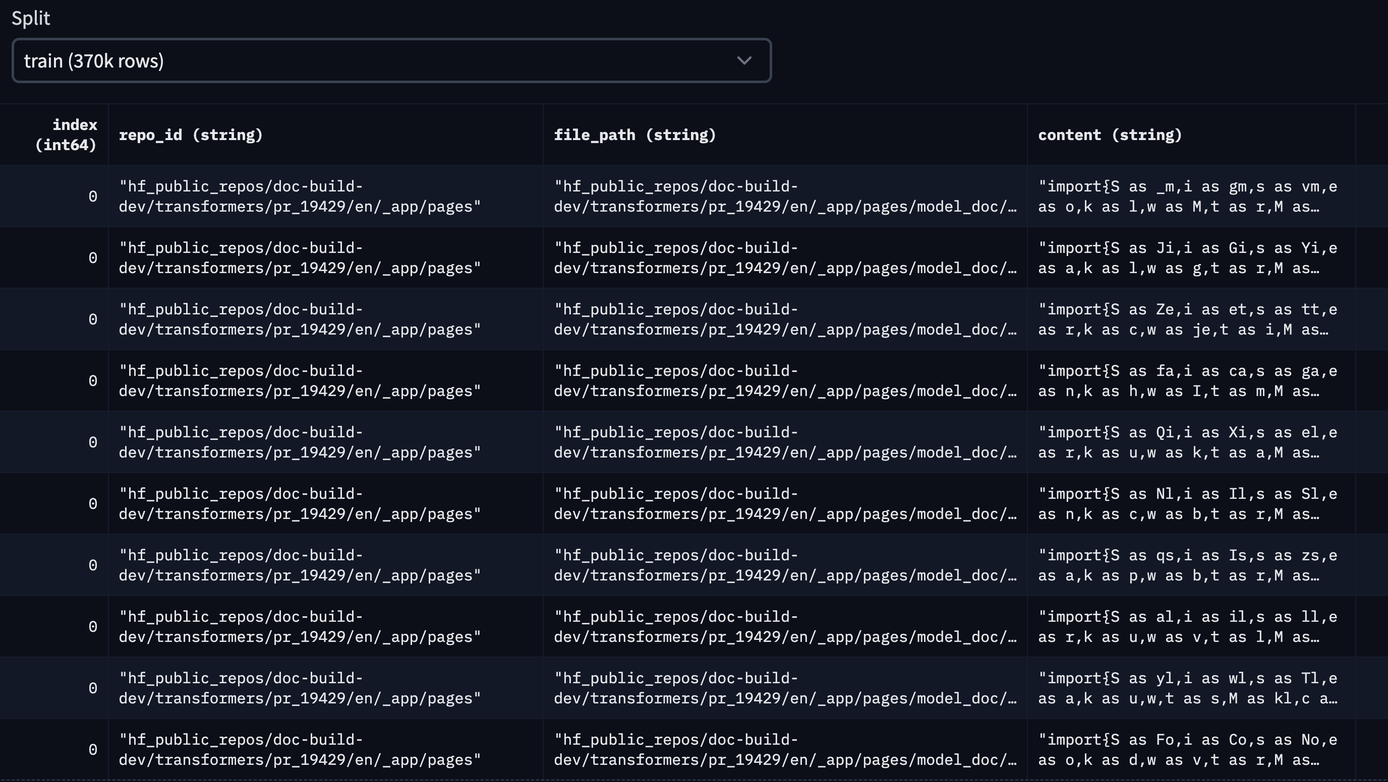 For this blog, we considered the top 10 Hugging Face public repositories, based on stargazers. They are the following: > ['transformers', 'pytorch-image-models', 'datasets', 'diffusers', 'peft', 'tokenizers', 'accelerate', 'text-generation-inference', 'chat-ui', 'deep-rl-class'] [This is the code we used to generate this dataset](https://github.com/pacman100/DHS-LLM-Workshop/tree/main/personal_copilot/dataset_generation), and [this is the dataset in the Hub](https://huggingface.co/datasets/smangrul/hf-stack-v1). Here is a snapshot of what it looks like: 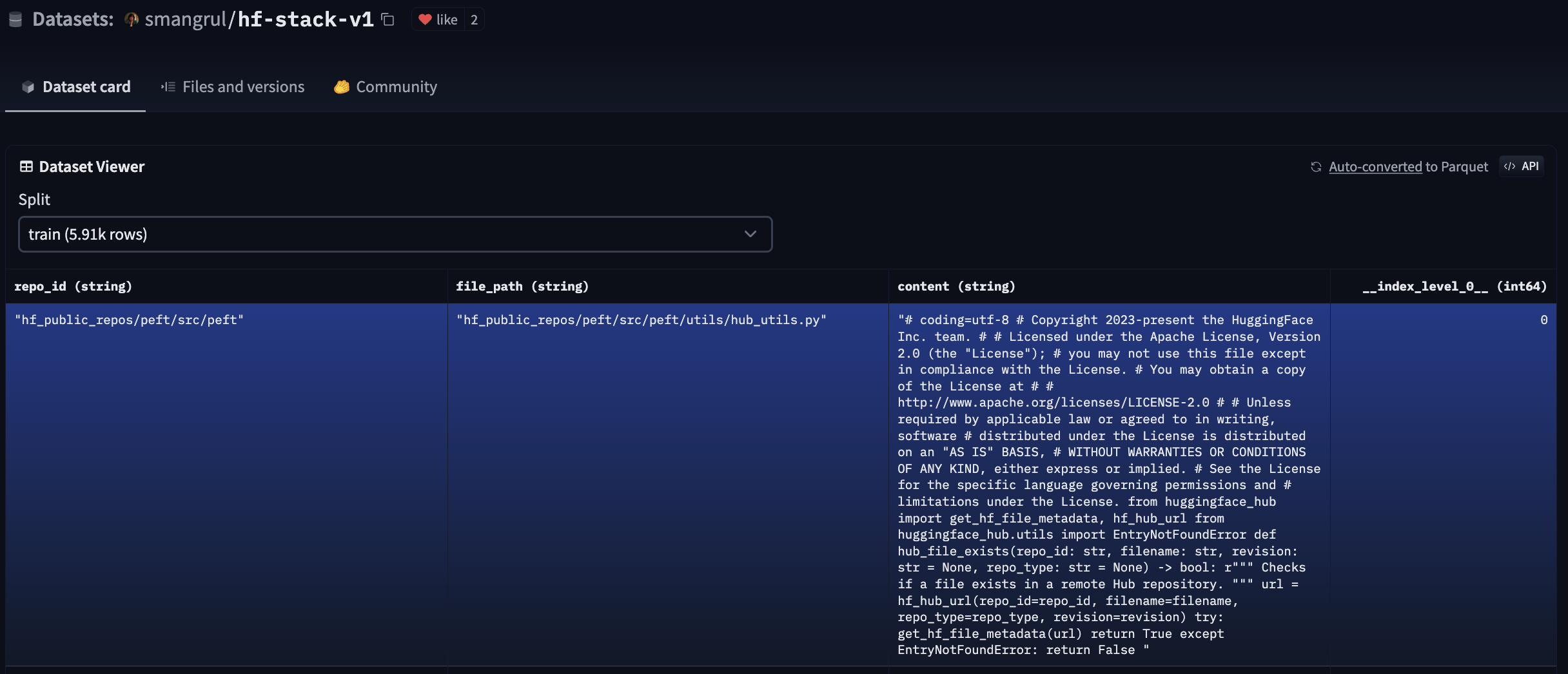 To reduce the project complexity, we didn’t consider deduplication of the dataset. If you are interested in applying deduplication techniques for a production application, [this blog post](https://huggingface.co/blog/dedup) is an excellent resource about the topic in the context of code LLMs. ## Finetuning your own Personal Co-Pilot In this section, we show how to fine-tune the following models: [`bigcode/starcoder`](https://hf.co/bigcode/starcoder) (15.5B params), [`bigcode/starcoderbase-1b`](https://hf.co/bigcode/starcoderbase-1b) (1B params), [`Deci/DeciCoder-1b`](https://hf.co/Deci/DeciCoder-1b) (1B params). We'll use a single A100 40GB Colab Notebook using 🤗 PEFT (Parameter-Efficient Fine-Tuning) for all the experiments. Additionally, we'll show how to fully finetune the `bigcode/starcoder` (15.5B params) on a machine with 8 A100 80GB GPUs using 🤗 Accelerate's FSDP integration. The training objective is [fill in the middle (FIM)](https://arxiv.org/abs/2207.14255), wherein parts of a training sequence are moved to the end, and the reordered sequence is predicted auto-regressively. Why PEFT? Full fine-tuning is expensive. Let’s have some numbers to put things in perspective: Minimum GPU memory required for full fine-tuning: 1. Weight: 2 bytes (Mixed-Precision training) 2. Weight gradient: 2 bytes 3. Optimizer state when using Adam: 4 bytes for original FP32 weight + 8 bytes for first and second moment estimates 4. Cost per parameter adding all of the above: 16 bytes per parameter 5. **15.5B model -> 248GB of GPU memory without even considering huge memory requirements for storing intermediate activations -> minimum 4X A100 80GB GPUs required** Since the hardware requirements are huge, we'll be using parameter-efficient fine-tuning using [QLoRA](https://arxiv.org/abs/2305.14314). Here are the minimal GPU memory requirements for fine-tuning StarCoder using QLoRA: > trainable params: 110,428,160 || all params: 15,627,884,544 || trainable%: 0.7066097761926236 1. Base model Weight: 0.5 bytes * 15.51B frozen params = 7.755 GB 2. Adapter weight: 2 bytes * 0.11B trainable params = 0.22GB 3. Weight gradient: 2 bytes * 0.11B trainable params = 0.12GB 4. Optimizer state when using Adam: 4 bytes * 0.11B trainable params * 3 = 1.32GB 5. **Adding all of the above -> 9.51 GB ~10GB -> 1 A100 40GB GPU required** 🤯. The reason for A100 40GB GPU is that the intermediate activations for long sequence lengths of 2048 and batch size of 4 for training lead to higher memory requirements. As we will see below, GPU memory required is 26GB which can be accommodated on A100 40GB GPU. Also, A100 GPUs have better compatibilty with Flash Attention 2. In the above calculations, we didn't consider memory required for intermediate activation checkpointing which is considerably huge. We leverage Flash Attention V2 and Gradient Checkpointing to overcome this issue. 1. For QLoRA along with flash attention V2 and gradient checkpointing, the total memory occupied by the model on a single A100 40GB GPU is **26 GB** with a **batch size of 4**. 2. For full fine-tuning using FSDP along with Flash Attention V2 and Gradient Checkpointing, the memory occupied per GPU ranges between **70 GB to 77.6 GB** with a **per_gpu_batch_size of 1**. Please refer to the [model-memory-usage](https://huggingface.co/spaces/hf-accelerate/model-memory-usage) to easily calculate how much vRAM is needed to train and perform big model inference on a model hosted on the 🤗 Hugging Face Hub. ## Full Finetuning We will look at how to do full fine-tuning of `bigcode/starcoder` (15B params) on 8 A100 80GB GPUs using PyTorch Fully Sharded Data Parallel (FSDP) technique. For more information on FSDP, please refer to [Fine-tuning Llama 2 70B using PyTorch FSDP](https://huggingface.co/blog/ram-efficient-pytorch-fsdp) and [Accelerate Large Model Training using PyTorch Fully Sharded Data Parallel](https://huggingface.co/blog/pytorch-fsdp). **Resources** 1. Codebase: [link](https://github.com/pacman100/DHS-LLM-Workshop/tree/main/personal_copilot/training). It uses the recently added Flash Attention V2 support in Transformers. 2. FSDP Config: [fsdp_config.yaml](https://github.com/pacman100/DHS-LLM-Workshop/blob/main/personal_copilot/training/configs/fsdp_config.yaml) 3. Model: [bigcode/stacoder](https://huggingface.co/bigcode/starcoder) 4. Dataset: [smangrul/hf-stack-v1](https://huggingface.co/datasets/smangrul/hf-stack-v1) 5. Fine-tuned Model: [smangrul/peft-lora-starcoder15B-v2-personal-copilot-A100-40GB-colab](https://huggingface.co/smangrul/peft-lora-starcoder15B-v2-personal-copilot-A100-40GB-colab) The command to launch training is given at [run_fsdp.sh](https://github.com/pacman100/DHS-LLM-Workshop/blob/main/personal_copilot/training/run_fsdp.sh). ``` accelerate launch --config_file ""configs/fsdp_config.yaml"" train.py \ --model_path ""bigcode/starcoder"" \ --dataset_name ""smangrul/hf-stack-v1"" \ --subset ""data"" \ --data_column ""content"" \ --split ""train"" \ --seq_length 2048 \ --max_steps 2000 \ --batch_size 1 \ --gradient_accumulation_steps 2 \ --learning_rate 5e-5 \ --lr_scheduler_type ""cosine"" \ --weight_decay 0.01 \ --num_warmup_steps 30 \ --eval_freq 100 \ --save_freq 500 \ --log_freq 25 \ --num_workers 4 \ --bf16 \ --no_fp16 \ --output_dir ""starcoder-personal-copilot-A100-40GB-colab"" \ --fim_rate 0.5 \ --fim_spm_rate 0.5 \ --use_flash_attn ``` The total training time was **9 Hours**. Taking the cost of $12.00 / hr based on [lambdalabs](https://lambdalabs.com/service/gpu-cloud/pricing) for 8x A100 80GB GPUs, the total cost would be **$108**. ## PEFT We will look at how to use QLoRA for fine-tuning `bigcode/starcoder` (15B params) on a single A100 40GB GPU using 🤗 PEFT. For more information on QLoRA and PEFT methods, please refer to [Making LLMs even more accessible with bitsandbytes, 4-bit quantization and QLoRA](https://huggingface.co/blog/4bit-transformers-bitsandbytes) and [🤗 PEFT: Parameter-Efficient Fine-Tuning of Billion-Scale Models on Low-Resource Hardware](https://huggingface.co/blog/peft). **Resources** 1. Codebase: [link](https://github.com/pacman100/DHS-LLM-Workshop/tree/main/personal_copilot/training). It uses the recently added Flash Attention V2 support in Transformers. 2. Colab notebook: [link](https://colab.research.google.com/drive/1Tz9KKgacppA4S6H4eo_sw43qEaC9lFLs?usp=sharing). Make sure to choose A100 GPU with High RAM setting. 3. Model: [bigcode/stacoder](https://huggingface.co/bigcode/starcoder) 4. Dataset: [smangrul/hf-stack-v1](https://huggingface.co/datasets/smangrul/hf-stack-v1) 5. QLoRA Fine-tuned Model: [smangrul/peft-lora-starcoder15B-v2-personal-copilot-A100-40GB-colab](https://huggingface.co/smangrul/peft-lora-starcoder15B-v2-personal-copilot-A100-40GB-colab) The command to launch training is given at [run_peft.sh](https://github.com/pacman100/DHS-LLM-Workshop/blob/main/personal_copilot/training/run_peft.sh). The total training time was **12.5 Hours**. Taking the cost of **$1.10 / hr** based on [lambdalabs](https://lambdalabs.com/service/gpu-cloud/pricing), the total cost would be **$13.75**. That's pretty good 🚀! In terms of cost, it's **7.8X** lower than the cost for full fine-tuning. ## Comparison The plot below shows the eval loss, train loss and learning rate scheduler for QLoRA vs full fine-tuning. We observe that full fine-tuning leads to slightly lower loss and converges a bit faster compared to QLoRA. The learning rate for peft fine-tuning is 10X more than that of full fine-tuning. 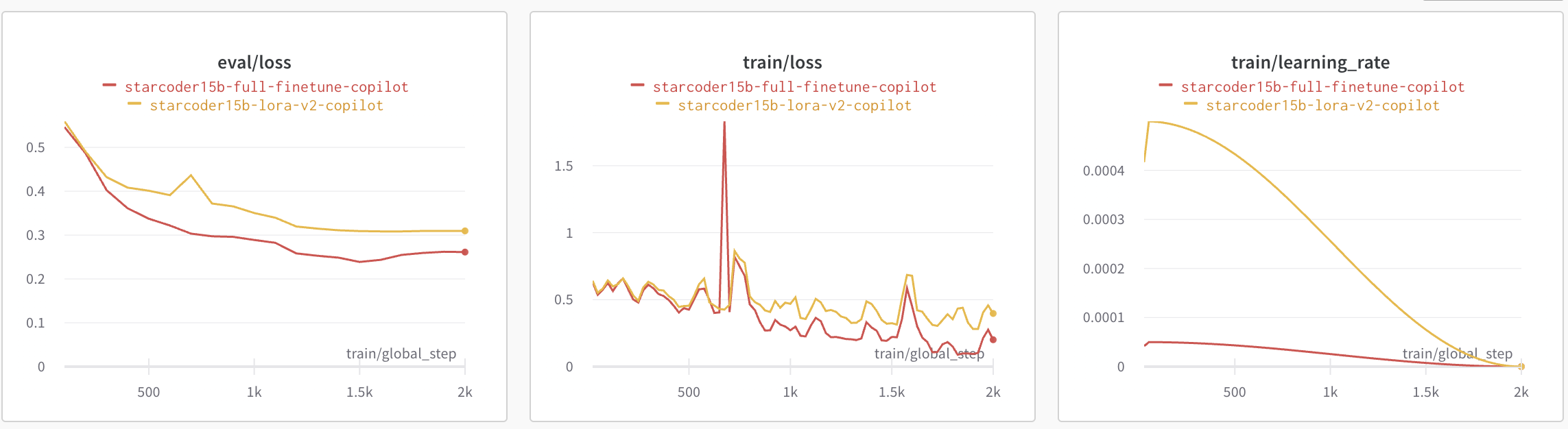 To make sure that our QLoRA model doesn't lead to catastrophic forgetting, we run the Python Human Eval on it. Below are the results we got. `Pass@1` measures the pass rate of completions considering just a single generated code candidate per problem. We can observe that the performance on `humaneval-python` is comparable between the base `bigcode/starcoder` (15B params) and the fine-tuned PEFT model `smangrul/peft-lora-starcoder15B-v2-personal-copilot-A100-40GB-colab`. | | | |---|---| | Model | Pass@1 | |bigcode/starcoder | 33.57| |smangrul/peft-lora-starcoder15B-v2-personal-copilot-A100-40GB-colab| 33.37 | Let's now look at some qualitative samples. In our manual analysis, we noticed that the QLoRA led to slight overfitting and as such we down weigh it by creating new weighted adapter with weight 0.8 via `add_weighted_adapter` utility of PEFT. We will look at 2 code infilling examples wherein the task of the model is to fill the part denoted by the `` placeholder. We will consider infilling completions from GitHub Copilot, the QLoRA fine-tuned model and the full fine-tuned model. 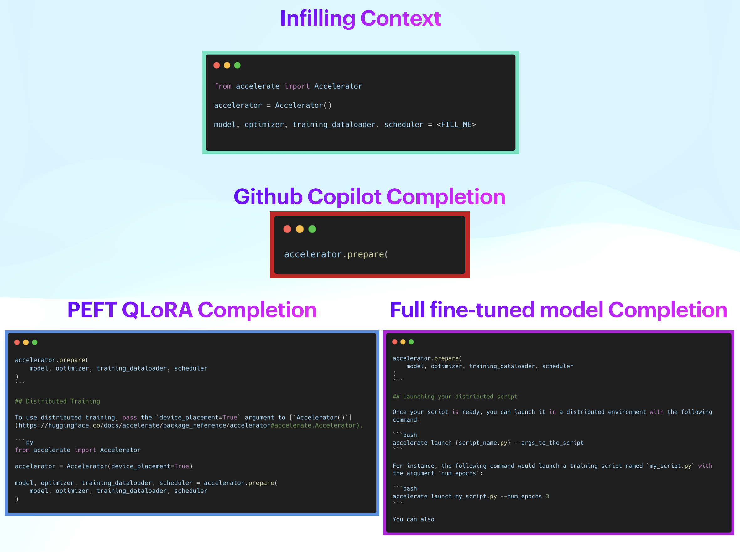 *Qualitative Example 1* In the example above, the completion from GitHub Copilot is along the correct lines but doesn't help much. On the other hand, completions from QLoRA and full fine-tuned models are correctly infilling the entire function call with the necessary parameters. However, they are also adding a lot more noise afterwards. This could be controlled with a post-processing step to limit completions to closing brackets or new lines. Note that both QLoRA and full fine-tuned models produce results with similar quality. 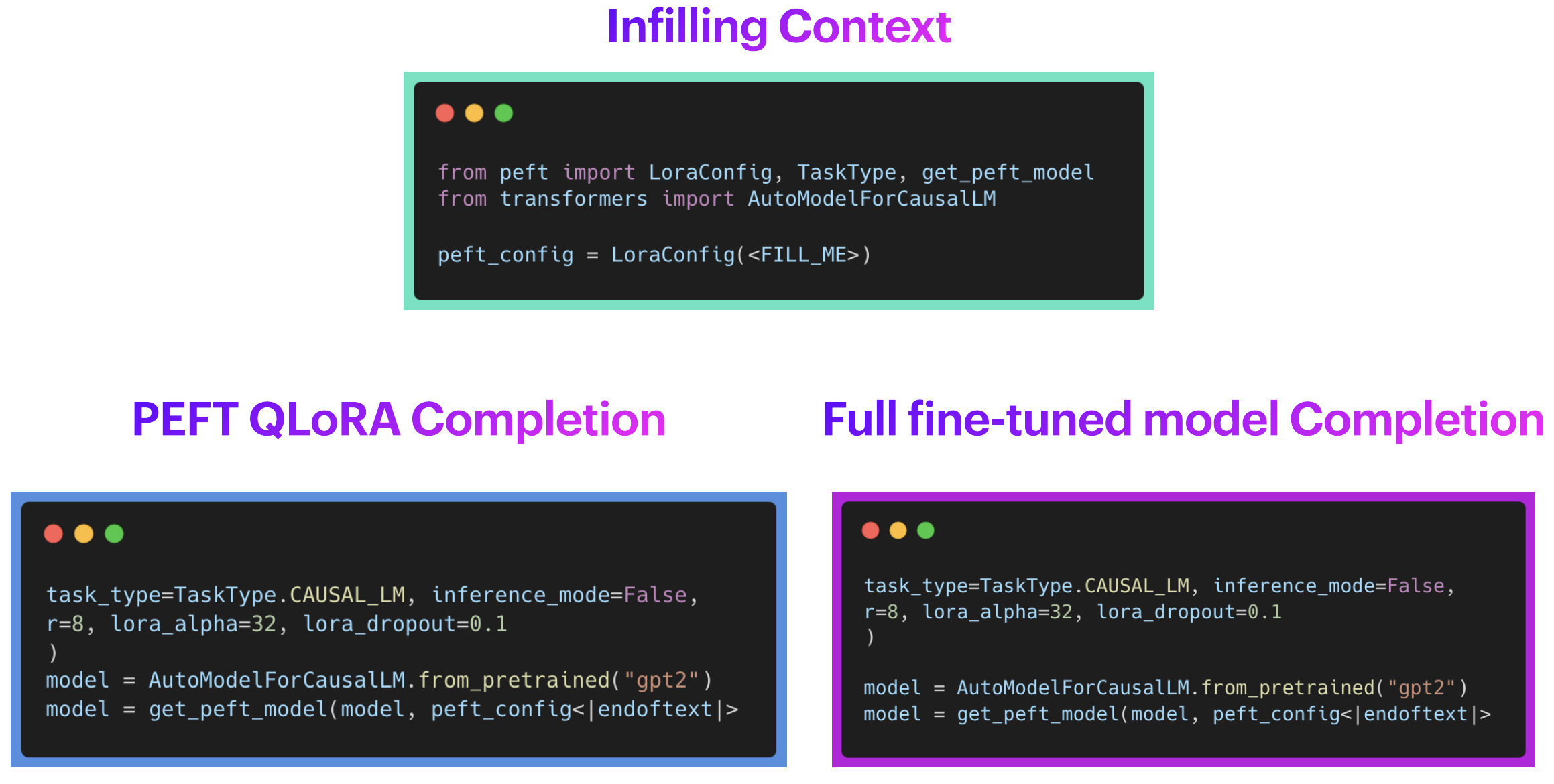 Qualitative Example 2 In the second example above, **GitHub Copilot didn't give any completion**. This can be due to the fact that 🤗 PEFT is a recent library and not yet part of Copilot's training data, which **is exactly the type of problem we are trying to address**. On the other hand, completions from QLoRA and full fine-tuned models are correctly infilling the entire function call with the necessary parameters. Again, note that both the QLoRA and the full fine-tuned models are giving generations of similar quality. Inference Code with various examples for full fine-tuned model and peft model are available at [Full_Finetuned_StarCoder_Inference.ipynb](https://github.com/pacman100/DHS-LLM-Workshop/blob/main/personal_copilot/inference/Full_Finetuned_StarCoder_Inference.ipynb) and [PEFT_StarCoder_Inference.ipynb](https://github.com/pacman100/DHS-LLM-Workshop/blob/main/personal_copilot/inference/PEFT_StarCoder_Inference.ipynb), respectively. Therefore, we can observe that the generations from both the variants are as per expectations. Awesome! 🚀 ## How do I use it in VS Code? You can easily configure a custom code-completion LLM in VS Code using 🤗 [llm-vscode](https://marketplace.visualstudio.com/items?itemName=HuggingFace.huggingface-vscode) VS Code Extension, together with hosting the model via [🤗 Inference EndPoints](https://ui.endpoints.huggingface.co/). We'll go through the required steps below. You can learn more details about deploying an endpoint in the [inference endpoints documentation](https://huggingface.co/docs/inference-endpoints/index). ### Setting an Inference Endpoint Below are the screenshots with the steps we followed to create our custom Inference Endpoint. We used our QLoRA model, exported as a full-sized _merged_ model that can be easily loaded in `transformers`. 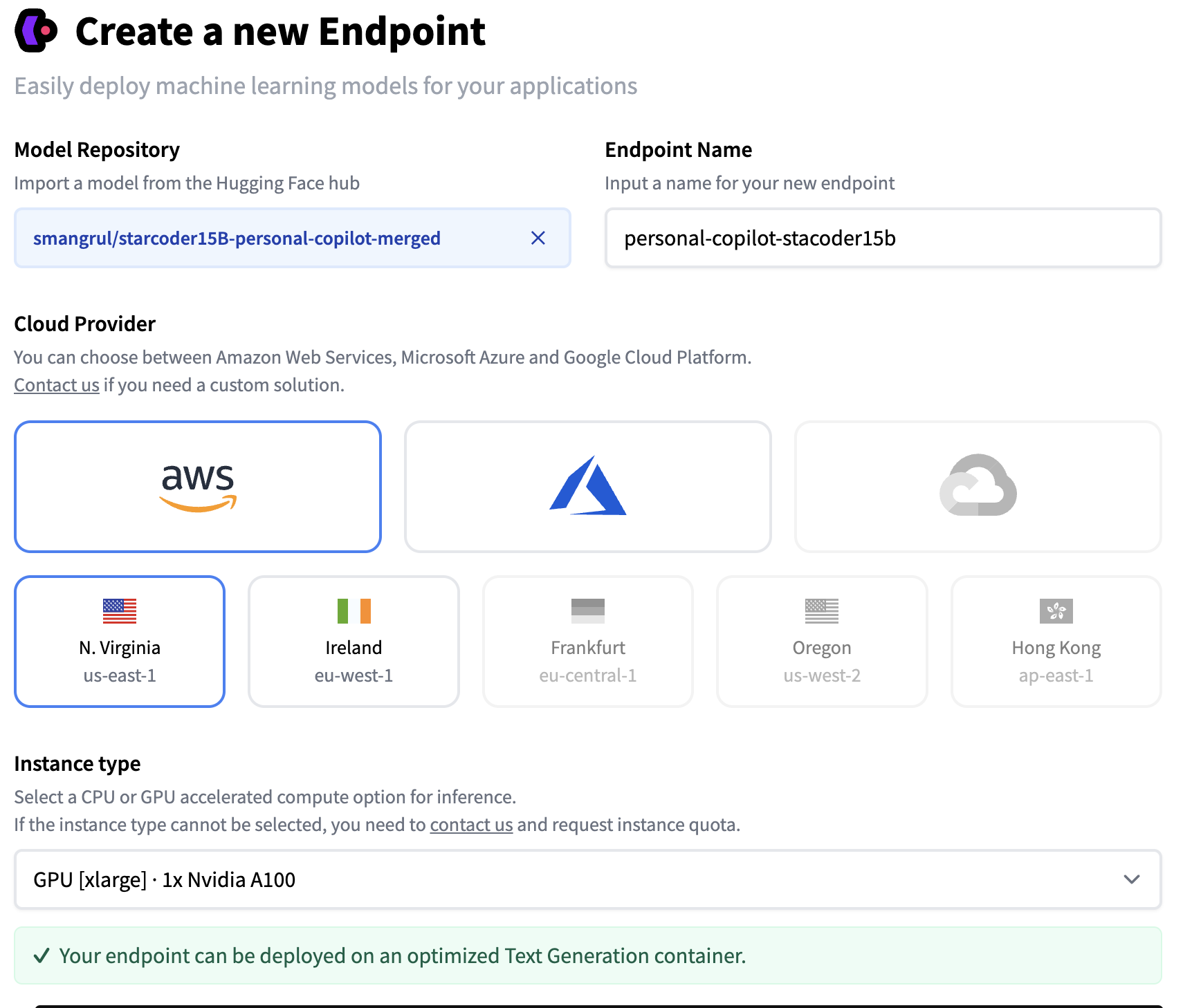 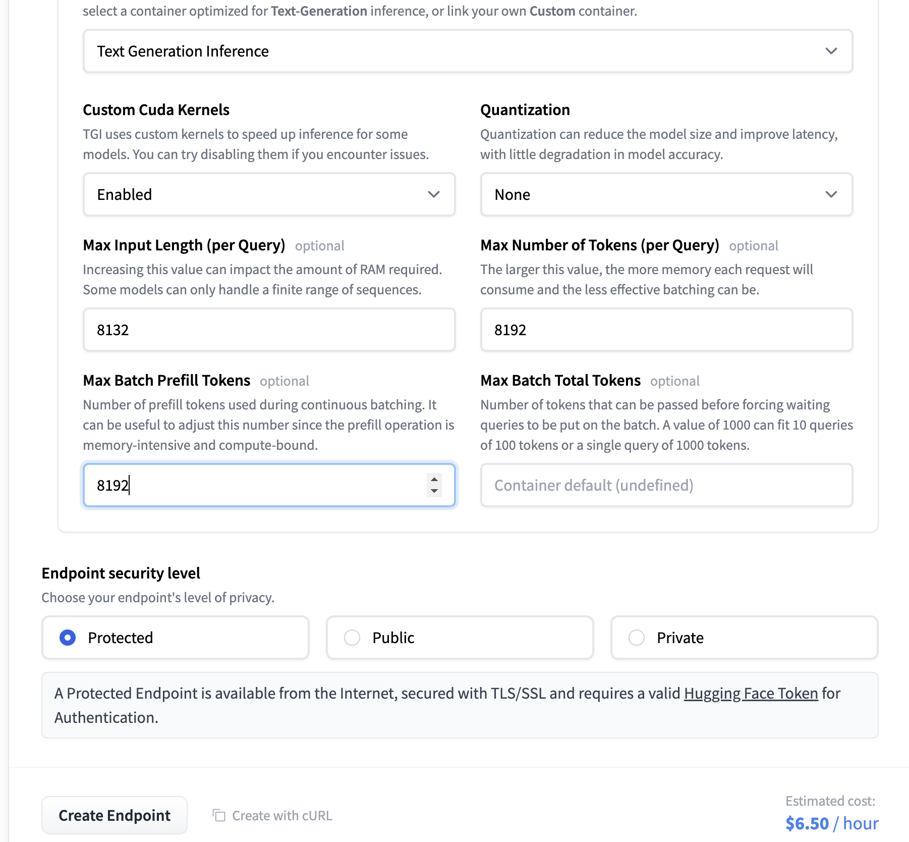 ### Setting up the VS Code Extension Just follow the [installation steps](https://github.com/huggingface/llm-vscode#installation). In the settings, replace the endpoint in the field below, so it points to the HF Inference Endpoint you deployed. 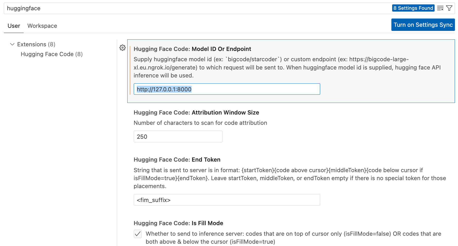 Usage will look like below: 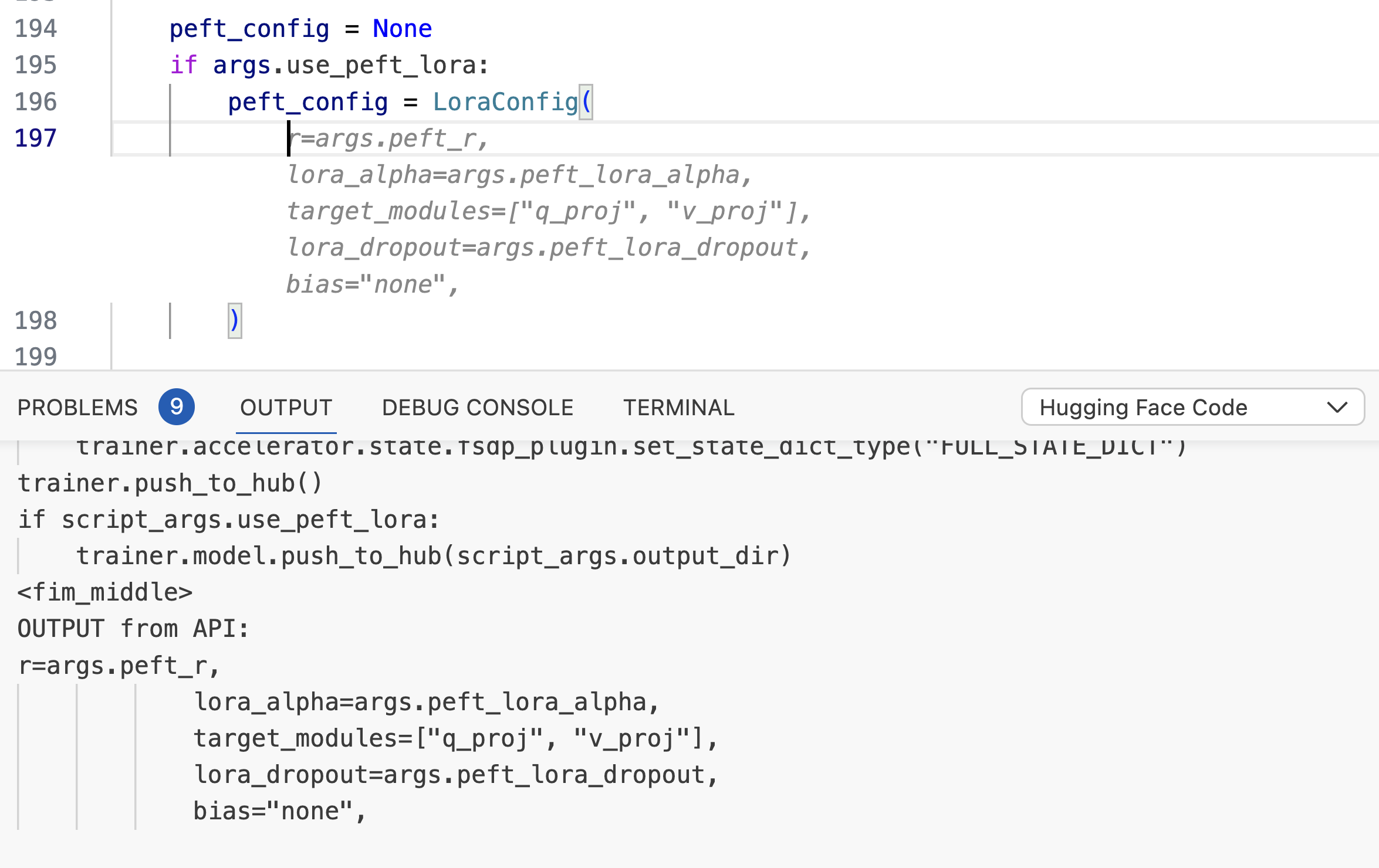 # Finetuning your own Code Chat Assistant So far, the models we trained were specifically trained as personal co-pilot for code completion tasks. They aren't trained to carry out conversations or for question answering. `Octocoder` and `StarChat` are great examples of such models. This section briefly describes how to achieve that. **Resources** 1. Codebase: [link](https://github.com/pacman100/DHS-LLM-Workshop/tree/main/code_assistant/training). It uses the recently added Flash Attention V2 support in Transformers. 2. Colab notebook: [link](https://colab.research.google.com/drive/1XFyePK-3IoyX81RM94JO73CcIZtAU4i4?usp=sharing). Make sure to choose A100 GPU with High RAM setting. 3. Model: [bigcode/stacoderplus](https://huggingface.co/bigcode/starcoderplus) 4. Dataset: [smangrul/code-chat-assistant-v1](https://huggingface.co/datasets/smangrul/code-chat-assistant-v1). Mix of `LIMA+GUANACO` with proper formatting in a ready-to-train format. 5. Trained Model: [smangrul/peft-lora-starcoderplus-chat-asst-A100-40GB-colab](https://huggingface.co/smangrul/peft-lora-starcoderplus-chat-asst-A100-40GB-colab) # Dance of LoRAs If you have dabbled with Stable Diffusion models and LoRAs for making your own Dreambooth models, you might be familiar with the concepts of combining different LoRAs with different weights, using a LoRA model with a different base model than the one on which it was trained. In text/code domain, this remains unexplored territory. We carry out experiments in this regard and have observed very promising findings. Are you ready? Let's go! 🚀 ## Mix-and-Match LoRAs PEFT currently supports 3 ways of combining LoRA models, `linear`, `svd` and `cat`. For more details, refer to [tuners#peft.LoraModel.add_weighted_adapter](https://huggingface.co/docs/peft/main/en/package_reference/tuners#peft.LoraModel.add_weighted_adapter). Our notebook [Dance_of_LoRAs.ipynb](https://github.com/pacman100/DHS-LLM-Workshop/blob/main/personal_copilot/inference/Dance_of_LoRAs.ipynb) includes all the inference code and various LoRA loading combinations, like loading the chat assistant on top of `starcoder` instead of `starcodeplus`, which is the base model that we fine-tuned. Here, we will consider 2 abilities (`chatting/QA` and `code-completion`) on 2 data distributions (`top 10 public hf codebase` and `generic codebase`). That gives us 4 axes on which we'll carry out some qualitative evaluation analyses. #### First, let us consider the `chatting/QA` task. If we disable adapters, we observe that the task fails for both datasets, as the base model (`starcoder`) is only meant for code completion and not suitable for `chatting/question-answering`. Enabling `copilot` adapter performs similar to the disabled case because this LoRA was also specifically fine-tuned for code-completion. Now, let's enable the `assistant` adapter. 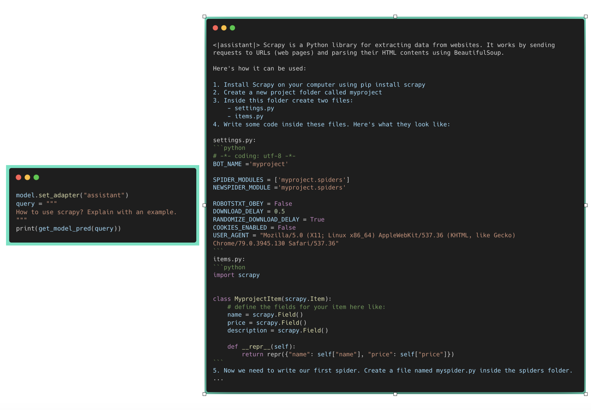 Question Answering based on generic code  Question Answering based on HF code We can observe that generic question regarding `scrapy` is being answered properly. However, it is failing for the HF code related question which wasn't part of its pretraining data. ##### Let us now consider the `code-completion` task. On disabling adapters, we observe that the code completion for the generic two-sum works as expected. However, the HF code completion fails with wrong params to `LoraConfig`, because the base model hasn't seen it in its pretraining data. Enabling `assistant` performs similar to the disabled case as it was trained on natural language conversations which didn't have any Hugging Face code repos. Now, let's enable the `copilot` adapter. 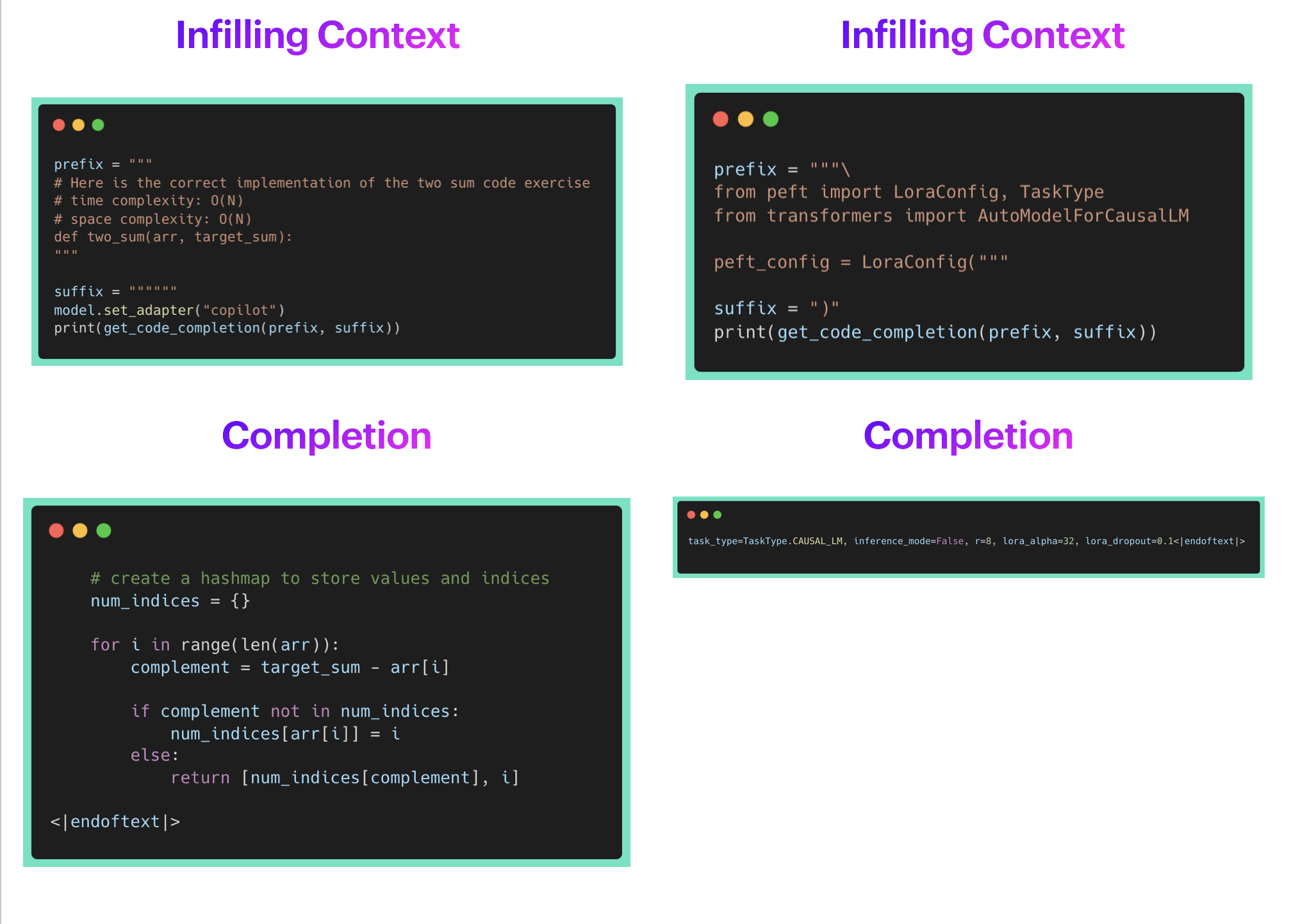 We can observe that the `copilot` adapter gets it right in both cases. Therefore, it performs as expected for code-completions when working with HF specific codebase as well as generic codebases. **Now, as a user, I want to combine the ability of `assistant` as well as `copilot`. This will enable me to use it for code completion while coding in an IDE, and also have it as a chatbot to answer my questions regarding APIs, classes, methods, documentation. It should be able to provide answers to questions like `How do I use x`, `Please write a code snippet for Y` on my codebase.** PEFT allows you to do it via `add_weighted_adapter`. Let's create a new adapter `code_buddy` with equal weights to `assistant` and `copilot` adapters. 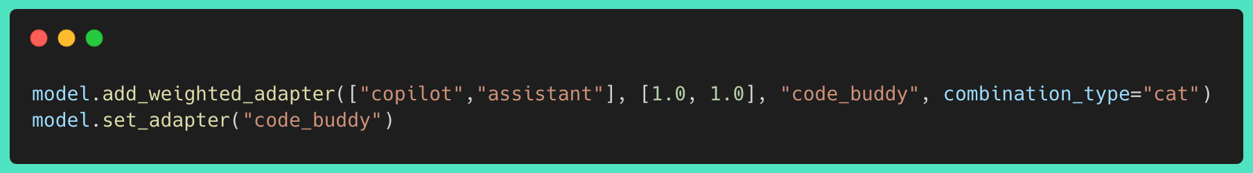 Combining Multiple Adapters Now, let's see how `code_buddy` performs on the `chatting/question_answering` tasks. 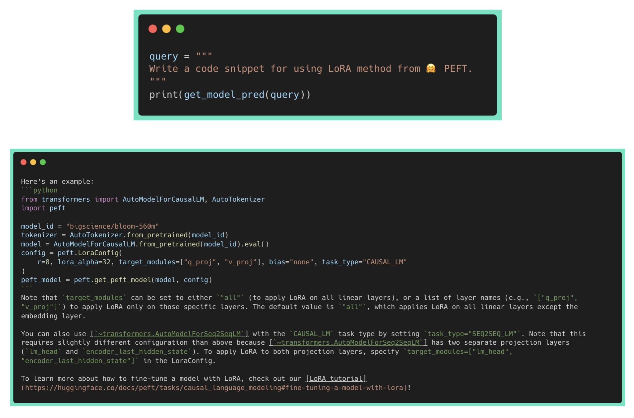 We can observe that `code_buddy` is performing much better than the `assistant` or `copilot` adapters alone! It is able to answer the _write a code snippet_ request to show how to use a specific HF repo API. However, it is also hallucinating the wrong links/explanations, which remains an open challenge for LLMs. Below is the performance of `code_buddy` on code completion tasks. 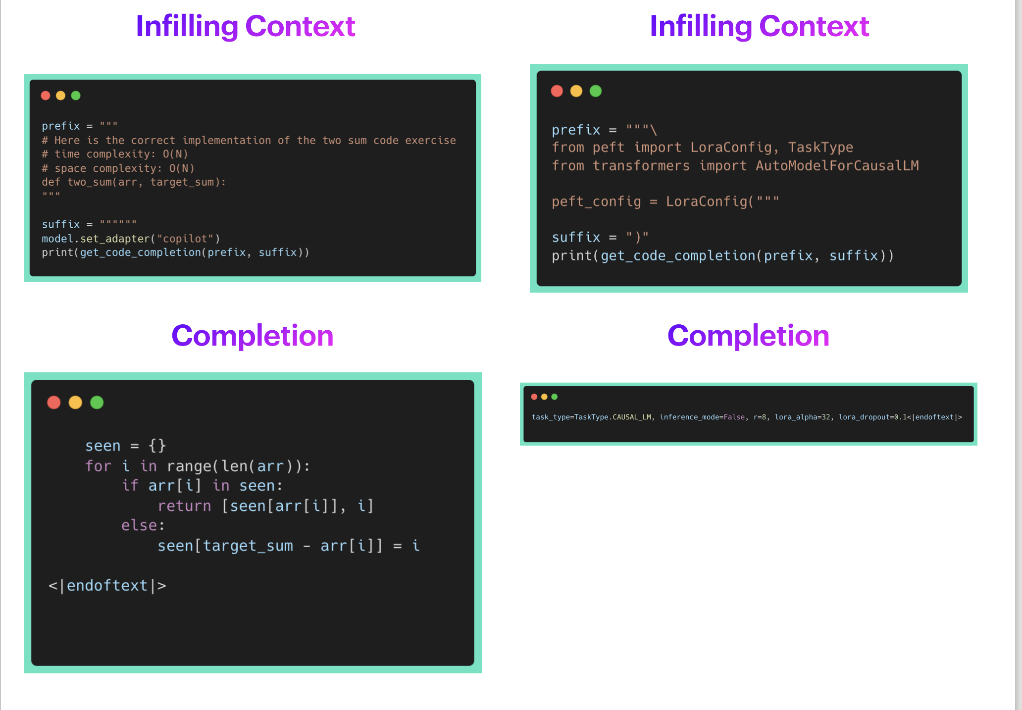 We can observe that `code_buddy` is performing on par with `copilot`, which was specifically finetuned for this task. ## Transfer LoRAs to different base models We can also transfer the LoRA models to different base models. We will take the hot-off-the-press `Octocoder` model and apply on it the LoRA we trained above with `starcoder` base model. Please go through the following notebook [PEFT_Personal_Code_CoPilot_Adapter_Transfer_Octocoder.ipynb](https://github.com/pacman100/DHS-LLM-Workshop/blob/main/personal_copilot/inference/PEFT_Personal_Code_CoPilot_Adapter_Transfer_Octocoder.ipynb) for the entire code. **Performance on the Code Completion task** 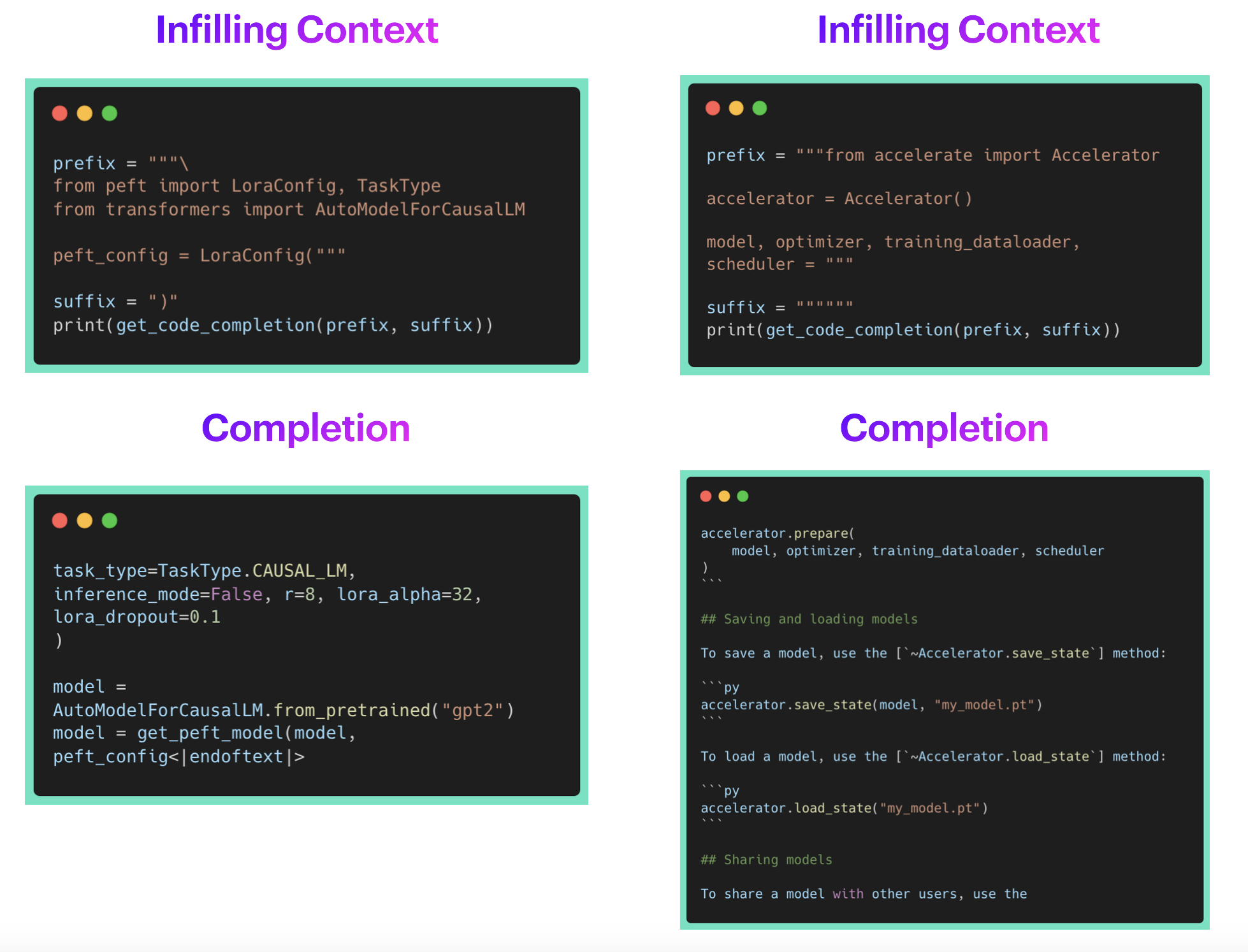 We can observe that `octocoder` is performing great. It is able to complete HF specific code snippets. It is also able to complete generic code snippets as seen in the notebook. **Performance on the Chatting/QA task** As Octocoder is trained to answer questions and carry out conversations about coding, let's see if it can use our LoRA adapter to answer HF specific questions. 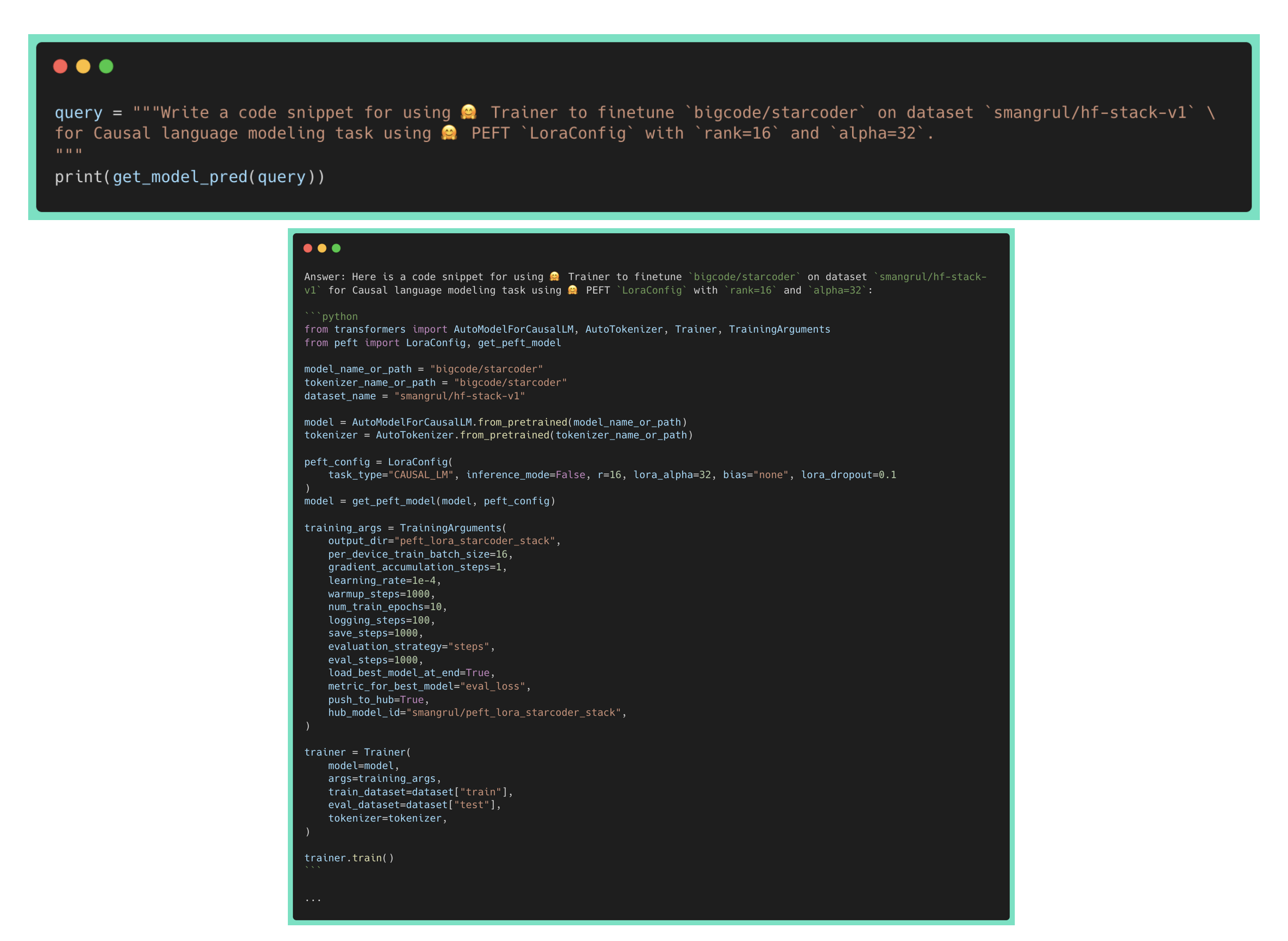 Yay! It correctly answers in detail how to create `LoraConfig` and related peft model along with correctly using the model name, dataset name as well as param values of LoraConfig. On disabling the adapter, it fails to correctly use the API of `LoraConfig` or to create a PEFT model, suggesting that it isn't part of the training data of Octocoder. # How do I run it locally? I know, after all this, you want to finetune starcoder on your codebase and use it locally on your consumer hardware such as Mac laptops with M1 GPUs, windows with RTX 4090/3090 GPUs ... Don't worry, we have got you covered. We will be using this super cool open source library [mlc-llm](https://github.com/mlc-ai/mlc-llm) 🔥. Specifically, we will be using this fork [pacman100/mlc-llm](https://github.com/pacman100/mlc-llm) which has changes to get it working with the Hugging Face Code Completion extension for VS Code. On my Mac latop with M1 Metal GPU, the 15B model was painfully slow. Hence, we will go small and train a PEFT LoRA version as well as a full finetuned version of `bigcode/starcoderbase-1b`. The training colab notebooks are linked below: 1. Colab notebook for Full fine-tuning and PEFT LoRA finetuning of `starcoderbase-1b`: [link](https://colab.research.google.com/drive/1tTdvc2buL3Iy1PKwrG_bBIDP06DC9r5m?usp=sharing) The training loss, evaluation loss as well as learning rate schedules are plotted below: 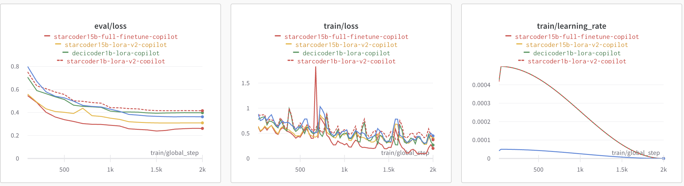 Now, we will look at detailed steps for locally hosting the merged model [smangrul/starcoder1B-v2-personal-copilot-merged](https://huggingface.co/smangrul/starcoder1B-v2-personal-copilot-merged) and using it with 🤗 [llm-vscode](https://marketplace.visualstudio.com/items?itemName=HuggingFace.huggingface-vscode) VS Code Extension. 1. Clone the repo ``` git clone --recursive https://github.com/pacman100/mlc-llm.git && cd mlc-llm/ ``` 2. Install the mlc-ai and mlc-chat (in editable mode) : ``` pip install --pre --force-reinstall mlc-ai-nightly mlc-chat-nightly -f https://mlc.ai/wheels cd python pip uninstall mlc-chat-nightly pip install -e ""."" ``` 3. Compile the model via: ``` time python3 -m mlc_llm.build --hf-path smangrul/starcoder1B-v2-personal-copilot-merged --target metal --use-cache=0 ``` 4. Update the config with the following values in `dist/starcoder1B-v2-personal-copilot-merged-q4f16_1/params/mlc-chat-config.json`: ```diff { ""model_lib"": ""starcoder7B-personal-copilot-merged-q4f16_1"", ""local_id"": ""starcoder7B-personal-copilot-merged-q4f16_1"", ""conv_template"": ""code_gpt"", - ""temperature"": 0.7, + ""temperature"": 0.2, - ""repetition_penalty"": 1.0, ""top_p"": 0.95, - ""mean_gen_len"": 128, + ""mean_gen_len"": 64, - ""max_gen_len"": 512, + ""max_gen_len"": 64, ""shift_fill_factor"": 0.3, ""tokenizer_files"": [ ""tokenizer.json"", ""merges.txt"", ""vocab.json"" ], ""model_category"": ""gpt_bigcode"", ""model_name"": ""starcoder1B-v2-personal-copilot-merged"" } ``` 5. Run the local server: ``` python -m mlc_chat.rest --model dist/starcoder1B-v2-personal-copilot-merged-q4f16_1/params --lib-path dist/starcoder1B-v2-personal-copilot-merged-q4f16_1/starcoder1B-v2-personal-copilot-merged-q4f16_1-metal.so ``` 6. Change the endpoint of HF Code Completion extension in VS Code to point to the local server: 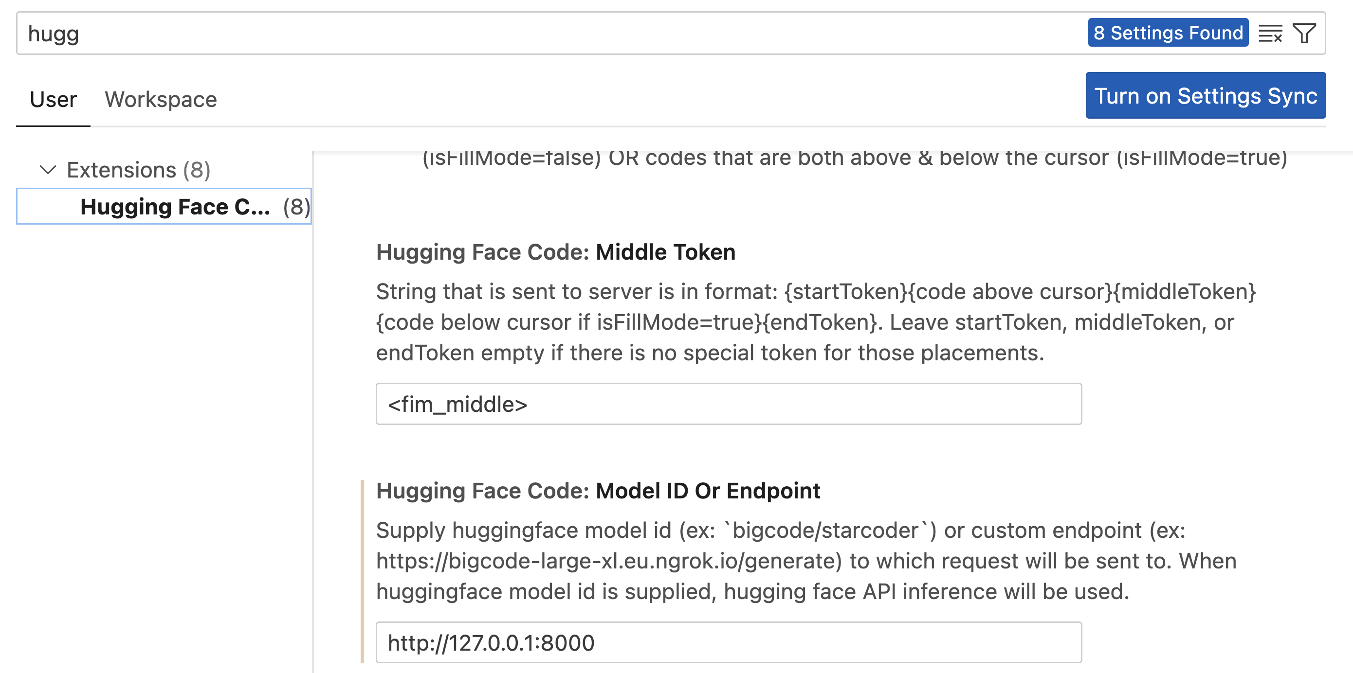 7. Open a new file in VS code, paste the code below and have the cursor in-between the doc quotes, so that the model tries to infill the doc string: 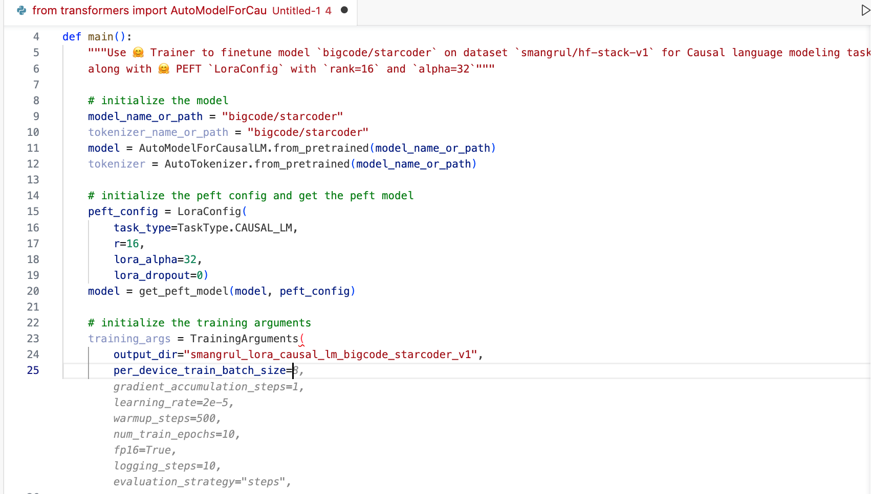 Voila! ⭐️ The demo at the start of this post is this 1B model running locally on my Mac laptop. ## Conclusion In this blog plost, we saw how to finetune `starcoder` to create a personal co-pilot that knows about our code. We called it 🤗 HugCoder, as we trained it on Hugging Face code :) After looking at the data collection workflow, we compared training using QLoRA vs full fine-tuning. We also experimented by combining different LoRAs, which is still an unexplored technique in the text/code domain. For deployment, we examined remote inference using 🤗 Inference Endpoints, and also showed on-device execution of a smaller model with VS Code and MLC. Please, let us know if you use these methods for your own codebase! ## Acknowledgements We would like to thank [Pedro Cuenca](https://github.com/pcuenca), [Leandro von Werra](https://github.com/lvwerra), [Benjamin Bossan](https://github.com/BenjaminBossan), [Sylvain Gugger](https://github.com/sgugger) and [Loubna Ben Allal](https://github.com/loubnabnl) for their help with the writing of this blogpost."
Creating open machine learning datasets? Share them on the Hugging Face Hub!,davanstrien,"October 30, 2023",researcher-dataset-sharing,"community, research, datasets, guide",https://huggingface.co/blog/researcher-dataset-sharing," # Creating open machine learning datasets? Share them on the Hugging Face Hub! ## Who is this blog post for? Are you a researcher doing data-intensive research or using machine learning as a research tool? As part of this research, you have likely created datasets for training and evaluating machine learning models, and like many researchers, you may be sharing these datasets via Google Drive, OneDrive, or your own personal server. In this post, we’ll outline why you might want to consider sharing these datasets on the Hugging Face Hub instead. This post outlines: - Why researchers should openly share their data (feel free to skip this section if you are already convinced about this!) - What the Hugging Face Hub offers for researchers who want to share their datasets. - Resources for getting started with sharing your datasets on the Hugging Face Hub. ## Why share your data? Machine learning is increasingly utilized across various disciplines, enhancing research efficiency in tackling diverse problems. Data remains crucial for training and evaluating models, especially when developing new machine-learning methods for specific tasks or domains. Large Language Models may not perform well on specialized tasks like bio-medical entity extraction, and computer vision models might struggle with classifying domain specific images. Domain-specific datasets are vital for evaluating and training machine learning models, helping to overcome the limitations of existing models. Creating these datasets, however, is challenging, requiring significant time, resources, and domain expertise, particularly for annotating data. Maximizing the impact of this data is crucial for the benefit of both the researchers involved and their respective fields. The Hugging Face Hub can help achieve this maximum impact. ## What is the Hugging Face Hub? The [Hugging Face Hub](https://huggingface.co/) has become the central hub for sharing open machine learning models, datasets and demos, hosting over 360,000 models and 70,000 datasets. The Hub enables people – including researchers – to access state-of-the-art machine learning models and datasets in a few lines of code.
## What’s next? With Spotlight you can create **interactive visualizations** and leverage data enrichments to **identify critical clusters** in your Hugging Face datasets. In this blog, we have seen both an audio ML and a computer vision example. You can use Spotlight directly to explore and curate your NLP, audio, CV or multimodal dataset: - Install Spotlight: *pip install renumics-spotlight* - Check out the [documentation](https://renumics.com/docs) or open an issue on [Github](https://github.com/Renumics/spotlight) - Join the [Spotlight community](https://discord.gg/VAQdFCU5YD) on Discord - Follow us on [Twitter](https://twitter.com/renumics) and [LinkedIn](https://www.linkedin.com/company/renumics)"
Personal Copilot: Train Your Own Coding Assistant,smangrul,"October 27, 2023",personal-copilot,"bigcode, llm, nlp, inference, guide",https://huggingface.co/blog/personal-copilot," # Personal Copilot: Train Your Own Coding Assistant In the ever-evolving landscape of programming and software development, the quest for efficiency and productivity has led to remarkable innovations. One such innovation is the emergence of code generation models such as [Codex](https://openai.com/blog/openai-codex), [StarCoder](https://arxiv.org/abs/2305.06161) and [Code Llama](https://arxiv.org/abs/2308.12950). These models have demonstrated remarkable capabilities in generating human-like code snippets, thereby showing immense potential as coding assistants. However, while these pre-trained models can perform impressively across a range of tasks, there's an exciting possibility lying just beyond the horizon: the ability to tailor a code generation model to your specific needs. Think of personalized coding assistants which could be leveraged at an enterprise scale. In this blog post we show how we created HugCoder 🤗, a code LLM fine-tuned on the code contents from the public repositories of the [`huggingface` GitHub organization](https://github.com/huggingface). We will discuss our data collection workflow, our training experiments, and some interesting results. This will enable you to create your own personal copilot based on your proprietary codebase. We will leave you with a couple of further extensions of this project for experimentation. Let’s begin 🚀  ## Data Collection Workflow Our desired dataset is conceptually simple, we structured it like so: | | | | |---|---|---| | Repository Name | Filepath in the Repository | File Contents | |---|---|---| |---|---|---| Scraping code contents from GitHub is straightforward with the [Python GitHub API](https://github.com/PyGithub/PyGithub). However, depending on the number of repositories and the number of code files within a repository, one might easily run into API rate-limiting issues. To prevent such problems, we decided to clone all the public repositories locally and extract the contents from them instead of through the API. We used the `multiprocessing` module from Python to download all repos in parallel, as shown in [this download script](https://github.com/sayakpaul/hf-codegen/blob/main/data/parallel_clone_repos.py). A repository can often contain non-code files such as images, presentations and other assets. We’re not interested in scraping them. We created a [list of extensions](https://github.com/sayakpaul/hf-codegen/blob/f659eba76f07e622873211e5b975168b634e6c22/data/prepare_dataset.py#L17C1-L49C68) to filter them out. To parse code files other than Jupyter Notebooks, we simply used the ""utf-8"" encoding. For notebooks, we only considered the code cells. We also excluded all file paths that were not directly related to code. These include: `.git`, `__pycache__`, and `xcodeproj`. To keep the serialization of this content relatively memory-friendly, we used chunking and the [feather format](https://arrow.apache.org/docs/python/feather.html#:~:text=Feather%20is%20a%20portable%20file,Python%20(pandas)%20and%20R.). Refer to [this script](https://github.com/sayakpaul/hf-codegen/blob/main/data/prepare_dataset.py) for the full implementation. The final dataset is [available on the Hub](https://huggingface.co/datasets/sayakpaul/hf-codegen-v2), and it looks like this:  For this blog, we considered the top 10 Hugging Face public repositories, based on stargazers. They are the following: > ['transformers', 'pytorch-image-models', 'datasets', 'diffusers', 'peft', 'tokenizers', 'accelerate', 'text-generation-inference', 'chat-ui', 'deep-rl-class'] [This is the code we used to generate this dataset](https://github.com/pacman100/DHS-LLM-Workshop/tree/main/personal_copilot/dataset_generation), and [this is the dataset in the Hub](https://huggingface.co/datasets/smangrul/hf-stack-v1). Here is a snapshot of what it looks like:  To reduce the project complexity, we didn’t consider deduplication of the dataset. If you are interested in applying deduplication techniques for a production application, [this blog post](https://huggingface.co/blog/dedup) is an excellent resource about the topic in the context of code LLMs. ## Finetuning your own Personal Co-Pilot In this section, we show how to fine-tune the following models: [`bigcode/starcoder`](https://hf.co/bigcode/starcoder) (15.5B params), [`bigcode/starcoderbase-1b`](https://hf.co/bigcode/starcoderbase-1b) (1B params), [`Deci/DeciCoder-1b`](https://hf.co/Deci/DeciCoder-1b) (1B params). We'll use a single A100 40GB Colab Notebook using 🤗 PEFT (Parameter-Efficient Fine-Tuning) for all the experiments. Additionally, we'll show how to fully finetune the `bigcode/starcoder` (15.5B params) on a machine with 8 A100 80GB GPUs using 🤗 Accelerate's FSDP integration. The training objective is [fill in the middle (FIM)](https://arxiv.org/abs/2207.14255), wherein parts of a training sequence are moved to the end, and the reordered sequence is predicted auto-regressively. Why PEFT? Full fine-tuning is expensive. Let’s have some numbers to put things in perspective: Minimum GPU memory required for full fine-tuning: 1. Weight: 2 bytes (Mixed-Precision training) 2. Weight gradient: 2 bytes 3. Optimizer state when using Adam: 4 bytes for original FP32 weight + 8 bytes for first and second moment estimates 4. Cost per parameter adding all of the above: 16 bytes per parameter 5. **15.5B model -> 248GB of GPU memory without even considering huge memory requirements for storing intermediate activations -> minimum 4X A100 80GB GPUs required** Since the hardware requirements are huge, we'll be using parameter-efficient fine-tuning using [QLoRA](https://arxiv.org/abs/2305.14314). Here are the minimal GPU memory requirements for fine-tuning StarCoder using QLoRA: > trainable params: 110,428,160 || all params: 15,627,884,544 || trainable%: 0.7066097761926236 1. Base model Weight: 0.5 bytes * 15.51B frozen params = 7.755 GB 2. Adapter weight: 2 bytes * 0.11B trainable params = 0.22GB 3. Weight gradient: 2 bytes * 0.11B trainable params = 0.12GB 4. Optimizer state when using Adam: 4 bytes * 0.11B trainable params * 3 = 1.32GB 5. **Adding all of the above -> 9.51 GB ~10GB -> 1 A100 40GB GPU required** 🤯. The reason for A100 40GB GPU is that the intermediate activations for long sequence lengths of 2048 and batch size of 4 for training lead to higher memory requirements. As we will see below, GPU memory required is 26GB which can be accommodated on A100 40GB GPU. Also, A100 GPUs have better compatibilty with Flash Attention 2. In the above calculations, we didn't consider memory required for intermediate activation checkpointing which is considerably huge. We leverage Flash Attention V2 and Gradient Checkpointing to overcome this issue. 1. For QLoRA along with flash attention V2 and gradient checkpointing, the total memory occupied by the model on a single A100 40GB GPU is **26 GB** with a **batch size of 4**. 2. For full fine-tuning using FSDP along with Flash Attention V2 and Gradient Checkpointing, the memory occupied per GPU ranges between **70 GB to 77.6 GB** with a **per_gpu_batch_size of 1**. Please refer to the [model-memory-usage](https://huggingface.co/spaces/hf-accelerate/model-memory-usage) to easily calculate how much vRAM is needed to train and perform big model inference on a model hosted on the 🤗 Hugging Face Hub. ## Full Finetuning We will look at how to do full fine-tuning of `bigcode/starcoder` (15B params) on 8 A100 80GB GPUs using PyTorch Fully Sharded Data Parallel (FSDP) technique. For more information on FSDP, please refer to [Fine-tuning Llama 2 70B using PyTorch FSDP](https://huggingface.co/blog/ram-efficient-pytorch-fsdp) and [Accelerate Large Model Training using PyTorch Fully Sharded Data Parallel](https://huggingface.co/blog/pytorch-fsdp). **Resources** 1. Codebase: [link](https://github.com/pacman100/DHS-LLM-Workshop/tree/main/personal_copilot/training). It uses the recently added Flash Attention V2 support in Transformers. 2. FSDP Config: [fsdp_config.yaml](https://github.com/pacman100/DHS-LLM-Workshop/blob/main/personal_copilot/training/configs/fsdp_config.yaml) 3. Model: [bigcode/stacoder](https://huggingface.co/bigcode/starcoder) 4. Dataset: [smangrul/hf-stack-v1](https://huggingface.co/datasets/smangrul/hf-stack-v1) 5. Fine-tuned Model: [smangrul/peft-lora-starcoder15B-v2-personal-copilot-A100-40GB-colab](https://huggingface.co/smangrul/peft-lora-starcoder15B-v2-personal-copilot-A100-40GB-colab) The command to launch training is given at [run_fsdp.sh](https://github.com/pacman100/DHS-LLM-Workshop/blob/main/personal_copilot/training/run_fsdp.sh). ``` accelerate launch --config_file ""configs/fsdp_config.yaml"" train.py \ --model_path ""bigcode/starcoder"" \ --dataset_name ""smangrul/hf-stack-v1"" \ --subset ""data"" \ --data_column ""content"" \ --split ""train"" \ --seq_length 2048 \ --max_steps 2000 \ --batch_size 1 \ --gradient_accumulation_steps 2 \ --learning_rate 5e-5 \ --lr_scheduler_type ""cosine"" \ --weight_decay 0.01 \ --num_warmup_steps 30 \ --eval_freq 100 \ --save_freq 500 \ --log_freq 25 \ --num_workers 4 \ --bf16 \ --no_fp16 \ --output_dir ""starcoder-personal-copilot-A100-40GB-colab"" \ --fim_rate 0.5 \ --fim_spm_rate 0.5 \ --use_flash_attn ``` The total training time was **9 Hours**. Taking the cost of $12.00 / hr based on [lambdalabs](https://lambdalabs.com/service/gpu-cloud/pricing) for 8x A100 80GB GPUs, the total cost would be **$108**. ## PEFT We will look at how to use QLoRA for fine-tuning `bigcode/starcoder` (15B params) on a single A100 40GB GPU using 🤗 PEFT. For more information on QLoRA and PEFT methods, please refer to [Making LLMs even more accessible with bitsandbytes, 4-bit quantization and QLoRA](https://huggingface.co/blog/4bit-transformers-bitsandbytes) and [🤗 PEFT: Parameter-Efficient Fine-Tuning of Billion-Scale Models on Low-Resource Hardware](https://huggingface.co/blog/peft). **Resources** 1. Codebase: [link](https://github.com/pacman100/DHS-LLM-Workshop/tree/main/personal_copilot/training). It uses the recently added Flash Attention V2 support in Transformers. 2. Colab notebook: [link](https://colab.research.google.com/drive/1Tz9KKgacppA4S6H4eo_sw43qEaC9lFLs?usp=sharing). Make sure to choose A100 GPU with High RAM setting. 3. Model: [bigcode/stacoder](https://huggingface.co/bigcode/starcoder) 4. Dataset: [smangrul/hf-stack-v1](https://huggingface.co/datasets/smangrul/hf-stack-v1) 5. QLoRA Fine-tuned Model: [smangrul/peft-lora-starcoder15B-v2-personal-copilot-A100-40GB-colab](https://huggingface.co/smangrul/peft-lora-starcoder15B-v2-personal-copilot-A100-40GB-colab) The command to launch training is given at [run_peft.sh](https://github.com/pacman100/DHS-LLM-Workshop/blob/main/personal_copilot/training/run_peft.sh). The total training time was **12.5 Hours**. Taking the cost of **$1.10 / hr** based on [lambdalabs](https://lambdalabs.com/service/gpu-cloud/pricing), the total cost would be **$13.75**. That's pretty good 🚀! In terms of cost, it's **7.8X** lower than the cost for full fine-tuning. ## Comparison The plot below shows the eval loss, train loss and learning rate scheduler for QLoRA vs full fine-tuning. We observe that full fine-tuning leads to slightly lower loss and converges a bit faster compared to QLoRA. The learning rate for peft fine-tuning is 10X more than that of full fine-tuning.  To make sure that our QLoRA model doesn't lead to catastrophic forgetting, we run the Python Human Eval on it. Below are the results we got. `Pass@1` measures the pass rate of completions considering just a single generated code candidate per problem. We can observe that the performance on `humaneval-python` is comparable between the base `bigcode/starcoder` (15B params) and the fine-tuned PEFT model `smangrul/peft-lora-starcoder15B-v2-personal-copilot-A100-40GB-colab`. | | | |---|---| | Model | Pass@1 | |bigcode/starcoder | 33.57| |smangrul/peft-lora-starcoder15B-v2-personal-copilot-A100-40GB-colab| 33.37 | Let's now look at some qualitative samples. In our manual analysis, we noticed that the QLoRA led to slight overfitting and as such we down weigh it by creating new weighted adapter with weight 0.8 via `add_weighted_adapter` utility of PEFT. We will look at 2 code infilling examples wherein the task of the model is to fill the part denoted by the `` placeholder. We will consider infilling completions from GitHub Copilot, the QLoRA fine-tuned model and the full fine-tuned model.  *Qualitative Example 1* In the example above, the completion from GitHub Copilot is along the correct lines but doesn't help much. On the other hand, completions from QLoRA and full fine-tuned models are correctly infilling the entire function call with the necessary parameters. However, they are also adding a lot more noise afterwards. This could be controlled with a post-processing step to limit completions to closing brackets or new lines. Note that both QLoRA and full fine-tuned models produce results with similar quality.  Qualitative Example 2 In the second example above, **GitHub Copilot didn't give any completion**. This can be due to the fact that 🤗 PEFT is a recent library and not yet part of Copilot's training data, which **is exactly the type of problem we are trying to address**. On the other hand, completions from QLoRA and full fine-tuned models are correctly infilling the entire function call with the necessary parameters. Again, note that both the QLoRA and the full fine-tuned models are giving generations of similar quality. Inference Code with various examples for full fine-tuned model and peft model are available at [Full_Finetuned_StarCoder_Inference.ipynb](https://github.com/pacman100/DHS-LLM-Workshop/blob/main/personal_copilot/inference/Full_Finetuned_StarCoder_Inference.ipynb) and [PEFT_StarCoder_Inference.ipynb](https://github.com/pacman100/DHS-LLM-Workshop/blob/main/personal_copilot/inference/PEFT_StarCoder_Inference.ipynb), respectively. Therefore, we can observe that the generations from both the variants are as per expectations. Awesome! 🚀 ## How do I use it in VS Code? You can easily configure a custom code-completion LLM in VS Code using 🤗 [llm-vscode](https://marketplace.visualstudio.com/items?itemName=HuggingFace.huggingface-vscode) VS Code Extension, together with hosting the model via [🤗 Inference EndPoints](https://ui.endpoints.huggingface.co/). We'll go through the required steps below. You can learn more details about deploying an endpoint in the [inference endpoints documentation](https://huggingface.co/docs/inference-endpoints/index). ### Setting an Inference Endpoint Below are the screenshots with the steps we followed to create our custom Inference Endpoint. We used our QLoRA model, exported as a full-sized _merged_ model that can be easily loaded in `transformers`.   ### Setting up the VS Code Extension Just follow the [installation steps](https://github.com/huggingface/llm-vscode#installation). In the settings, replace the endpoint in the field below, so it points to the HF Inference Endpoint you deployed.  Usage will look like below:  # Finetuning your own Code Chat Assistant So far, the models we trained were specifically trained as personal co-pilot for code completion tasks. They aren't trained to carry out conversations or for question answering. `Octocoder` and `StarChat` are great examples of such models. This section briefly describes how to achieve that. **Resources** 1. Codebase: [link](https://github.com/pacman100/DHS-LLM-Workshop/tree/main/code_assistant/training). It uses the recently added Flash Attention V2 support in Transformers. 2. Colab notebook: [link](https://colab.research.google.com/drive/1XFyePK-3IoyX81RM94JO73CcIZtAU4i4?usp=sharing). Make sure to choose A100 GPU with High RAM setting. 3. Model: [bigcode/stacoderplus](https://huggingface.co/bigcode/starcoderplus) 4. Dataset: [smangrul/code-chat-assistant-v1](https://huggingface.co/datasets/smangrul/code-chat-assistant-v1). Mix of `LIMA+GUANACO` with proper formatting in a ready-to-train format. 5. Trained Model: [smangrul/peft-lora-starcoderplus-chat-asst-A100-40GB-colab](https://huggingface.co/smangrul/peft-lora-starcoderplus-chat-asst-A100-40GB-colab) # Dance of LoRAs If you have dabbled with Stable Diffusion models and LoRAs for making your own Dreambooth models, you might be familiar with the concepts of combining different LoRAs with different weights, using a LoRA model with a different base model than the one on which it was trained. In text/code domain, this remains unexplored territory. We carry out experiments in this regard and have observed very promising findings. Are you ready? Let's go! 🚀 ## Mix-and-Match LoRAs PEFT currently supports 3 ways of combining LoRA models, `linear`, `svd` and `cat`. For more details, refer to [tuners#peft.LoraModel.add_weighted_adapter](https://huggingface.co/docs/peft/main/en/package_reference/tuners#peft.LoraModel.add_weighted_adapter). Our notebook [Dance_of_LoRAs.ipynb](https://github.com/pacman100/DHS-LLM-Workshop/blob/main/personal_copilot/inference/Dance_of_LoRAs.ipynb) includes all the inference code and various LoRA loading combinations, like loading the chat assistant on top of `starcoder` instead of `starcodeplus`, which is the base model that we fine-tuned. Here, we will consider 2 abilities (`chatting/QA` and `code-completion`) on 2 data distributions (`top 10 public hf codebase` and `generic codebase`). That gives us 4 axes on which we'll carry out some qualitative evaluation analyses. #### First, let us consider the `chatting/QA` task. If we disable adapters, we observe that the task fails for both datasets, as the base model (`starcoder`) is only meant for code completion and not suitable for `chatting/question-answering`. Enabling `copilot` adapter performs similar to the disabled case because this LoRA was also specifically fine-tuned for code-completion. Now, let's enable the `assistant` adapter.  Question Answering based on generic code  Question Answering based on HF code We can observe that generic question regarding `scrapy` is being answered properly. However, it is failing for the HF code related question which wasn't part of its pretraining data. ##### Let us now consider the `code-completion` task. On disabling adapters, we observe that the code completion for the generic two-sum works as expected. However, the HF code completion fails with wrong params to `LoraConfig`, because the base model hasn't seen it in its pretraining data. Enabling `assistant` performs similar to the disabled case as it was trained on natural language conversations which didn't have any Hugging Face code repos. Now, let's enable the `copilot` adapter.  We can observe that the `copilot` adapter gets it right in both cases. Therefore, it performs as expected for code-completions when working with HF specific codebase as well as generic codebases. **Now, as a user, I want to combine the ability of `assistant` as well as `copilot`. This will enable me to use it for code completion while coding in an IDE, and also have it as a chatbot to answer my questions regarding APIs, classes, methods, documentation. It should be able to provide answers to questions like `How do I use x`, `Please write a code snippet for Y` on my codebase.** PEFT allows you to do it via `add_weighted_adapter`. Let's create a new adapter `code_buddy` with equal weights to `assistant` and `copilot` adapters.  Combining Multiple Adapters Now, let's see how `code_buddy` performs on the `chatting/question_answering` tasks.  We can observe that `code_buddy` is performing much better than the `assistant` or `copilot` adapters alone! It is able to answer the _write a code snippet_ request to show how to use a specific HF repo API. However, it is also hallucinating the wrong links/explanations, which remains an open challenge for LLMs. Below is the performance of `code_buddy` on code completion tasks.  We can observe that `code_buddy` is performing on par with `copilot`, which was specifically finetuned for this task. ## Transfer LoRAs to different base models We can also transfer the LoRA models to different base models. We will take the hot-off-the-press `Octocoder` model and apply on it the LoRA we trained above with `starcoder` base model. Please go through the following notebook [PEFT_Personal_Code_CoPilot_Adapter_Transfer_Octocoder.ipynb](https://github.com/pacman100/DHS-LLM-Workshop/blob/main/personal_copilot/inference/PEFT_Personal_Code_CoPilot_Adapter_Transfer_Octocoder.ipynb) for the entire code. **Performance on the Code Completion task**  We can observe that `octocoder` is performing great. It is able to complete HF specific code snippets. It is also able to complete generic code snippets as seen in the notebook. **Performance on the Chatting/QA task** As Octocoder is trained to answer questions and carry out conversations about coding, let's see if it can use our LoRA adapter to answer HF specific questions.  Yay! It correctly answers in detail how to create `LoraConfig` and related peft model along with correctly using the model name, dataset name as well as param values of LoraConfig. On disabling the adapter, it fails to correctly use the API of `LoraConfig` or to create a PEFT model, suggesting that it isn't part of the training data of Octocoder. # How do I run it locally? I know, after all this, you want to finetune starcoder on your codebase and use it locally on your consumer hardware such as Mac laptops with M1 GPUs, windows with RTX 4090/3090 GPUs ... Don't worry, we have got you covered. We will be using this super cool open source library [mlc-llm](https://github.com/mlc-ai/mlc-llm) 🔥. Specifically, we will be using this fork [pacman100/mlc-llm](https://github.com/pacman100/mlc-llm) which has changes to get it working with the Hugging Face Code Completion extension for VS Code. On my Mac latop with M1 Metal GPU, the 15B model was painfully slow. Hence, we will go small and train a PEFT LoRA version as well as a full finetuned version of `bigcode/starcoderbase-1b`. The training colab notebooks are linked below: 1. Colab notebook for Full fine-tuning and PEFT LoRA finetuning of `starcoderbase-1b`: [link](https://colab.research.google.com/drive/1tTdvc2buL3Iy1PKwrG_bBIDP06DC9r5m?usp=sharing) The training loss, evaluation loss as well as learning rate schedules are plotted below:  Now, we will look at detailed steps for locally hosting the merged model [smangrul/starcoder1B-v2-personal-copilot-merged](https://huggingface.co/smangrul/starcoder1B-v2-personal-copilot-merged) and using it with 🤗 [llm-vscode](https://marketplace.visualstudio.com/items?itemName=HuggingFace.huggingface-vscode) VS Code Extension. 1. Clone the repo ``` git clone --recursive https://github.com/pacman100/mlc-llm.git && cd mlc-llm/ ``` 2. Install the mlc-ai and mlc-chat (in editable mode) : ``` pip install --pre --force-reinstall mlc-ai-nightly mlc-chat-nightly -f https://mlc.ai/wheels cd python pip uninstall mlc-chat-nightly pip install -e ""."" ``` 3. Compile the model via: ``` time python3 -m mlc_llm.build --hf-path smangrul/starcoder1B-v2-personal-copilot-merged --target metal --use-cache=0 ``` 4. Update the config with the following values in `dist/starcoder1B-v2-personal-copilot-merged-q4f16_1/params/mlc-chat-config.json`: ```diff { ""model_lib"": ""starcoder7B-personal-copilot-merged-q4f16_1"", ""local_id"": ""starcoder7B-personal-copilot-merged-q4f16_1"", ""conv_template"": ""code_gpt"", - ""temperature"": 0.7, + ""temperature"": 0.2, - ""repetition_penalty"": 1.0, ""top_p"": 0.95, - ""mean_gen_len"": 128, + ""mean_gen_len"": 64, - ""max_gen_len"": 512, + ""max_gen_len"": 64, ""shift_fill_factor"": 0.3, ""tokenizer_files"": [ ""tokenizer.json"", ""merges.txt"", ""vocab.json"" ], ""model_category"": ""gpt_bigcode"", ""model_name"": ""starcoder1B-v2-personal-copilot-merged"" } ``` 5. Run the local server: ``` python -m mlc_chat.rest --model dist/starcoder1B-v2-personal-copilot-merged-q4f16_1/params --lib-path dist/starcoder1B-v2-personal-copilot-merged-q4f16_1/starcoder1B-v2-personal-copilot-merged-q4f16_1-metal.so ``` 6. Change the endpoint of HF Code Completion extension in VS Code to point to the local server:  7. Open a new file in VS code, paste the code below and have the cursor in-between the doc quotes, so that the model tries to infill the doc string:  Voila! ⭐️ The demo at the start of this post is this 1B model running locally on my Mac laptop. ## Conclusion In this blog plost, we saw how to finetune `starcoder` to create a personal co-pilot that knows about our code. We called it 🤗 HugCoder, as we trained it on Hugging Face code :) After looking at the data collection workflow, we compared training using QLoRA vs full fine-tuning. We also experimented by combining different LoRAs, which is still an unexplored technique in the text/code domain. For deployment, we examined remote inference using 🤗 Inference Endpoints, and also showed on-device execution of a smaller model with VS Code and MLC. Please, let us know if you use these methods for your own codebase! ## Acknowledgements We would like to thank [Pedro Cuenca](https://github.com/pcuenca), [Leandro von Werra](https://github.com/lvwerra), [Benjamin Bossan](https://github.com/BenjaminBossan), [Sylvain Gugger](https://github.com/sgugger) and [Loubna Ben Allal](https://github.com/loubnabnl) for their help with the writing of this blogpost."
Creating open machine learning datasets? Share them on the Hugging Face Hub!,davanstrien,"October 30, 2023",researcher-dataset-sharing,"community, research, datasets, guide",https://huggingface.co/blog/researcher-dataset-sharing," # Creating open machine learning datasets? Share them on the Hugging Face Hub! ## Who is this blog post for? Are you a researcher doing data-intensive research or using machine learning as a research tool? As part of this research, you have likely created datasets for training and evaluating machine learning models, and like many researchers, you may be sharing these datasets via Google Drive, OneDrive, or your own personal server. In this post, we’ll outline why you might want to consider sharing these datasets on the Hugging Face Hub instead. This post outlines: - Why researchers should openly share their data (feel free to skip this section if you are already convinced about this!) - What the Hugging Face Hub offers for researchers who want to share their datasets. - Resources for getting started with sharing your datasets on the Hugging Face Hub. ## Why share your data? Machine learning is increasingly utilized across various disciplines, enhancing research efficiency in tackling diverse problems. Data remains crucial for training and evaluating models, especially when developing new machine-learning methods for specific tasks or domains. Large Language Models may not perform well on specialized tasks like bio-medical entity extraction, and computer vision models might struggle with classifying domain specific images. Domain-specific datasets are vital for evaluating and training machine learning models, helping to overcome the limitations of existing models. Creating these datasets, however, is challenging, requiring significant time, resources, and domain expertise, particularly for annotating data. Maximizing the impact of this data is crucial for the benefit of both the researchers involved and their respective fields. The Hugging Face Hub can help achieve this maximum impact. ## What is the Hugging Face Hub? The [Hugging Face Hub](https://huggingface.co/) has become the central hub for sharing open machine learning models, datasets and demos, hosting over 360,000 models and 70,000 datasets. The Hub enables people – including researchers – to access state-of-the-art machine learning models and datasets in a few lines of code. ![]()
Datasets on the Hugging Face Hub.
## What does the Hugging Face Hub offer for data sharing? This blog post won’t cover all of the features and benefits of hosting datasets on the Hugging Face Hub but will instead highlight some that are particularly relevant for researchers. ### Visibility for your work The Hugging Face Hub has become the central Hub for people to collaborate on open machine learning. Making your datasets available via the Hugging Face Hub ensures it is visible to a wide audience of machine learning researchers. The Hub makes it possible to expose links between datasets, models and demos which makes it easier to see how people are using your datasets for training models and creating demos. ### Tools for exploring and working with datasets There are a growing number of tools being created which make it easier to understand datasets hosted on the Hugging Face Hub. ### Tools for loading datasets hosted on the Hugging Face Hub Datasets shared on the Hugging Face Hub can be loaded via a variety of tools. The [`datasets`](https://huggingface.co/docs/datasets/) library is a Python library which can directly load datasets from the huggingface hub via a `load_dataset` command. The `datasets` library is optimized for working with large datasets (including datasets which won't fit into memory) and supporting machine learning workflows. Alongside this many of the datasets on the Hub can also be loaded directly into [`Pandas`](https://pandas.pydata.org/), [`Polars`](https://www.pola.rs/), and [`DuckDB`](https://duckdb.org/). This [page](https://huggingface.co/docs/datasets-server/parquet_process) provides a more detailed overview of the different ways you can load datasets from the Hub. #### Datasets Viewer The datasets viewer allows people to explore and interact with datasets hosted on the Hub directly in the browser by visiting the dataset repository on the Hugging Face Hub. This makes it much easier for others to view and explore your data without first having to download it. The datasets viewer also allows you to search and filter datasets, which can be valuable to potential dataset users, understanding the nature of a dataset more quickly. ![]()
The dataset viewer for the multiconer_v2 Named Entity Recognition dataset.
### Community tools Alongside the datasets viewer there are a growing number of community created tools for exploring datasets on the Hub. #### Spotlight [`Spotlight`](https://github.com/Renumics/spotlight) is a tool that allows you to interactively explore datasets on the Hub with one line of code. ![]()
You can learn more about how you can use this tool in this [blog post](https://huggingface.co/blog/scalable-data-inspection). #### Lilac [`Lilac`](https://lilacml.com/) is a tool that aims to help you ""curate better data for LLMs"" and allows you to explore natural language datasets more easily. The tool allows you to semantically search your dataset (search by meaning), cluster data and gain high-level insights into your dataset. A Spaces demo of the lilac tool.
You can explore the `Lilac` tool further in a [demo](https://lilacai-lilac.hf.space/). This growing number of tools for exploring datasets on the Hub makes it easier for people to explore and understand your datasets and can help promote your datasets to a wider audience. ### Support for large datasets The Hub can host large datasets; it currently hosts datasets with multiple TBs of data.The datasets library, which users can use to download and process datasets from the Hub, supports streaming, making it possible to work with large datasets without downloading the entire dataset upfront. This can be invaluable for allowing researchers with less computational resources to work with your datasets, or to select small portions of a huge dataset for testing, development or prototyping. ![]()
The Hugging Face Hub can host the large datasets often created for machine learning research.
## API and client library interaction with the Hub Interacting with the Hugging Face Hub via an [API](https://huggingface.co/docs/hub/api) or the [`huggingface_hub`](https://huggingface.co/docs/huggingface_hub/index) Python library is possible. This includes creating new repositories, uploading data programmatically and creating and modifying metadata for datasets. This can be powerful for research workflows where new data or annotations continue to be created. The client library also makes uploading large datasets much more accessible. ## Community The Hugging Face Hub is already home to a large community of researchers, developers, artists, and others interested in using and contributing to an ecosystem of open-source machine learning. Making your datasets accessible to this community increases their visibility, opens them up to new types of users and places your datasets within the context of a larger ecosystem of models, datasets and libraries. The Hub also has features which allow communities to collaborate more easily. This includes a discussion page for each dataset, model and Space hosted on the Hub. This means users of your datasets can quickly ask questions and discuss ideas for working with a dataset. ![]()
The Hub makes it easy to ask questions and discuss datasets.
### Other important features for researchers Some other features of the Hub may be of particular interest to researchers wanting to share their machine learning datasets on the Hub: - [Organizations](https://huggingface.co/organizations) allow you to collaborate with other people and share models, datasets and demos under a single organization. This can be an excellent way of highlighting the work of a particular research project or institute. - [Gated repositories](https://huggingface.co/docs/hub/datasets-gated) allow you to add some access restrictions to accessing your dataset. - Download metrics are available for datasets on the Hub; this can be useful for communicating the impact of your researchers to funders and hiring committees. - [Digital Object Identifiers (DOI)](https://huggingface.co/docs/hub/doi): it’s possible to register a persistent identifier for your dataset. ### How can I share my dataset on the Hugging Face Hub? Here are some resources to help you get started with sharing your datasets on the Hugging Face Hub: - General guidance on [creating](https://huggingface.co/docs/datasets/create_dataset) and [sharing datasets on the Hub](https://huggingface.co/docs/datasets/upload_dataset) - Guides for particular modalities: - Creating an [audio dataset](https://huggingface.co/docs/datasets/audio_dataset) - Creating an [image dataset](https://huggingface.co/docs/datasets/image_dataset) - Guidance on [structuring your repository](https://huggingface.co/docs/datasets/repository_structure) so a dataset can be automatically loaded from the Hub. The following pages will be useful if you want to share large datasets: - [Repository limitations and recommendations](https://huggingface.co/docs/hub/repositories-recommendations) provides general guidance on some of the considerations you'll want to make when sharing large datasets. - The [Tips and tricks for large uploads](https://huggingface.co/docs/huggingface_hub/guides/upload#tips-and-tricks-for-large-uploads) page provides some guidance on how to upload large datasets to the Hub. If you want any further help uploading a dataset to the Hub or want to upload a particularly large dataset, please contact datasets@huggingface.co. "
Introducing Storage Regions on the HF Hub,julien-c,"November 3, 2023",regions,"announcement, enterprise, hub",https://huggingface.co/blog/regions," # Introducing Storage Regions on the Hub As part of our [Enterprise Hub](https://huggingface.co/enterprise) plan, we recently released support for **Storage Regions**. Regions let you decide where your org's models and datasets will be stored. This has two main benefits, which we'll briefly go over in this blog post: - **Regulatory and legal compliance**, and more generally, better digital sovereignty - **Performance** (improved download and upload speeds and latency) Currently we support the following regions: - US 🇺🇸 - EU 🇪🇺 - coming soon: Asia-Pacific 🌏 But first, let's see how to setup this feature in your organization's settings 🔥 ## Org settings If your organization is not an Enterprise Hub org yet, you will see the following screen:  As soon as you subscribe, you will be able to see the Regions settings page: 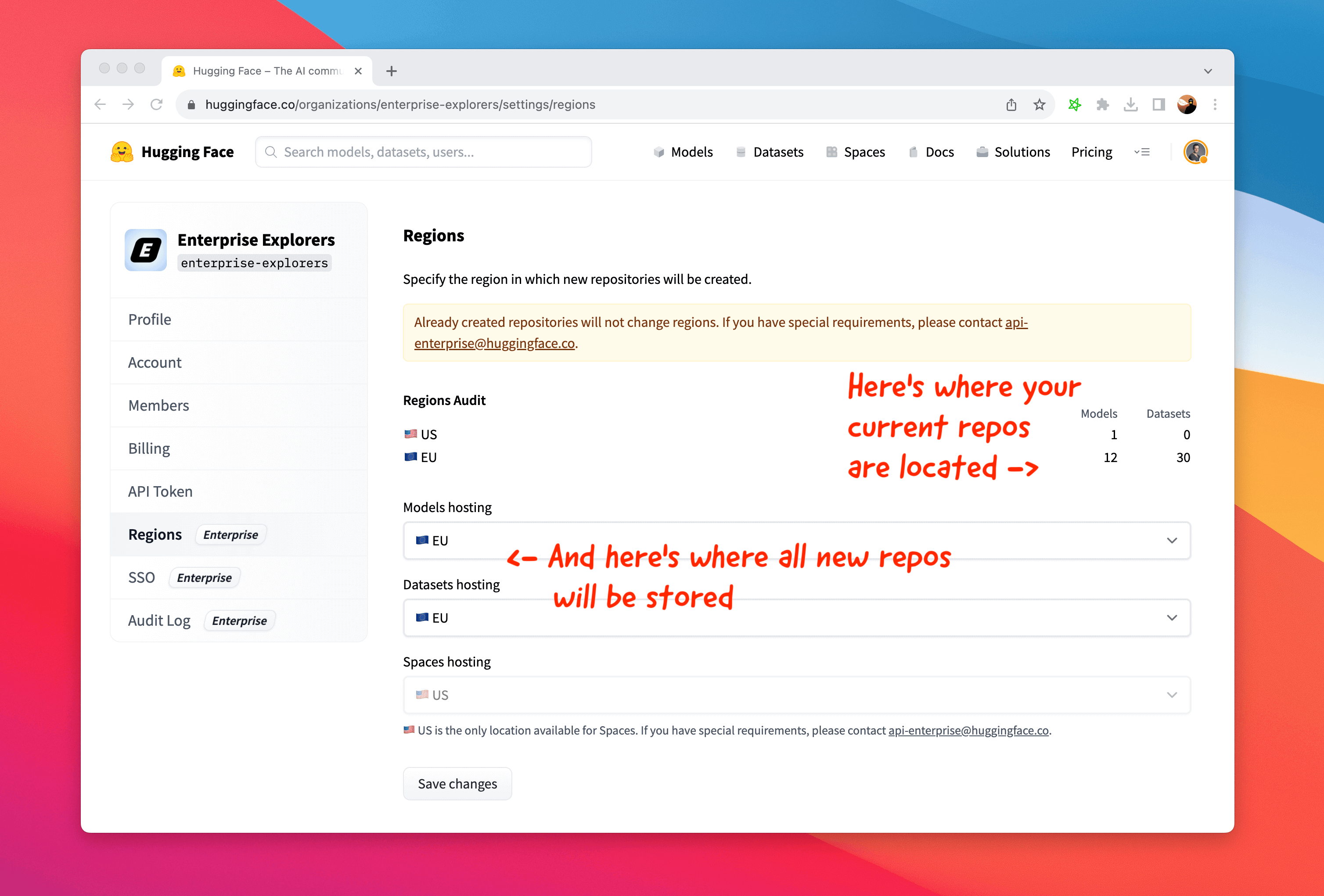 On that page you can see: - an audit of where your orgs' repos are currently located - dropdowns to select where your repos will be created ## Repository Tag Any repo (model or dataset) stored in a non-default location will display its Region directly as a tag. That way your organization's members can see at a glance where repos are located.  ## Regulatory and legal compliance In many regulated industries, you may have a requirement to store your data in a specific area. For companies in the EU, that means you can use the Hub to build ML in a GDPR compliant way: with datasets, models and inference endpoints all stored within EU data centers. If you are an Enterprise Hub customer and have further questions about this, please get in touch! ## Performance Storing your models or your datasets closer to your team and infrastructure also means significantly improved performance, for both uploads and downloads. This makes a big difference considering model weights and dataset files are usually very large.  As an example, if you are located in Europe and store your repositories in the EU region, you can expect to see ~4-5x faster upload and download speeds vs. if they were stored in the US."
"Comparing the Performance of LLMs: A Deep Dive into Roberta, Llama 2, and Mistral for Disaster Tweets Analysis with Lora",mehdiiraqui,"November 7, 2023",Lora-for-sequence-classification-with-Roberta-Llama-Mistral,"nlp, guide, llm, peft",https://huggingface.co/blog/Lora-for-sequence-classification-with-Roberta-Llama-Mistral," # Comparing the Performance of LLMs: A Deep Dive into Roberta, Llama 2, and Mistral for Disaster Tweets Analysis with Lora - [Comparing the Performance of LLMs: A Deep Dive into Roberta, Llama 2, and Mistral for Disaster Tweets Analysis with LoRA](#comparing-the-performance-of-llms-a-deep-dive-into-roberta-llama-2-and-mistral-for-disaster-tweets-analysis-with-lora) - [Introduction](#introduction) - [Hardware Used](#hardware-used) - [Goals](#goals) - [Dependencies](#dependencies) - [Pre-trained Models](#pre-trained-models) - [RoBERTa](#roberta) - [Llama 2](#llama-2) - [Mistral 7B](#mistral-7b) - [LoRA](#lora) - [Setup](#setup) - [Data preparation](#data-preparation) - [Data loading](#data-loading) - [Data Processing](#data-processing) - [Models](#models) - [RoBERTa](#roberta) - [Load RoBERTA Checkpoints for the Classification Task](#load-roberta-checkpoints-for-the-classification-task) - [LoRA setup for RoBERTa classifier](#lora-setup-for-roberta-classifier) - [Mistral](#mistral) - [Load checkpoints for the classfication model](#load-checkpoints-for-the-classfication-model) - [LoRA setup for Mistral 7B classifier](#lora-setup-for-mistral-7b-classifier) - [Llama 2](#llama-2) - [Load checkpoints for the classification mode](#load-checkpoints-for-the-classfication-mode) - [LoRA setup for Llama 2 classifier](#lora-setup-for-llama-2-classifier) - [Setup the trainer](#setup-the-trainer) - [Evaluation Metrics](#evaluation-metrics) - [Custom Trainer for Weighted Loss](#custom-trainer-for-weighted-loss) - [Trainer Setup](#trainer-setup) - [RoBERTa](#roberta) - [Mistral-7B](#mistral-7b) - [Llama 2](#llama-2) - [Hyperparameter Tuning](#hyperparameter-tuning) - [Results](#results) - [Conclusion](#conclusion) - [Resources](#resources) ## Introduction In the fast-moving world of Natural Language Processing (NLP), we often find ourselves comparing different language models to see which one works best for specific tasks. This blog post is all about comparing three models: RoBERTa, Mistral-7b, and Llama-2-7b. We used them to tackle a common problem - classifying tweets about disasters. It is important to note that Mistral and Llama 2 are large models with 7 billion parameters. In contrast, RoBERTa-large (355M parameters) is a relatively smaller model used as a baseline for the comparison study. In this blog, we used PEFT (Parameter-Efficient Fine-Tuning) technique: LoRA (Low-Rank Adaptation of Large Language Models) for fine-tuning the pre-trained model on the sequence classification task. LoRa is designed to significantly reduce the number of trainable parameters while maintaining strong downstream task performance. The main objective of this blog post is to implement LoRA fine-tuning for sequence classification tasks using three pre-trained models from Hugging Face: [meta-llama/Llama-2-7b-hf](https://huggingface.co/meta-llama/Llama-2-7b-chat-hf), [mistralai/Mistral-7B-v0.1](https://huggingface.co/mistralai/Mistral-7B-v0.1), and [roberta-large](https://huggingface.co/roberta-large) ## Hardware Used - Number of nodes: 1 - Number of GPUs per node: 1 - GPU type: A6000 - GPU memory: 48GB ## Goals - Implement fine-tuning of pre-trained LLMs using LoRA PEFT methods. - Learn how to use the HuggingFace APIs ([transformers](https://huggingface.co/docs/transformers/index), [peft](https://huggingface.co/docs/peft/index), and [datasets](https://huggingface.co/docs/datasets/index)). - Setup the hyperparameter tuning and experiment logging using [Weights & Biases](https://wandb.ai). ## Dependencies ```bash datasets evaluate peft scikit-learn torch transformers wandb ``` Note: For reproducing the reported results, please check the pinned versions in the [wandb reports](#resources). ## Pre-trained Models ### [RoBERTa](https://arxiv.org/abs/1907.11692) RoBERTa (Robustly Optimized BERT Approach) is an advanced variant of the BERT model proposed by Meta AI research team. BERT is a transformer-based language model using self-attention mechanisms for contextual word representations and trained with a masked language model objective. Note that BERT is an encoder only model used for natural language understanding tasks (such as sequence classification and token classification). RoBERTa is a popular model to fine-tune and appropriate as a baseline for our experiments. For more information, you can check the Hugging Face model [card](https://huggingface.co/docs/transformers/model_doc/roberta). ### [Llama 2](https://arxiv.org/abs/2307.09288) Llama 2 models, which stands for Large Language Model Meta AI, belong to the family of large language models (LLMs) introduced by Meta AI. The Llama 2 models vary in size, with parameter counts ranging from 7 billion to 65 billion. Llama 2 is an auto-regressive language model, based on the transformer decoder architecture. To generate text, Llama 2 processes a sequence of words as input and iteratively predicts the next token using a sliding window. Llama 2 architecture is slightly different from models like GPT-3. For instance, Llama 2 employs the SwiGLU activation function rather than ReLU and opts for rotary positional embeddings in place of absolute learnable positional embeddings. The recently released Llama 2 introduced architectural refinements to better leverage very long sequences by extending the context length to up to 4096 tokens, and using grouped-query attention (GQA) decoding. ### [Mistral 7B](https://arxiv.org/abs/2310.06825) Mistral 7B v0.1, with 7.3 billion parameters, is the first LLM introduced by Mistral AI. The main novel techniques used in Mistral 7B's architecture are: - Sliding Window Attention: Replace the full attention (square compute cost) with a sliding window based attention where each token can attend to at most 4,096 tokens from the previous layer (linear compute cost). This mechanism enables Mistral 7B to handle longer sequences, where higher layers can access historical information beyond the window size of 4,096 tokens. - Grouped-query Attention: used in Llama 2 as well, the technique optimizes the inference process (reduce processing time) by caching the key and value vectors for previously decoded tokens in the sequence. ## [LoRA](https://arxiv.org/abs/2106.09685) PEFT, Parameter Efficient Fine-Tuning, is a collection of techniques (p-tuning, prefix-tuning, IA3, Adapters, and LoRa) designed to fine-tune large models using a much smaller set of training parameters while preserving the performance levels typically achieved through full fine-tuning. LoRA, Low-Rank Adaptation, is a PEFT method that shares similarities with Adapter layers. Its primary objective is to reduce the model's trainable parameters. LoRA's operation involves learning a low rank update matrix while keeping the pre-trained weights frozen.  ## Setup RoBERTa has a limitatiom of maximum sequence length of 512, so we set the `MAX_LEN=512` for all models to ensure a fair comparison. ```python MAX_LEN = 512 roberta_checkpoint = ""roberta-large"" mistral_checkpoint = ""mistralai/Mistral-7B-v0.1"" llama_checkpoint = ""meta-llama/Llama-2-7b-hf"" ``` ## Data preparation ### Data loading We will load the dataset from Hugging Face: ```python from datasets import load_dataset dataset = load_dataset(""mehdiiraqui/twitter_disaster"") ``` Now, let's split the dataset into training and validation datasets. Then add the test set: ```python from datasets import Dataset # Split the dataset into training and validation datasets data = dataset['train'].train_test_split(train_size=0.8, seed=42) # Rename the default ""test"" split to ""validation"" data['val'] = data.pop(""test"") # Convert the test dataframe to HuggingFace dataset and add it into the first dataset data['test'] = dataset['test'] ``` Here's an overview of the dataset: ```bash DatasetDict({ train: Dataset({ features: ['id', 'keyword', 'location', 'text', 'target'], num_rows: 6090 }) val: Dataset({ features: ['id', 'keyword', 'location', 'text', 'target'], num_rows: 1523 }) test: Dataset({ features: ['id', 'keyword', 'location', 'text', 'target'], num_rows: 3263 }) }) ``` Let's check the data distribution: ```python import pandas as pd data['train'].to_pandas().info() data['test'].to_pandas().info() ``` - Train dataset ``` RangeIndex: 7613 entries, 0 to 7612 Data columns (total 5 columns): # Column Non-Null Count Dtype --- ------ -------------- ----- 0 id 7613 non-null int64 1 keyword 7552 non-null object 2 location 5080 non-null object 3 text 7613 non-null object 4 target 7613 non-null int64 dtypes: int64(2), object(3) memory usage: 297.5+ KB ``` - Test dataset ``` RangeIndex: 3263 entries, 0 to 3262 Data columns (total 5 columns): # Column Non-Null Count Dtype --- ------ -------------- ----- 0 id 3263 non-null int64 1 keyword 3237 non-null object 2 location 2158 non-null object 3 text 3263 non-null object 4 target 3263 non-null int64 dtypes: int64(2), object(3) memory usage: 127.6+ KB ``` **Target distribution in the train dataset** ``` target 0 4342 1 3271 Name: count, dtype: int64 ``` As the classes are not balanced, we will compute the positive and negative weights and use them for loss calculation later: ```python pos_weights = len(data['train'].to_pandas()) / (2 * data['train'].to_pandas().target.value_counts()[1]) neg_weights = len(data['train'].to_pandas()) / (2 * data['train'].to_pandas().target.value_counts()[0]) ``` The final weights are: ``` POS_WEIGHT, NEG_WEIGHT = (1.1637114032405993, 0.8766697374481806) ``` Then, we compute the maximum length of the column text: ```python # Number of Characters max_char = data['train'].to_pandas()['text'].str.len().max() # Number of Words max_words = data['train'].to_pandas()['text'].str.split().str.len().max() ``` ``` The maximum number of characters is 152. The maximum number of words is 31. ``` ### Data Processing Let's take a look to one row example of training data: ```python data['train'][0] ``` ``` {'id': 5285, 'keyword': 'fear', 'location': 'Thibodaux, LA', 'text': 'my worst fear. https://t.co/iH8UDz8mq3', 'target': 0} ``` The data comprises a keyword, a location and the text of the tweet. For the sake of simplicity, we select the `text` feature as the only input to the LLM. At this stage, we prepared the train, validation, and test sets in the HuggingFace format expected by the pre-trained LLMs. The next step is to define the tokenized dataset for training using the appropriate tokenizer to transform the `text` feature into two Tensors of sequence of token ids and attention masks. As each model has its specific tokenizer, we will need to define three different datasets. We start by defining the RoBERTa dataloader: - Load the tokenizer: ```python from transformers import AutoTokenizer roberta_tokenizer = AutoTokenizer.from_pretrained(roberta_checkpoint, add_prefix_space=True) ``` **Note:** The RoBERTa tokenizer has been trained to treat spaces as part of the token. As a result, the first word of the sentence is encoded differently if it is not preceded by a white space. To ensure the first word includes a space, we set `add_prefix_space=True`. Also, to maintain consistent pre-processing for all three models, we set the parameter to 'True' for Llama 2 and Mistral 7b. - Define the preprocessing function for converting one row of the dataframe: ```python def roberta_preprocessing_function(examples): return roberta_tokenizer(examples['text'], truncation=True, max_length=MAX_LEN) ``` By applying the preprocessing function to the first example of our training dataset, we have the tokenized inputs (`input_ids`) and the attention mask: ```python roberta_preprocessing_function(data['train'][0]) ``` ``` {'input_ids': [0, 127, 2373, 2490, 4, 1205, 640, 90, 4, 876, 73, 118, 725, 398, 13083, 329, 398, 119, 1343, 246, 2], 'attention_mask': [1, 1, 1, 1, 1, 1, 1, 1, 1, 1, 1, 1, 1, 1, 1, 1, 1, 1, 1, 1, 1]} ``` - Now, let's apply the preprocessing function to the entire dataset: ```python col_to_delete = ['id', 'keyword','location', 'text'] # Apply the preprocessing function and remove the undesired columns roberta_tokenized_datasets = data.map(roberta_preprocessing_function, batched=True, remove_columns=col_to_delete) # Rename the target to label as for HugginFace standards roberta_tokenized_datasets = roberta_tokenized_datasets.rename_column(""target"", ""label"") # Set to torch format roberta_tokenized_datasets.set_format(""torch"") ``` **Note:** we deleted the undesired columns from our data: id, keyword, location and text. We have deleted the text because we have already converted it into the inputs ids and the attention mask: We can have a look into our tokenized training dataset: ```python roberta_tokenized_datasets['train'][0] ``` ``` {'label': tensor(0), 'input_ids': tensor([ 0, 127, 2373, 2490, 4, 1205, 640, 90, 4, 876, 73, 118, 725, 398, 13083, 329, 398, 119, 1343, 246, 2]), 'attention_mask': tensor([1, 1, 1, 1, 1, 1, 1, 1, 1, 1, 1, 1, 1, 1, 1, 1, 1, 1, 1, 1, 1])} ``` - For generating the training batches, we also need to pad the rows of a given batch to the maximum length found in the batch. For that, we will use the `DataCollatorWithPadding` class: ```python # Data collator for padding a batch of examples to the maximum length seen in the batch from transformers import DataCollatorWithPadding roberta_data_collator = DataCollatorWithPadding(tokenizer=roberta_tokenizer) ``` You can follow the same steps for preparing the data for Mistral 7B and Llama 2 models: **Note** that Llama 2 and Mistral 7B don't have a default `pad_token_id`. So, we use the `eos_token_id` for padding as well. - Mistral 7B: ```python # Load Mistral 7B Tokenizer from transformers import AutoTokenizer, DataCollatorWithPadding mistral_tokenizer = AutoTokenizer.from_pretrained(mistral_checkpoint, add_prefix_space=True) mistral_tokenizer.pad_token_id = mistral_tokenizer.eos_token_id mistral_tokenizer.pad_token = mistral_tokenizer.eos_token def mistral_preprocessing_function(examples): return mistral_tokenizer(examples['text'], truncation=True, max_length=MAX_LEN) mistral_tokenized_datasets = data.map(mistral_preprocessing_function, batched=True, remove_columns=col_to_delete) mistral_tokenized_datasets = mistral_tokenized_datasets.rename_column(""target"", ""label"") mistral_tokenized_datasets.set_format(""torch"") # Data collator for padding a batch of examples to the maximum length seen in the batch mistral_data_collator = DataCollatorWithPadding(tokenizer=mistral_tokenizer) ``` - Llama 2: ```python # Load Llama 2 Tokenizer from transformers import AutoTokenizer, DataCollatorWithPadding llama_tokenizer = AutoTokenizer.from_pretrained(llama_checkpoint, add_prefix_space=True) llama_tokenizer.pad_token_id = llama_tokenizer.eos_token_id llama_tokenizer.pad_token = llama_tokenizer.eos_token def llama_preprocessing_function(examples): return llama_tokenizer(examples['text'], truncation=True, max_length=MAX_LEN) llama_tokenized_datasets = data.map(llama_preprocessing_function, batched=True, remove_columns=col_to_delete) llama_tokenized_datasets = llama_tokenized_datasets.rename_column(""target"", ""label"") llama_tokenized_datasets.set_format(""torch"") # Data collator for padding a batch of examples to the maximum length seen in the batch llama_data_collator = DataCollatorWithPadding(tokenizer=llama_tokenizer) ``` Now that we have prepared the tokenized datasets, the next section will showcase how to load the pre-trained LLMs checkpoints and how to set the LoRa weights. ## Models ### RoBERTa #### Load RoBERTa Checkpoints for the Classification Task We load the pre-trained RoBERTa model with a sequence classification head using the Hugging Face `AutoModelForSequenceClassification` class: ```python from transformers import AutoModelForSequenceClassification roberta_model = AutoModelForSequenceClassification.from_pretrained(roberta_checkpoint, num_labels=2) ``` #### LoRA setup for RoBERTa classifier We import LoRa configuration and set some parameters for RoBERTa classifier: - TaskType: Sequence classification - r(rank): Rank for our decomposition matrices - lora_alpha: Alpha parameter to scale the learned weights. LoRA paper advises fixing alpha at 16 - lora_dropout: Dropout probability of the LoRA layers - bias: Whether to add bias term to LoRa layers The code below uses the values recommended by the [Lora paper](https://arxiv.org/abs/2106.09685). [Later in this post](#hyperparameter-tuning) we will perform hyperparameter tuning of these parameters using `wandb`. ```python from peft import get_peft_model, LoraConfig, TaskType roberta_peft_config = LoraConfig( task_type=TaskType.SEQ_CLS, r=2, lora_alpha=16, lora_dropout=0.1, bias=""none"", ) roberta_model = get_peft_model(roberta_model, roberta_peft_config) roberta_model.print_trainable_parameters() ``` We can see that the number of trainable parameters represents only 0.64% of the RoBERTa model parameters: ```bash trainable params: 2,299,908 || all params: 356,610,052 || trainable%: 0.6449363911929212 ``` ### Mistral #### Load checkpoints for the classfication model Let's load the pre-trained Mistral-7B model with a sequence classification head: ```python from transformers import AutoModelForSequenceClassification import torch mistral_model = AutoModelForSequenceClassification.from_pretrained( pretrained_model_name_or_path=mistral_checkpoint, num_labels=2, device_map=""auto"" ) ``` For Mistral 7B, we have to add the padding token id as it is not defined by default. ```python mistral_model.config.pad_token_id = mistral_model.config.eos_token_id ``` #### LoRa setup for Mistral 7B classifier For Mistral 7B model, we need to specify the `target_modules` (the query and value vectors from the attention modules): ```python from peft import get_peft_model, LoraConfig, TaskType mistral_peft_config = LoraConfig( task_type=TaskType.SEQ_CLS, r=2, lora_alpha=16, lora_dropout=0.1, bias=""none"", target_modules=[ ""q_proj"", ""v_proj"", ], ) mistral_model = get_peft_model(mistral_model, mistral_peft_config) mistral_model.print_trainable_parameters() ``` The number of trainable parameters reprents only 0.024% of the Mistral model parameters: ``` trainable params: 1,720,320 || all params: 7,112,380,416 || trainable%: 0.02418768259540745 ``` ### Llama 2 #### Load checkpoints for the classfication mode Let's load pre-trained Llama 2 model with a sequence classification header. ```python from transformers import AutoModelForSequenceClassification import torch llama_model = AutoModelForSequenceClassification.from_pretrained( pretrained_model_name_or_path=llama_checkpoint, num_labels=2, device_map=""auto"", offload_folder=""offload"", trust_remote_code=True ) ``` For Llama 2, we have to add the padding token id as it is not defined by default. ```python llama_model.config.pad_token_id = llama_model.config.eos_token_id ``` #### LoRa setup for Llama 2 classifier We define LoRa for Llama 2 with the same parameters as for Mistral: ```python from peft import get_peft_model, LoraConfig, TaskType llama_peft_config = LoraConfig( task_type=TaskType.SEQ_CLS, r=16, lora_alpha=16, lora_dropout=0.05, bias=""none"", target_modules=[ ""q_proj"", ""v_proj"", ], ) llama_model = get_peft_model(llama_model, llama_peft_config) llama_model.print_trainable_parameters() ``` The number of trainable parameters reprents only 0.12% of the Llama 2 model parameters: ``` trainable params: 8,404,992 || all params: 6,615,748,608 || trainable%: 0.1270452143516515 ``` At this point, we defined the tokenized dataset for training as well as the LLMs setup with LoRa layers. The following section will introduce how to launch training using the HuggingFace `Trainer` class. ## Setup the trainer ### Evaluation Metrics First, we define the performance metrics we will use to compare the three models: F1 score, recall, precision and accuracy: ```python import evaluate import numpy as np def compute_metrics(eval_pred): # All metrics are already predefined in the HF `evaluate` package precision_metric = evaluate.load(""precision"") recall_metric = evaluate.load(""recall"") f1_metric= evaluate.load(""f1"") accuracy_metric = evaluate.load(""accuracy"") logits, labels = eval_pred # eval_pred is the tuple of predictions and labels returned by the model predictions = np.argmax(logits, axis=-1) precision = precision_metric.compute(predictions=predictions, references=labels)[""precision""] recall = recall_metric.compute(predictions=predictions, references=labels)[""recall""] f1 = f1_metric.compute(predictions=predictions, references=labels)[""f1""] accuracy = accuracy_metric.compute(predictions=predictions, references=labels)[""accuracy""] # The trainer is expecting a dictionary where the keys are the metrics names and the values are the scores. return {""precision"": precision, ""recall"": recall, ""f1-score"": f1, 'accuracy': accuracy} ``` ### Custom Trainer for Weighted Loss As mentioned at the beginning of this post, we have an imbalanced distribution between positive and negative classes. We need to train our models with a weighted cross-entropy loss to account for that. The `Trainer` class doesn't support providing a custom loss as it expects to get the loss directly from the model's outputs. So, we need to define our custom `WeightedCELossTrainer` that overrides the `compute_loss` method to calculate the weighted cross-entropy loss based on the model's predictions and the input labels: ```python from transformers import Trainer class WeightedCELossTrainer(Trainer): def compute_loss(self, model, inputs, return_outputs=False): labels = inputs.pop(""labels"") # Get model's predictions outputs = model(**inputs) logits = outputs.get(""logits"") # Compute custom loss loss_fct = torch.nn.CrossEntropyLoss(weight=torch.tensor([neg_weights, pos_weights], device=model.device, dtype=logits.dtype)) loss = loss_fct(logits.view(-1, self.model.config.num_labels), labels.view(-1)) return (loss, outputs) if return_outputs else loss ``` ### Trainer Setup Let's set the training arguments and the trainer for the three models. #### RoBERTa First important step is to move the models to the GPU device for training. ```python roberta_model = roberta_model.cuda() roberta_model.device() ``` It will print the following: ``` device(type='cuda', index=0) ``` Then, we set the training arguments: ```python from transformers import TrainingArguments lr = 1e-4 batch_size = 8 num_epochs = 5 training_args = TrainingArguments( output_dir=""roberta-large-lora-token-classification"", learning_rate=lr, lr_scheduler_type= ""constant"", warmup_ratio= 0.1, max_grad_norm= 0.3, per_device_train_batch_size=batch_size, per_device_eval_batch_size=batch_size, num_train_epochs=num_epochs, weight_decay=0.001, evaluation_strategy=""epoch"", save_strategy=""epoch"", load_best_model_at_end=True, report_to=""wandb"", fp16=False, gradient_checkpointing=True, ) ``` Finally, we define the RoBERTa trainer by providing the model, the training arguments and the tokenized datasets: ```python roberta_trainer = WeightedCELossTrainer( model=roberta_model, args=training_args, train_dataset=roberta_tokenized_datasets['train'], eval_dataset=roberta_tokenized_datasets[""val""], data_collator=roberta_data_collator, compute_metrics=compute_metrics ) ``` #### Mistral-7B Similar to RoBERTa, we initialize the `WeightedCELossTrainer` as follows: ```python from transformers import TrainingArguments, Trainer mistral_model = mistral_model.cuda() lr = 1e-4 batch_size = 8 num_epochs = 5 training_args = TrainingArguments( output_dir=""mistral-lora-token-classification"", learning_rate=lr, lr_scheduler_type= ""constant"", warmup_ratio= 0.1, max_grad_norm= 0.3, per_device_train_batch_size=batch_size, per_device_eval_batch_size=batch_size, num_train_epochs=num_epochs, weight_decay=0.001, evaluation_strategy=""epoch"", save_strategy=""epoch"", load_best_model_at_end=True, report_to=""wandb"", fp16=True, gradient_checkpointing=True, ) mistral_trainer = WeightedCELossTrainer( model=mistral_model, args=training_args, train_dataset=mistral_tokenized_datasets['train'], eval_dataset=mistral_tokenized_datasets[""val""], data_collator=mistral_data_collator, compute_metrics=compute_metrics ) ``` **Note** that we needed to enable half-precision training by setting `fp16` to `True`. The main reason is that Mistral-7B is large, and its weights cannot fit into one GPU memory (48GB) with full float32 precision. #### Llama 2 Similar to Mistral 7B, we define the trainer as follows: ```python from transformers import TrainingArguments, Trainer llama_model = llama_model.cuda() lr = 1e-4 batch_size = 8 num_epochs = 5 training_args = TrainingArguments( output_dir=""llama-lora-token-classification"", learning_rate=lr, lr_scheduler_type= ""constant"", warmup_ratio= 0.1, max_grad_norm= 0.3, per_device_train_batch_size=batch_size, per_device_eval_batch_size=batch_size, num_train_epochs=num_epochs, weight_decay=0.001, evaluation_strategy=""epoch"", save_strategy=""epoch"", load_best_model_at_end=True, report_to=""wandb"", fp16=True, gradient_checkpointing=True, ) llama_trainer = WeightedCELossTrainer( model=llama_model, args=training_args, train_dataset=llama_tokenized_datasets['train'], eval_dataset=llama_tokenized_datasets[""val""], data_collator=llama_data_collator, compute_metrics=compute_metrics ) ``` ## Hyperparameter Tuning We have used Wandb Sweep API to run hyperparameter tunning with Bayesian search strategy (30 runs). The hyperparameters tuned are the following. | method | metric | lora_alpha | lora_bias | lora_dropout | lora_rank | lr | max_length | |--------|---------------------|-------------------------------------------|---------------------------|-------------------------|----------------------------------------------------|-----------------------------|---------------------------| | bayes | goal: maximize | distribution: categorical | distribution: categorical | distribution: uniform | distribution: categorical | distribution: uniform | distribution: categorical | | | name: eval/f1-score | values:
-16
-32
-64 | values: None | -max: 0.1
-min: 0 | values:
-4
-8
-16
-32 | -max: 2e-04
-min: 1e-05 | values: 512 | | For more information, you can check the Wandb experiment report in the [resources sections](#resources). ## Results | Models | F1 score | Training time | Memory consumption | Number of trainable parameters | |---------|----------|----------------|------------------------------|--------------------------------| | RoBERTa | 0.8077 | 538 seconds | GPU1: 9.1 Gb
GPU2: 8.3 Gb | 0.64% | | Mistral 7B | 0.7364 | 2030 seconds | GPU1: 29.6 Gb
GPU2: 29.5 Gb | 0.024% | | Llama 2 | 0.7638 | 2052 seconds | GPU1: 35 Gb
GPU2: 33.9 Gb | 0.12% | ## Conclusion In this blog post, we compared the performance of three large language models (LLMs) - RoBERTa, Mistral 7b, and Llama 2 - for disaster tweet classification using LoRa. From the performance results, we can see that RoBERTa is outperforming Mistral 7B and Llama 2 by a large margin. This raises the question about whether we really need a complex and large LLM for tasks like short-sequence binary classification? One learning we can draw from this study is that one should account for the specific project requirements, available resources, and performance needs to choose the LLMs model to use. Also, for relatively *simple* prediction tasks with short sequences base models such as RoBERTa remain competitive. Finally, we showcase that LoRa method can be applied to both encoder (RoBERTa) and decoder (Llama 2 and Mistral 7B) models. ## Resources 1. You can find the code script in the following [Github project](https://github.com/mehdiir/Roberta-Llama-Mistral/). 2. You can check the hyper-param search results in the following Weight&Bias reports: - [RoBERTa](https://api.wandb.ai/links/mehdi-iraqui/505c22j1) - [Mistral 7B](https://api.wandb.ai/links/mehdi-iraqui/24vveyxp) - [Llama 2](https://api.wandb.ai/links/mehdi-iraqui/qq8beod0)"
Introducing Prodigy-HF: a direct integration with Hugging Face,koaning,"November 7, 2023",prodigy-hf,"community, nlp, datasets, guide",https://huggingface.co/blog/prodigy-hf," # Introducing Prodigy-HF [Prodigy](https://prodi.gy/) is an annotation tool made by [Explosion](https://explosion.ai/), a company well known as the creators of [spaCy](https://spacy.io/). It's a fully scriptable product with a large community around it. The product has many features, including tight integration with spaCy and active learning capabilities. But the main feature of the product is that it is programmatically customizable with Python. To foster this customisability, Explosion has started releasing [plugins](https://prodi.gy/docs/plugins). These plugins integrate with third-party tools in an open way that encourages users to work on bespoke annotation workflows. However, one customization specifically deserves to be celebrated explicitly. Last week, Explosion introduced [Prodigy-HF](https://github.com/explosion/prodigy-hf), which offers code recipes that directly integrate with the Hugging Face stack. It's been a much-requested feature on the [Prodigy support forum](https://support.prodi.gy/), so we're super excited to have it out there. ## Features The first main feature is that this plugin allows you to train and re-use Hugging Face models on your annotated data. That means if you've been annotating data in our interface for named entity recognition, you can directly fine-tune BERT models against it. What the Prodigy NER interface looks like. After installing the plugin you can call the `hf.train.ner` recipe from the command line to train a transformer model directly on your own data. ``` python -m prodigy hf.train.ner fashion-train,eval:fashion-eval path/to/model-out --model ""distilbert-base-uncased"" ``` This will fine-tune the `distilbert-base-uncased` model for the dataset you've stored in Prodigy and save it to disk. Similarly, this plugin also supports models for text classification via a very similar interface. ``` python -m prodigy hf.train.textcat fashion-train,eval:fashion-eval path/to/model-out --model ""distilbert-base-uncased"" ``` This offers a lot of flexibility because the tool directly integrates with the `AutoTokenizer` and `AutoModel` classes of Hugging Face transformers. Any transformer model on the hub can be fine-tuned on your own dataset with just a single command. These models will be serialised on disk, which means that you can upload them to the Hugging Face Hub, or re-use them to help you annotate data. This can save a lot of time, especially for NER tasks. To re-use a trained NER model you can use the `hf.correct.ner` recipe. ``` python -m prodigy hf.correct.ner fashion-train path/to/model-out examples.jsonl ``` This will give you a similar interface as before, but now the model predictions will be shown in the interface as well. ### Upload The second feature, which is equally exciting, is that you can now also publish your annotated datasets on the Hugging Face Hub. This is great if you're interested in sharing datasets that others would like to use. ``` python -m prodigy hf.upload / ``` We're particularly fond of this upload feature because it encourages collaboration. People can annotate their own datasets independently of each other, but still benefit when they share the data with the wider community. ## More to come We hope that this direct integration with the Hugging Face ecosystem enables many users to experiment more. The Hugging Face Hub offers _many_ [models](https://huggingface.co/models) for a wide array of tasks as well as a wide array of languages. We really hope that this integration makes it easier to get data annotated, even if you've got a more domain specific and experimental use-case. More features for this library are on their way, and feel free to reach out on the [Prodigy forum](https://support.prodi.gy/) if you have more questions. We'd also like to thank the team over at Hugging Face for their feedback on this plugin, specifically @davanstrien, who suggested to add the upload feature. Thanks! "
Make your llama generation time fly with AWS Inferentia2,dacorvo,"November 7, 2023",inferentia-llama2,"guide, text-generation, llama2, aws",https://huggingface.co/blog/inferentia-llama2," # Make your llama generation time fly with AWS Inferentia2 In a [previous post on the Hugging Face blog](https://huggingface.co/blog/accelerate-transformers-with-inferentia2), we introduced [AWS Inferentia2](https://aws.amazon.com/ec2/instance-types/inf2/), the second-generation AWS Inferentia accelerator, and explained how you could use [optimum-neuron](https://huggingface.co/docs/optimum-neuron/index) to quickly deploy Hugging Face models for standard text and vision tasks on AWS Inferencia 2 instances. In a further step of integration with the [AWS Neuron SDK](https://github.com/aws-neuron/aws-neuron-sdk), it is now possible to use 🤗 [optimum-neuron](https://huggingface.co/docs/optimum-neuron/index) to deploy LLM models for text generation on AWS Inferentia2. And what better model could we choose for that demonstration than [Llama 2](https://huggingface.co/meta-llama/Llama-2-13b-hf), one of the most popular models on the [Hugging Face hub](https://huggingface.co/models). ## Setup 🤗 optimum-neuron on your Inferentia2 instance Our recommendation is to use the [Hugging Face Neuron Deep Learning AMI](https://aws.amazon.com/marketplace/pp/prodview-gr3e6yiscria2) (DLAMI). The DLAMI comes with all required libraries pre-packaged for you, including the Optimum Neuron, Neuron Drivers, Transformers, Datasets, and Accelerate. Alternatively, you can use the [Hugging Face Neuron SDK DLC](https://github.com/aws/deep-learning-containers/releases?q=hf&expanded=true) to deploy on Amazon SageMaker. *Note: stay tuned for an upcoming post dedicated to SageMaker deployment.* Finally, these components can also be installed manually on a fresh Inferentia2 instance following the `optimum-neuron` [installation instructions](https://huggingface.co/docs/optimum-neuron/installation). ## Export the Llama 2 model to Neuron As explained in the [optimum-neuron documentation](https://huggingface.co/docs/optimum-neuron/guides/export_model#why-compile-to-neuron-model), models need to be compiled and exported to a serialized format before running them on Neuron devices. Fortunately, 🤗 `optimum-neuron` offers a [very simple API](https://huggingface.co/docs/optimum-neuron/guides/models#configuring-the-export-of-a-generative-model) to export standard 🤗 [transformers models](https://huggingface.co/docs/transformers/index) to the Neuron format. ``` >>> from optimum.neuron import NeuronModelForCausalLM >>> compiler_args = {""num_cores"": 24, ""auto_cast_type"": 'fp16'} >>> input_shapes = {""batch_size"": 1, ""sequence_length"": 2048} >>> model = NeuronModelForCausalLM.from_pretrained( ""meta-llama/Llama-2-7b-hf"", export=True, **compiler_args, **input_shapes) ``` This deserves a little explanation: - using `compiler_args`, we specify on how many cores we want the model to be deployed (each neuron device has two cores), and with which precision (here `float16`), - using `input_shape`, we set the static input and output dimensions of the model. All model compilers require static shapes, and neuron makes no exception. Note that the `sequence_length` not only constrains the length of the input context, but also the length of the KV cache, and thus, the output length. Depending on your choice of parameters and inferentia host, this may take from a few minutes to more than an hour. Fortunately, you will need to do this only once because you can save your model and reload it later. ``` >>> model.save_pretrained(""a_local_path_for_compiled_neuron_model"") ``` Even better, you can push it to the [Hugging Face hub](https://huggingface.co/models). ``` >>> model.push_to_hub( ""a_local_path_for_compiled_neuron_model"", repository_id=""aws-neuron/Llama-2-7b-hf-neuron-latency"") ``` ## Generate Text using Llama 2 on AWS Inferentia2 Once your model has been exported, you can generate text using the transformers library, as it has been described in [detail in this previous post](https://huggingface.co/blog/how-to-generate). ``` >>> from optimum.neuron import NeuronModelForCausalLM >>> from transformers import AutoTokenizer >>> model = NeuronModelForCausalLM.from_pretrained('aws-neuron/Llama-2-7b-hf-neuron-latency') >>> tokenizer = AutoTokenizer.from_pretrained(""aws-neuron/Llama-2-7b-hf-neuron-latency"") >>> inputs = tokenizer(""What is deep-learning ?"", return_tensors=""pt"") >>> outputs = model.generate(**inputs, max_new_tokens=128, do_sample=True, temperature=0.9, top_k=50, top_p=0.9) >>> tokenizer.batch_decode(outputs, skip_special_tokens=True) ['What is deep-learning ?\nThe term “deep-learning” refers to a type of machine-learning that aims to model high-level abstractions of the data in the form of a hierarchy of multiple layers of increasingly complex processing nodes.'] ``` *Note: when passing multiple input prompts to a model, the resulting token sequences must be padded to the left with an end-of-stream token. The tokenizers saved with the exported models are configured accordingly.* The following generation strategies are supported: - greedy search, - multinomial sampling with top-k and top-p (with temperature). Most logits pre-processing/filters (such as repetition penalty) are supported. ## All-in-one with optimum-neuron pipelines For those who like to keep it simple, there is an even simpler way to use an LLM model on AWS inferentia 2 using [optimum-neuron pipelines](https://huggingface.co/docs/optimum-neuron/guides/pipelines). Using them is as simple as: ``` >>> from optimum.neuron import pipeline >>> p = pipeline('text-generation', 'aws-neuron/Llama-2-7b-hf-neuron-budget') >>> p(""My favorite place on earth is"", max_new_tokens=64, do_sample=True, top_k=50) [{'generated_text': 'My favorite place on earth is the ocean. It is where I feel most at peace. I love to travel and see new places. I have a'}] ``` ## Benchmarks But how much efficient is text-generation on Inferentia2? Let's figure out! We have uploaded on the hub pre-compiled versions of the LLama 2 7B and 13B models with different configurations: | Model type | num cores | batch_size | Hugging Face Hub model | |----------------------------|-----------|------------|-------------------------------------------| | Llama2 7B - B (budget) | 2 | 1 |[aws-neuron/Llama-2-7b-hf-neuron-budget](https://huggingface.co/aws-neuron/Llama-2-7b-hf-neuron-budget) | | Llama2 7B - L (latency) | 24 | 1 |[aws-neuron/Llama-2-7b-hf-neuron-latency](https://huggingface.co/aws-neuron/Llama-2-7b-hf-neuron-latency) | | Llama2 7B - T (throughput) | 24 | 4 |[aws-neuron/Llama-2-7b-hf-neuron-throughput](https://huggingface.co/aws-neuron/Llama-2-7b-hf-neuron-throughput) | | Llama2 13B - L (latency) | 24 | 1 |[aws-neuron/Llama-2-13b-hf-neuron-latency](https://huggingface.co/aws-neuron/Llama-2-13b-hf-neuron-latency) | | Llama2 13B - T (throughput)| 24 | 4 |[aws-neuron/Llama-2-13b-hf-neuron-throughput](https://huggingface.co/aws-neuron/Llama-2-13b-hf-neuron-throughput)| *Note: all models are compiled with a maximum sequence length of 2048.* The `llama2 7B` ""budget"" model is meant to be deployed on `inf2.xlarge` instance that has only one neuron device, and enough `cpu` memory to load the model. All other models are compiled to use the full extent of cores available on the `inf2.48xlarge` instance. *Note: please refer to the [inferentia2 product page](https://aws.amazon.com/ec2/instance-types/inf2/) for details on the available instances.* We created two ""latency"" oriented configurations for the `llama2 7B` and `llama2 13B` models that can serve only one request at a time, but at full speed. We also created two ""throughput"" oriented configurations to serve up to four requests in parallel. To evaluate the models, we generate tokens up to a total sequence length of 1024, starting from 256 input tokens (i.e. we generate 256, 512 and 768 tokens). *Note: the ""budget"" model numbers are reported but not included in the graphs for better readability.* ### Encoding time The encoding time is the time required to process the input tokens and generate the first output token. It is a very important metric, as it corresponds to the latency directly perceived by the user when streaming generated tokens. We test the encoding time for increasing context sizes, 256 input tokens corresponding roughly to a typical Q/A usage, while 768 is more typical of a Retrieval Augmented Generation (RAG) use-case. The ""budget"" model (`Llama2 7B-B`) is deployed on an `inf2.xlarge` instance while other models are deployed on an `inf2.48xlarge` instance. Encoding time is expressed in **seconds**. | input tokens | Llama2 7B-L | Llama2 7B-T | Llama2 13B-L | Llama2 13B-T | Llama2 7B-B | |-----------------|----------------|----------------|-----------------|-----------------|----------------| | 256 | 0.5 | 0.9 | 0.6 | 1.8 | 0.3 | | 512 | 0.7 | 1.6 | 1.1 | 3.0 | 0.4 | | 768 | 1.1 | 3.3 | 1.7 | 5.2 | 0.5 |  We can see that all deployed models exhibit excellent response times, even for long contexts. ### End-to-end Latency The end-to-end latency corresponds to the total time to reach a sequence length of 1024 tokens. It therefore includes the encoding and generation time. The ""budget"" model (`Llama2 7B-B`) is deployed on an `inf2.xlarge` instance while other models are deployed on an `inf2.48xlarge` instance. Latency is expressed in **seconds**. | new tokens | Llama2 7B-L | Llama2 7B-T | Llama2 13B-L | Llama2 13B-T | Llama2 7B-B | |---------------|----------------|----------------|-----------------|-----------------|----------------| | 256 | 2.3 | 2.7 | 3.5 | 4.1 | 15.9 | | 512 | 4.4 | 5.3 | 6.9 | 7.8 | 31.7 | | 768 | 6.2 | 7.7 | 10.2 | 11.1 | 47.3 |  All models deployed on the high-end instance exhibit a good latency, even those actually configured to optimize throughput. The ""budget"" deployed model latency is significantly higher, but still ok. ### Throughput We adopt the same convention as other benchmarks to evaluate the throughput, by dividing the end-to-end latency by the sum of both input and output tokens. In other words, we divide the end-to-end latency by `batch_size * sequence_length` to obtain the number of generated tokens per second. The ""budget"" model (`Llama2 7B-B`) is deployed on an `inf2.xlarge` instance while other models are deployed on an `inf2.48xlarge` instance. Throughput is expressed in **tokens/second**. | new tokens | Llama2 7B-L | Llama2 7B-T | Llama2 13B-L | Llama2 13B-T | Llama2 7B-B | |---------------|----------------|----------------|-----------------|-----------------|----------------| | 256 | 227 | 750 | 145 | 504 | 32 | | 512 | 177 | 579 | 111 | 394 | 24 | | 768 | 164 | 529 | 101 | 370 | 22 |  Again, the models deployed on the high-end instance have a very good throughput, even those optimized for latency. The ""budget"" model has a much lower throughput, but still ok for a streaming use-case, considering that an average reader reads around 5 words per-second. ## Conclusion We have illustrated how easy it is to deploy `llama2` models from the [Hugging Face hub](https://huggingface.co/models) on [AWS Inferentia2](https://aws.amazon.com/ec2/instance-types/inf2/) using 🤗 [optimum-neuron](https://huggingface.co/docs/optimum-neuron/index). The deployed models demonstrate very good performance in terms of encoding time, latency and throughput. Interestingly, the deployed models latency is not too sensitive to the batch size, which opens the way for their deployment on inference endpoints serving multiple requests in parallel. There is still plenty of room for improvement though: - in the current implementation, the only way to augment the throughput is to increase the batch size, but it is currently limited by the device memory. Alternative options such as pipelining are currently integrated, - the static sequence length limits the model ability to encode long contexts. It would be interesting to see if attention sinks might be a valid option to address this."
SDXL in 4 steps with Latent Consistency LoRAs,pcuenq,"November 9, 2023",lcm_lora,"sdxl, lcm, stable diffusion, guide",https://huggingface.co/blog/lcm_lora," # SDXL in 4 steps with Latent Consistency LoRAs [Latent Consistency Models (LCM)](https://huggingface.co/papers/2310.04378) are a way to decrease the number of steps required to generate an image with Stable Diffusion (or SDXL) by _distilling_ the original model into another version that requires fewer steps (4 to 8 instead of the original 25 to 50). Distillation is a type of training procedure that attempts to replicate the outputs from a source model using a new one. The distilled model may be designed to be smaller (that’s the case of [DistilBERT](https://huggingface.co/docs/transformers/model_doc/distilbert) or the recently-released [Distil-Whisper](https://github.com/huggingface/distil-whisper)) or, in this case, require fewer steps to run. It’s usually a lengthy and costly process that requires huge amounts of data, patience, and a few GPUs. Well, that was the status quo before today! We are delighted to announce a new method that can essentially make Stable Diffusion and SDXL faster, as if they had been distilled using the LCM process! How does it sound to run _any_ SDXL model in about 1 second instead of 7 on a 3090, or 10x faster on Mac? Read on for details! ## Contents - [Method Overview](#method-overview) - [Why does this matter](#why-does-this-matter) - [Fast Inference with SDXL LCM LoRAs](#fast-inference-with-sdxl-lcm-loras) - [Quality Comparison](#quality-comparison) - [Guidance Scale and Negative Prompts](#guidance-scale-and-negative-prompts) - [Quality vs base SDXL](#quality-vs-base-sdxl) - [LCM LoRAs with other Models](#lcm-loras-with-other-models) - [Full Diffusers Integration](#full-diffusers-integration) - [Benchmarks](#benchmarks) - [LCM LoRAs and Models Released Today](#lcm-loras-and-models-released-today) - [Bonus: Combine LCM LoRAs with regular SDXL LoRAs](#bonus-combine-lcm-loras-with-regular-sdxl-loras) - [How to train LCM LoRAs](#how-to-train-lcm-loras) - [Resources](#resources) - [Credits](#credits) ## Method Overview So, what’s the trick? For latent consistency distillation, each model needs to be distilled separately. The core idea with LCM LoRA is to train just a small number of adapters, [known as LoRA layers](https://huggingface.co/docs/peft/conceptual_guides/lora), instead of the full model. The resulting LoRAs can then be applied to any fine-tuned version of the model without having to distil them separately. If you are itching to see how this looks in practice, just jump to the [next section](#fast-inference-with-sdxl-lcm-loras) to play with the inference code. If you want to train your own LoRAs, this is the process you’d use: 1. Select an available teacher model from the Hub. For example, you can use [SDXL (base)](https://huggingface.co/stabilityai/stable-diffusion-xl-base-1.0), or any fine-tuned or dreamboothed version you like. 2. [Train a LCM LoRA](#how-to-train-lcm-models-and-loras) on the model. LoRA is a type of performance-efficient fine-tuning, or PEFT, that is much cheaper to accomplish than full model fine-tuning. For additional details on PEFT, please check [this blog post](https://huggingface.co/blog/peft) or [the diffusers LoRA documentation](https://huggingface.co/docs/diffusers/training/lora). 3. Use the LoRA with any SDXL diffusion model and the LCM scheduler; bingo! You get high-quality inference in just a few steps. For more details on the process, please [download our paper](https://huggingface.co/latent-consistency/lcm-lora-sdxl/resolve/main/LCM-LoRA-Technical-Report.pdf). ## Why does this matter? Fast inference of Stable Diffusion and SDXL enables new use-cases and workflows. To name a few: - **Accessibility**: generative tools can be used effectively by more people, even if they don’t have access to the latest hardware. - **Faster iteration**: get more images and multiple variants in a fraction of the time! This is great for artists and researchers; whether for personal or commercial use. - Production workloads may be possible on different accelerators, including CPUs. - Cheaper image generation services. To gauge the speed difference we are talking about, generating a single 1024x1024 image on an M1 Mac with SDXL (base) takes about a minute. Using the LCM LoRA, we get great results in just ~6s (4 steps). This is an order of magnitude faster, and not having to wait for results is a game-changer. Using a 4090, we get almost instant response (less than 1s). This unlocks the use of SDXL in applications where real-time events are a requirement. ## Fast Inference with SDXL LCM LoRAs The version of `diffusers` released today makes it very easy to use LCM LoRAs: ```py from diffusers import DiffusionPipeline, LCMScheduler import torch model_id = ""stabilityai/stable-diffusion-xl-base-1.0"" lcm_lora_id = ""latent-consistency/lcm-lora-sdxl"" pipe = DiffusionPipeline.from_pretrained(model_id, variant=""fp16"") pipe.load_lora_weights(lcm_lora_id) pipe.scheduler = LCMScheduler.from_config(pipe.scheduler.config) pipe.to(device=""cuda"", dtype=torch.float16) prompt = ""close-up photography of old man standing in the rain at night, in a street lit by lamps, leica 35mm summilux"" images = pipe( prompt=prompt, num_inference_steps=4, guidance_scale=1, ).images[0] ``` Note how the code: - Instantiates a standard diffusion pipeline with the SDXL 1.0 base model. - Applies the LCM LoRA. - Changes the scheduler to the LCMScheduler, which is the one used in latent consistency models. - That’s it! This would result in the following full-resolution image: ![]()
Image generated with SDXL in 4 steps using an LCM LoRA.
### Quality Comparison Let’s see how the number of steps impacts generation quality. The following code will generate images with 1 to 8 total inference steps: ```py images = [] for steps in range(8): generator = torch.Generator(device=pipe.device).manual_seed(1337) image = pipe( prompt=prompt, num_inference_steps=steps+1, guidance_scale=1, generator=generator, ).images[0] images.append(image) ``` These are the 8 images displayed in a grid: ![]()
LCM LoRA generations with 1 to 8 steps.
As expected, using just **1** step produces an approximate shape without discernible features and lacking texture. However, results quickly improve, and they are usually very satisfactory in just 4 to 6 steps. Personally, I find the 8-step image in the previous test to be a bit too saturated and “cartoony” for my taste, so I’d probably choose between the ones with 5 and 6 steps in this example. Generation is so fast that you can create a bunch of different variants using just 4 steps, and then select the ones you like and iterate using a couple more steps and refined prompts as necessary. ### Guidance Scale and Negative Prompts Note that in the previous examples we used a `guidance_scale` of `1`, which effectively disables it. This works well for most prompts, and it’s fastest, but ignores negative prompts. You can also explore using negative prompts by providing a guidance scale between `1` and `2` – we found that larger values don’t work. ### Quality vs base SDXL How does this compare against the standard SDXL pipeline, in terms of quality? Let’s see an example! We can quickly revert our pipeline to a standard SDXL pipeline by unloading the LoRA weights and switching to the default scheduler: ```py from diffusers import EulerDiscreteScheduler pipe.unload_lora_weights() pipe.scheduler = EulerDiscreteScheduler.from_config(pipe.scheduler.config) ``` Then we can run inference as usual for SDXL. We’ll gather results using varying number of steps: ```py images = [] for steps in (1, 4, 8, 15, 20, 25, 30, 50): generator = torch.Generator(device=pipe.device).manual_seed(1337) image = pipe( prompt=prompt, num_inference_steps=steps, generator=generator, ).images[0] images.append(image) ``` ![]()
SDXL pipeline results (same prompt and random seed), using 1, 4, 8, 15, 20, 25, 30, and 50 steps.
As you can see, images in this example are pretty much useless until ~20 steps (second row), and quality still increases niteceably with more steps. The details in the final image are amazing, but it took 50 steps to get there. ### LCM LoRAs with other models This technique also works for any other fine-tuned SDXL or Stable Diffusion model. To demonstrate, let's see how to run inference on [`collage-diffusion`](https://huggingface.co/wavymulder/collage-diffusion), a model fine-tuned from [Stable Diffusion v1.5](https://huggingface.co/runwayml/stable-diffusion-v1-5) using Dreambooth. The code is similar to the one we saw in the previous examples. We load the fine-tuned model, and then the LCM LoRA suitable for Stable Diffusion v1.5. ```py from diffusers import DiffusionPipeline, LCMScheduler import torch model_id = ""wavymulder/collage-diffusion"" lcm_lora_id = ""latent-consistency/lcm-lora-sdv1-5"" pipe = DiffusionPipeline.from_pretrained(model_id, variant=""fp16"") pipe.scheduler = LCMScheduler.from_config(pipe.scheduler.config) pipe.load_lora_weights(lcm_lora_id) pipe.to(device=""cuda"", dtype=torch.float16) prompt = ""collage style kid sits looking at the night sky, full of stars"" generator = torch.Generator(device=pipe.device).manual_seed(1337) images = pipe( prompt=prompt, generator=generator, negative_prompt=negative_prompt, num_inference_steps=4, guidance_scale=1, ).images[0] images ``` ![]()
LCM LoRA technique with a Dreambooth Stable Diffusion v1.5 model, allowing 4-step inference.
### Full Diffusers Integration The integration of LCM in `diffusers` makes it possible to take advantage of many features and workflows that are part of the diffusers toolbox. For example: - Out of the box `mps` support for Macs with Apple Silicon. - Memory and performance optimizations like flash attention or `torch.compile()`. - Additional memory saving strategies for low-RAM environments, including model offload. - Workflows like ControlNet or image-to-image. - Training and fine-tuning scripts. ## Benchmarks This section is not meant to be exhaustive, but illustrative of the generation speed we achieve on various computers. Let us stress again how liberating it is to explore image generation so easily. | Hardware | SDXL LoRA LCM (4 steps) | SDXL standard (25 steps) | |----------------------------------------|-------------------------|--------------------------| | Mac, M1 Max | 6.5s | 64s | | 2080 Ti | 4.7s | 10.2s | | 3090 | 1.4s | 7s | | 4090 | 0.7s | 3.4s | | T4 (Google Colab Free Tier) | 8.4s | 26.5s | | A100 (80 GB) | 1.2s | 3.8s | | Intel i9-10980XE CPU (1/36 cores used) | 29s | 219s | These tests were run with a batch size of 1 in all cases, using [this script](https://huggingface.co/datasets/pcuenq/gists/blob/main/sayak_lcm_benchmark.py) by [Sayak Paul](https://huggingface.co/sayakpaul). For cards with a lot of capacity, such as A100, performance increases significantly when generating multiple images at once, which is usually the case for production workloads. ## LCM LoRAs and Models Released Today - [Latent Consistency Models LoRAs Collection](https://huggingface.co/collections/latent-consistency/latent-consistency-models-loras-654cdd24e111e16f0865fba6) - [`latent-consistency/lcm-lora-sdxl`](https://huggingface.co/latent-consistency/lcm-lora-sdxl). LCM LoRA for [SDXL 1.0 base](https://huggingface.co/stabilityai/stable-diffusion-xl-base-1.0), as seen in the examples above. - [`latent-consistency/lcm-lora-sdv1-5`](https://huggingface.co/latent-consistency/lcm-lora-sdv1-5). LCM LoRA for [Stable Diffusion 1.5](https://huggingface.co/runwayml/stable-diffusion-v1-5). - [`latent-consistency/lcm-lora-ssd-1b`](https://huggingface.co/latent-consistency/lcm-lora-ssd-1b). LCM LoRA for [`segmind/SSD-1B`](https://huggingface.co/segmind/SSD-1B), a distilled SDXL model that's 50% smaller and 60% faster than the original SDXL. - [`latent-consistency/lcm-sdxl`](https://huggingface.co/latent-consistency/lcm-sdxl). Full fine-tuned consistency model derived from [SDXL 1.0 base](https://huggingface.co/stabilityai/stable-diffusion-xl-base-1.0). - [`latent-consistency/lcm-ssd-1b`](https://huggingface.co/latent-consistency/lcm-ssd-1b). Full fine-tuned consistency model derived from [`segmind/SSD-1B`](https://huggingface.co/segmind/SSD-1B). ## Bonus: Combine LCM LoRAs with regular SDXL LoRAs Using the [diffusers + PEFT integration](https://huggingface.co/docs/diffusers/main/en/tutorials/using_peft_for_inference), you can combine LCM LoRAs with regular SDXL LoRAs, giving them the superpower to run LCM inference in only 4 steps. Here we are going to combine `CiroN2022/toy_face` LoRA with the LCM LoRA: ```py from diffusers import DiffusionPipeline, LCMScheduler import torch model_id = ""stabilityai/stable-diffusion-xl-base-1.0"" lcm_lora_id = ""latent-consistency/lcm-lora-sdxl"" pipe = DiffusionPipeline.from_pretrained(model_id, variant=""fp16"") pipe.scheduler = LCMScheduler.from_config(pipe.scheduler.config) pipe.load_lora_weights(lcm_lora_id) pipe.load_lora_weights(""CiroN2022/toy-face"", weight_name=""toy_face_sdxl.safetensors"", adapter_name=""toy"") pipe.set_adapters([""lora"", ""toy""], adapter_weights=[1.0, 0.8]) pipe.to(device=""cuda"", dtype=torch.float16) prompt = ""a toy_face man"" negative_prompt = ""blurry, low quality, render, 3D, oversaturated"" images = pipe( prompt=prompt, negative_prompt=negative_prompt, num_inference_steps=4, guidance_scale=0.5, ).images[0] images ``` ![]()
Standard and LCM LoRAs combined for fast (4 step) inference.
Need ideas to explore some LoRAs? Check out our experimental [LoRA the Explorer (LCM version)](https://huggingface.co/spaces/latent-consistency/lcm-LoraTheExplorer) Space to test amazing creations by the community and get inspired! ## How to Train LCM Models and LoRAs As part of the `diffusers` release today, we are providing training and fine-tuning scripts developed in collaboration with the LCM team authors. They allow users to: - Perform full-model distillation of Stable Diffusion or SDXL models on large datasets such as Laion. - Train LCM LoRAs, which is a much easier process. As we've shown in this post, it also makes it possible to run fast inference with Stable Diffusion, without having to go through distillation training. For more details, please check the instructions for [SDXL](https://github.com/huggingface/diffusers/blob/main/examples/consistency_distillation/README_sdxl.md) or [Stable Diffusion](https://github.com/huggingface/diffusers/blob/main/examples/consistency_distillation/README.md) in the repo. We hope these scripts inspire the community to try their own fine-tunes. Please, do let us know if you use them for your projects! ## Resources - Latent Consistency Models [project page](https://latent-consistency-models.github.io), [paper](https://huggingface.co/papers/2310.04378). - [LCM LoRAs](https://huggingface.co/collections/latent-consistency/latent-consistency-models-loras-654cdd24e111e16f0865fba6) - [For SDXL](https://huggingface.co/latent-consistency/lcm-lora-sdxl). - [For Stable Diffusion v1.5](https://huggingface.co/latent-consistency/lcm-lora-sdv1-5). - [For Segmind's SSD-1B](https://huggingface.co/latent-consistency/lcm-lora-ssd-1b). - [Technical Report](https://huggingface.co/latent-consistency/lcm-lora-sdxl/resolve/main/LCM-LoRA-Technical-Report.pdf). - Demos - [SDXL in 4 steps with Latent Consistency LoRAs](https://huggingface.co/spaces/latent-consistency/lcm-lora-for-sdxl) - [Near real-time video stream](https://huggingface.co/spaces/latent-consistency/Real-Time-LCM-ControlNet-Lora-SD1.5) - [LoRA the Explorer (experimental LCM version)](https://huggingface.co/spaces/latent-consistency/lcm-LoraTheExplorer) - PEFT: [intro](https://huggingface.co/blog/peft), [repo](https://github.com/huggingface/peft) - Training scripts - [For Stable Diffusion 1.5](https://github.com/huggingface/diffusers/blob/main/examples/consistency_distillation/README.md) - [For SDXL](https://github.com/huggingface/diffusers/blob/main/examples/consistency_distillation/README_sdxl.md) ## Credits The amazing work on Latent Consistency Models was performed by the [LCM Team](https://latent-consistency-models.github.io), please make sure to check out their code, report and paper. This project is a collaboration between the [diffusers team](https://github.com/huggingface/diffusers), the LCM team, and community contributor [Daniel Gu](https://huggingface.co/dg845). We believe it's a testament to the enabling power of open source AI, the cornerstone that allows researchers, practitioners and tinkerers to explore new ideas and collaborate. We'd also like to thank [`@madebyollin`](https://huggingface.co/madebyollin) for their continued contributions to the community, including the `float16` autoencoder we use in our training scripts."
Open LLM Leaderboard: DROP deep dive,clefourrier,"December 1, 2023",leaderboard-drop-dive,"community, research, nlp, evaluation, leaderboard",https://huggingface.co/blog/leaderboard-drop-dive," # Open LLM Leaderboard: DROP deep dive Recently, [three new benchmarks](https://twitter.com/clefourrier/status/1722555555338956840) were added to the [Open LLM Leaderboard](https://huggingface.co/spaces/HuggingFaceH4/open_llm_leaderboard): Winogrande, GSM8k and DROP, using the original implementations reproduced in the [EleutherAI Harness](https://github.com/EleutherAI/lm-evaluation-harness/). A cursory look at the scores for DROP revealed something strange was going on, with the overwhelming majority of models scoring less than 10 out of 100 on their f1-score! We did a deep dive to understand what was going on, come with us to see what we found out! ## Initial observations DROP (Discrete Reasoning Over Paragraphs) is an evaluation where models must extract relevant information from English-text paragraphs before executing discrete reasoning steps on them (for example, sorting or counting items to arrive at the correct answer, see the table below for examples). The metrics used are custom f1 and exact match scores. ![]() Examples of reasoning and paragraph from the original article.
Examples of reasoning and paragraph from the original article. We added it to the Open LLM Leaderboard three weeks ago, and observed that the f1-scores of pretrained models followed an unexpected trend: when we plotted DROP scores against the leaderboard original average (of ARC, HellaSwag, TruthfulQA and MMLU), which is a reasonable proxy for overall model performance, we expected DROP scores to be correlated with it (with better models having better performance). However, this was only the case for a small number of models, and all the others had a very low DROP f1-score, below 10. ![]() Two trends can be observed in the DROP scores: some follow the average (in diagonal), others are stuck around 5 (vertical line on the right of the graph).
Two trends can be observed in the DROP scores: some follow the average (in diagonal), others are stuck around 5 (vertical line on the right of the graph). ## Normalization interrogations During our first deeper dive in these surprising behavior, we observed that the normalization step was possibly not working as intended: in some cases, this normalization ignored the correct numerical answers when they were directly followed by a whitespace character other than a space (a line return, for example). Let's look at an example, with the generation being `10\n\nPassage: The 2011 census recorded a population of 1,001,360`, and the gold answer being `10`. Normalization happens in several steps, both for generation and gold: 1) **Split on separators** `|`, `-`, or ` ` The beginning sequence of the generation `10\n\nPassage:` contain no such separator, and is therefore considered a single entity after this step. 2) **Punctuation removal** The first token then becomes `10\n\nPassage` (`:` is removed) 3) **Homogenization of numbers** Every string that can be cast to float is considered a number and cast to float, then re-converted to string. `10\n\nPassage` stays the same, as it cannot be cast to float, whereas the gold `10` becomes `10.0`. 4) **Other steps** A lot of other normalization steps ensue (removing articles, removing other whitespaces, etc.) and our original example becomes `10 passage 2011.0 census recorded population of 1001360.0`. However, the overall score is not computed on the string, but on the bag of words (BOW) extracted from the string, here `{'recorded', 'population', 'passage', 'census', '2011.0', '1001360.0', '10'}`, which is compared with the BOW of the gold, also normalized in the above manner, `{10.0}`. As you can see, they don’t intersect, even though the model predicted the correct output! In summary, if a number is followed by any kind of whitespace other than a simple space, it will not pass through the number normalization, hence never match the gold if it is also a number! This first issue was likely to mess up the scores quite a bit, but clearly it was not the only factor causing DROP scores to be so low. We decided to investigate a bit more. ## Diving into the results Extending our investigations, our friends at [Zeno](https://zenoml.com) joined us and [undertook a much more thorough exploration](https://hub.zenoml.com/report/1255/DROP%20Benchmark%20Exploration) of the results, looking at 5 models which were representative of the problems we noticed in DROP scores: falcon-180B and mistral-7B were underperforming compared to what we were expecting, Yi-34B and tigerbot-70B had a very good performance on DROP correlated with their average scores, and facebook/xglm-7.5B fell in the middle. You can give analyzing the results a try [in the Zeno project here](https://hub.zenoml.com/project/2f5dec90-df5e-4e3e-a4d1-37faf814c5ae/OpenLLM%20Leaderboard%20DROP%20Comparison/explore?params=eyJtb2RlbCI6ImZhY2Vib29rX194Z2xtLTcuNUIiLCJtZXRyaWMiOnsiaWQiOjk1NjUsIm5hbWUiOiJmMSIsInR5cGUiOiJtZWFuIiwiY29sdW1ucyI6WyJmMSJdfSwiY29tcGFyaXNvbk1vZGVsIjoiVGlnZXJSZXNlYXJjaF9fdGlnZXJib3QtNzBiLWNoYXQiLCJjb21wYXJpc29uQ29sdW1uIjp7ImlkIjoiYzJmNTY1Y2EtYjJjZC00MDkwLWIwYzctYTNiNTNkZmViM2RiIiwibmFtZSI6ImVtIiwiY29sdW1uVHlwZSI6IkZFQVRVUkUiLCJkYXRhVHlwZSI6IkNPTlRJTlVPVVMiLCJtb2RlbCI6ImZhY2Vib29rX194Z2xtLTcuNUIifSwiY29tcGFyZVNvcnQiOltudWxsLHRydWVdLCJtZXRyaWNSYW5nZSI6W251bGwsbnVsbF0sInNlbGVjdGlvbnMiOnsic2xpY2VzIjpbXSwibWV0YWRhdGEiOnt9LCJ0YWdzIjpbXX19) if you want to! The Zeno team found two even more concerning features: 1) Not a single model got a correct result on floating point answers 2) High quality models which generate long answers actually have a lower f1-score At this point, we believed that both failure cases were actually caused by the same root factor: using `.` as a stopword token (to end the generations): 1) Floating point answers are systematically interrupted before their generation is complete 2) Higher quality models, which try to match the few-shot prompt format, will generate `Answer\n\nPlausible prompt for the next question.`, and only stop during the plausible prompt continuation after the actual answer on the first `.`, therefore generating too many words and getting a bad f1 score. We hypothesized that both these problems could be fixed by using `\n` instead of `.` as an end of generation stop word. ## Changing the end of generation token So we gave it a try! We investigated using `\n` as the end of generation token on the available results. We split the generated answer on the first `\n` it contained, if one was present, and recomputed the scores. *Note that this is only an approximation of the correct result, as it won't fix answers that were cut too early on `.` (for example floating point answers) - but it also won’t give unfair advantage to any model, as all of them were affected by this problem. However it’s the best we could do without rerunning models (as we wanted to keep the community posted as soon as possible).* The results we got were the following - splitting on `\n` correlates really well with other scores and therefore with overall performance. ![]() We can see in orange that the scores computed on the new strings correlate much better with the average performance.
We can see in orange that the scores computed on the new strings correlate much better with the average performance. ## So what's next? A quick calculation shows that re-running the full evaluation of all models would be quite costly (the full update took 8 years of GPU time, and a lot of it was taken by DROP), we estimated how much it would cost to only re-run failing examples. In 10% of the cases, the gold answer is a floating number (for example `12.25`) and model predictions start with the correct beginning (for our example, `12`) but are cut off on a `.` - these predictions likely would have actually been correct if the generation was to continue. We would definitely need to re-run them! Our estimation does not count generated sentences that finish with a number which was possibly interrupted (40% of the other generations), nor any prediction messed up by its normalization. To get correct results, we would thus need to re-run more than 50% of the examples, a huge amount of GPU time! We need to be certain that the implementation we'll run is correct this time. After discussing it with the fantastic EleutherAI team (both on [GitHub](https://github.com/EleutherAI/lm-evaluation-harness/issues/978) and internally), who guided us through the code and helped our investigations, it became very clear that the LM Eval Harness implementation follows the ""official DROP"" code very strictly: a new version of this benchmark’s evaluation thus needs to be developed! **We have therefore taken the decision to remove DROP from the Open LLM Leaderboard until a new version arises.** One take away of this investiguation is the value in having the many eyes of the community collaboratively investiguate a benchmark in order to detect errors that were previously missed. Here again the power of open-source, community and developping in the open-shines in that it allows to transparently investigate the root cause of an issue on a benchmark which has been out there for a couple of years. We hope that interested members of the community will join forces with academics working on DROP evaluation to fix both its scoring and its normalization. We'd love it becomes usable again, as the dataset itself is really quite interesting and cool. We encourage you to provide feedback on how we should evaluate DROP [on this issue](https://github.com/EleutherAI/lm-evaluation-harness/issues/1050). Thanks to the many community members who pointed out issues on DROP scores, and many thanks to the EleutherAI Harness and Zeno teams for their great help on this issue."
Goodbye cold boot - how we made LoRA inference 300% faster,raphael-gl,"December 5, 2023",lora-adapters-dynamic-loading,"diffusers, lora, models, inference, stable-diffusion",https://huggingface.co/blog/lora-adapters-dynamic-loading," # Goodbye cold boot - how we made LoRA Inference 300% faster tl;dr: We swap the Stable Diffusion LoRA adapters per user request, while keeping the base model warm allowing fast LoRA inference across multiple users. You can experience this by browsing our [LoRA catalogue](https://huggingface.co/models?library=diffusers&other=lora) and playing with the inference widget.  In this blog we will go in detail over how we achieved that. We've been able to drastically speed up inference in the Hub for public LoRAs based on public Diffusion models. This has allowed us to save compute resources and provide a faster and better user experience. To perform inference on a given model, there are two steps: 1. Warm up phase - that consists in downloading the model and setting up the service (25s). 2. Then the inference job itself (10s). With the improvements, we were able to reduce the warm up time from 25s to 3s. We are now able to serve inference for hundreds of distinct LoRAs, with less than 5 A10G GPUs, while the response time to user requests decreased from 35s to 13s. Let's talk more about how we can leverage some recent features developed in the [Diffusers](https://github.com/huggingface/diffusers/) library to serve many distinct LoRAs in a dynamic fashion with one single service. ## LoRA LoRA is a fine-tuning technique that belongs to the family of ""parameter-efficient"" (PEFT) methods, which try to reduce the number of trainable parameters affected by the fine-tuning process. It increases fine-tuning speed while reducing the size of fine-tuned checkpoints. Instead of fine-tuning the model by performing tiny changes to all its weights, we freeze most of the layers and only train a few specific ones in the attention blocks. Furthermore, we avoid touching the parameters of those layers by adding the product of two smaller matrices to the original weights. Those small matrices are the ones whose weights are updated during the fine-tuning process, and then saved to disk. This means that all of the model original parameters are preserved, and we can load the LoRA weights on top using an adaptation method. The LoRA name (Low Rank Adaptation) comes from the small matrices we mentioned. For more information about the method, please refer to [this post](https://huggingface.co/blog/lora) or the [original paper](https://arxiv.org/abs/2106.09685).  The diagram above shows two smaller orange matrices that are saved as part of the LoRA adapter. We can later load the LoRA adapter and merge it with the blue base model to obtain the yellow fine-tuned model. Crucially, _unloading_ the adapter is also possible so we can revert back to the original base model at any point. In other words, the LoRA adapter is like an add-on of a base model that can be added and removed on demand. And because of A and B smaller ranks, it is very light in comparison with the model size. Therefore, loading is much faster than loading the whole base model. If you look, for example, inside the [Stable Diffusion XL Base 1.0 model repo](https://huggingface.co/stabilityai/stable-diffusion-xl-base-1.0/tree/main), which is widely used as a base model for many LoRA adapters, you can see that its size is around **7 GB**. However, typical LoRA adapters like [this one](https://huggingface.co/minimaxir/sdxl-wrong-lora/) take a mere **24 MB** of space ! There are far less blue base models than there are yellow ones on the Hub. If we can go quickly from the blue to yellow one and vice versa, then we have a way serve many distinct yellow models with only a few distinct blue deployments. For a more exhaustive presentation on what LoRA is, please refer to the following blog post:[Using LoRA for Efficient Stable Diffusion Fine-Tuning](https://huggingface.co/blog/lora), or refer directly to the [original paper](https://arxiv.org/abs/2106.09685). ## Benefits We have approximately **2500** distinct public LoRAs on the Hub. The vast majority (**~92%**) of them are LoRAs based on the [Stable Diffusion XL Base 1.0](https://huggingface.co/stabilityai/stable-diffusion-xl-base-1.0) model. Before this mutualization, this would have meant deploying a dedicated service for all of them (eg. for all the yellow merged matrices in the diagram above); releasing + reserving at least one new GPU. The time to spawn the service and have it ready to serve requests for a specific model is approximately **25s**, then on top of this you have the inference time (**~10s** for a 1024x1024 SDXL inference diffusion with 25 inference steps on an A10G). If an adapter is only occasionally requested, its service gets stopped to free resources preempted by others. If you were requesting a LoRA that was not so popular, even if it was based on the SDXL model like the vast majority of adapters found on the Hub so far, it would have required **35s** to warm it up and get an answer on the first request (the following ones would have taken the inference time, eg. **10s**). Now: request time has decreased from 35s to 13s since adapters will use only a few distinct ""blue"" base models (like 2 significant ones for Diffusion). Even if your adapter is not so popular, there is a good chance that its ""blue"" service is already warmed up. In other words, there is a good chance that you avoid the 25s warm up time, even if you do not request your model that often. The blue model is already downloaded and ready, all we have to do is unload the previous adapter and load the new one, which takes **3s** as we see [below](#loading-figures). Overall, this requires less GPUs to serve all distinct models, even though we already had a way to share GPUs between deployments to maximize their compute usage. In a **2min** time frame, there are approximately **10** distinct LoRA weights that are requested. Instead of spawning 10 deployments, and keeping them warm, we simply serve all of them with 1 to 2 GPUs (or more if there is a request burst). ## Implementation We implemented LoRA mutualization in the Inference API. When a request is performed on a model available in our platform, we first determine whether this is a LoRA or not. We then identify the base model for the LoRA and route the request to a common backend farm, with the ability to serve requests for the said model. Inference requests get served by keeping the base model warm and loading/unloading LoRAs on the fly. This way we can ultimately reuse the same compute resources to serve many distinct models at once. ### LoRA structure In the Hub, LoRAs can be identified with two attributes: 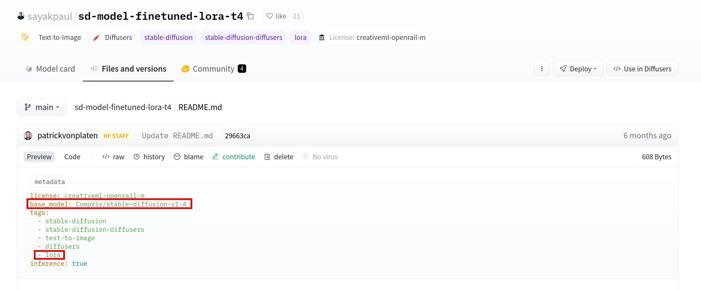 A LoRA will have a ```base_model``` attribute. This is simply the model which the LoRA was built for and should be applied to when performing inference. Because LoRAs are not the only models with such an attribute (any duplicated model will have one), a LoRA will also need a ```lora``` tag to be properly identified. ### Loading/Offloading LoRA for Diffusers 🧨 Note that there is a more seemless way to perform the same as what is presented in this section using the peft library. Please refer to the documentation for more details. The principle remains the same as below (going from/to the blue box to/from the yellow one in the diagram above)
4 functions are used in the Diffusers library to load and unload distinct LoRA weights: ```load_lora_weights``` and ```fuse_lora``` for loading and merging weights with the main layers. Note that merging weights with the main model before performing inference can decrease the inference time by 30%. ```unload_lora_weights``` and ```unfuse_lora``` for unloading. We provide an example below on how one can leverage the Diffusers library to quickly load several LoRA weights on top of a base model: ```py import torch from diffusers import ( AutoencoderKL, DiffusionPipeline, ) import time base = ""stabilityai/stable-diffusion-xl-base-1.0"" adapter1 = 'nerijs/pixel-art-xl' weightname1 = 'pixel-art-xl.safetensors' adapter2 = 'minimaxir/sdxl-wrong-lora' weightname2 = None inputs = ""elephant"" kwargs = {} if torch.cuda.is_available(): kwargs[""torch_dtype""] = torch.float16 start = time.time() # Load VAE compatible with fp16 created by madebyollin vae = AutoencoderKL.from_pretrained( ""madebyollin/sdxl-vae-fp16-fix"", torch_dtype=torch.float16, ) kwargs[""vae""] = vae kwargs[""variant""] = ""fp16"" model = DiffusionPipeline.from_pretrained( base, **kwargs ) if torch.cuda.is_available(): model.to(""cuda"") elapsed = time.time() - start print(f""Base model loaded, elapsed {elapsed:.2f} seconds"") def inference(adapter, weightname): start = time.time() model.load_lora_weights(adapter, weight_name=weightname) # Fusing lora weights with the main layers improves inference time by 30 % ! model.fuse_lora() elapsed = time.time() - start print(f""LoRA adapter loaded and fused to main model, elapsed {elapsed:.2f} seconds"") start = time.time() data = model(inputs, num_inference_steps=25).images[0] elapsed = time.time() - start print(f""Inference time, elapsed {elapsed:.2f} seconds"") start = time.time() model.unfuse_lora() model.unload_lora_weights() elapsed = time.time() - start print(f""LoRA adapter unfused/unloaded from base model, elapsed {elapsed:.2f} seconds"") inference(adapter1, weightname1) inference(adapter2, weightname2) ``` ## Loading figures All numbers below are in seconds: | GPU | T4 | A10G |
| Base model loading - not cached | 20 | 20 |
| Base model loading - cached | 5.95 | 4.09 |
| Adapter 1 loading | 3.07 | 3.46 |
| Adapter 1 unloading | 0.52 | 0.28 |
| Adapter 2 loading | 1.44 | 2.71 |
| Adapter 2 unloading | 0.19 | 0.13 |
| Inference time | 20.7 | 8.5 |
With 2 to 4 additional seconds per inference, we can serve many distinct LoRAs. However, on an A10G GPU, the inference time decreases by a lot while the adapters loading time does not change much, so the LoRA's loading/unloading is relatively more expensive. ### Serving requests To serve inference requests, we use [this open source community image](https://github.com/huggingface/api-inference-community/tree/main/docker_images/diffusers) You can find the previously described mechanism used in the [TextToImagePipeline](https://github.com/huggingface/api-inference-community/blob/main/docker_images/diffusers/app/pipelines/text_to_image.py) class. When a LoRA is requested, we'll look at the one that is loaded and change it only if required, then we perform inference as usual. This way, we are able to serve requests for the base model and many distinct adapters. Below is an example on how you can test and request this image: ``` $ git clone https://github.com/huggingface/api-inference-community.git $ cd api-inference-community/docker_images/diffusers $ docker build -t test:1.0 -f Dockerfile . $ cat > /tmp/env_file <<'EOF' MODEL_ID=stabilityai/stable-diffusion-xl-base-1.0 TASK=text-to-image HF_HUB_ENABLE_HF_TRANSFER=1 EOF $ docker run --gpus all --rm --name test1 --env-file /tmp/env_file_minimal -p 8888:80 -it test:1.0 ``` Then in another terminal perform requests to the base model and/or miscellaneous LoRA adapters to be found on the HF Hub. ``` # Request the base model $ curl 0:8888 -d '{""inputs"": ""elephant"", ""parameters"": {""num_inference_steps"": 20}}' > /tmp/base.jpg # Request one adapter $ curl -H 'lora: minimaxir/sdxl-wrong-lora' 0:8888 -d '{""inputs"": ""elephant"", ""parameters"": {""num_inference_steps"": 20}}' > /tmp/adapter1.jpg # Request another one $ curl -H 'lora: nerijs/pixel-art-xl' 0:8888 -d '{""inputs"": ""elephant"", ""parameters"": {""num_inference_steps"": 20}}' > /tmp/adapter2.jpg ``` ### What about batching ? Recently a really interesting [paper](https://arxiv.org/abs/2311.03285) came out, that described how to increase the throughput by performing batched inference on LoRA models. In short, all inference requests would be gathered in a batch, the computation related to the common base model would be done all at once, then the remaining adapter-specific products would be computed. We did not implement such a technique (close to the approach adopted in [text-generation-inference](https://github.com/huggingface/text-generation-inference/) for LLMs). Instead, we stuck to single sequential inference requests. The reason is that we observed that batching was not interesting for diffusers: throughput does not increase significantly with batch size. On the simple image generation benchmark we performed, it only increased 25% for a batch size of 8, in exchange for 6 times increased latency! Comparatively, batching is far more interesting for LLMs because you get 8 times the sequential throughput with only a 10% latency increase. This is the reason why we did not implement batching for diffusers. ## Conclusion: **Time**! Using dynamic LoRA loading, we were able to save compute resources and improve the user experience in the Hub Inference API. Despite the extra time added by the process of unloading the previously loaded adapter and loading the one we're interested in, the fact that the serving process is most often already up and running makes the inference time response on the whole much shorter. Note that for a LoRA to benefit from this inference optimization on the Hub, it must both be public, non-gated and based on a non-gated public model. Please do let us know if you apply the same method to your deployment!"
Optimum-NVIDIA - Unlock blazingly fast LLM inference in just 1 line of code,laikh-nvidia,"December 5, 2023",optimum-nvidia,"llm, nvidia, llama, inference, optimum",https://huggingface.co/blog/optimum-nvidia," # Optimum-NVIDIA on Hugging Face enables blazingly fast LLM inference in just 1 line of code Large Language Models (LLMs) have revolutionized natural language processing and are increasingly deployed to solve complex problems at scale. Achieving optimal performance with these models is notoriously challenging due to their unique and intense computational demands. Optimized performance of LLMs is incredibly valuable for end users looking for a snappy and responsive experience, as well as for scaled deployments where improved throughput translates to dollars saved. That's where the [Optimum-NVIDIA](https://github.com/huggingface/optimum-nvidia) inference library comes in. Available on Hugging Face, Optimum-NVIDIA dramatically accelerates LLM inference on the NVIDIA platform through an extremely simple API. By changing **just a single line of code**, you can unlock up to **28x faster inference and 1,200 tokens/second** on the NVIDIA platform. Optimum-NVIDIA is the first Hugging Face inference library to benefit from the new `float8` format supported on the NVIDIA Ada Lovelace and Hopper architectures. FP8, in addition to the advanced compilation capabilities of [NVIDIA TensorRT-LLM software](https://developer.nvidia.com/blog/nvidia-tensorrt-llm-supercharges-large-language-model-inference-on-nvidia-h100-gpus/) software, dramatically accelerates LLM inference. ### How to Run You can start running LLaMA with blazingly fast inference speeds in just 3 lines of code with a pipeline from Optimum-NVIDIA. If you already set up a pipeline from Hugging Face’s transformers library to run LLaMA, you just need to modify a single line of code to unlock peak performance! ```diff - from transformers.pipelines import pipeline + from optimum.nvidia.pipelines import pipeline # everything else is the same as in transformers! pipe = pipeline('text-generation', 'meta-llama/Llama-2-7b-chat-hf', use_fp8=True) pipe(""Describe a real-world application of AI in sustainable energy."") ``` You can also enable FP8 quantization with a single flag, which allows you to run a bigger model on a single GPU at faster speeds and without sacrificing accuracy. The flag shown in this example uses a predefined calibration strategy by default, though you can provide your own calibration dataset and customized tokenization to tailor the quantization to your use case. The pipeline interface is great for getting up and running quickly, but power users who want fine-grained control over setting sampling parameters can use the Model API. ```diff - from transformers import AutoModelForCausalLM + from optimum.nvidia import AutoModelForCausalLM from transformers import AutoTokenizer tokenizer = AutoTokenizer.from_pretrained(""meta-llama/Llama-2-13b-chat-hf"", padding_side=""left"") model = AutoModelForCausalLM.from_pretrained( ""meta-llama/Llama-2-13b-chat-hf"", + use_fp8=True, ) model_inputs = tokenizer( [""How is autonomous vehicle technology transforming the future of transportation and urban planning?""], return_tensors=""pt"" ).to(""cuda"") generated_ids, generated_length = model.generate( **model_inputs, top_k=40, top_p=0.7, repetition_penalty=10, ) tokenizer.batch_decode(generated_ids[0], skip_special_tokens=True) ``` For more details, check out our [documentation](https://github.com/huggingface/optimum-nvidia) ### Performance Evaluation When evaluating the performance of an LLM, we consider two metrics: First Token Latency and Throughput. First Token Latency (also known as Time to First Token or prefill latency) measures how long you wait from the time you enter your prompt to the time you begin receiving your output, so this metric can tell you how responsive the model will feel. Optimum-NVIDIA delivers up to 3.3x faster First Token Latency compared to stock transformers:
![]() Figure 1. Time it takes to generate the first token (ms)
Figure 1. Time it takes to generate the first token (ms)
Throughput, on the other hand, measures how fast the model can generate tokens and is particularly relevant when you want to batch generations together. While there are a few ways to calculate throughput, we adopted a standard method to divide the end-to-end latency by the total sequence length, including both input and output tokens summed over all batches. Optimum-NVIDIA delivers up to 28x better throughput compared to stock transformers:
![]() Figure 2. Throughput (token / second)
Figure 2. Throughput (token / second)
Initial evaluations of the [recently announced NVIDIA H200 Tensor Core GPU](https://www.nvidia.com/en-us/data-center/h200/) show up to an additional 2x boost in throughput for LLaMA models compared to an NVIDIA H100 Tensor Core GPU. As H200 GPUs become more readily available, we will share performance data for Optimum-NVIDIA running on them. ### Next steps Optimum-NVIDIA currently provides peak performance for the LLaMAForCausalLM architecture + task, so any [LLaMA-based model](https://huggingface.co/models?other=llama,llama2), including fine-tuned versions, should work with Optimum-NVIDIA out of the box today. We are actively expanding support to include other text generation model architectures and tasks, all from within Hugging Face. We continue to push the boundaries of performance and plan to incorporate cutting-edge optimization techniques like In-Flight Batching to improve throughput when streaming prompts and INT4 quantization to run even bigger models on a single GPU. Give it a try: we are releasing the [Optimum-NVIDIA repository](https://github.com/huggingface/optimum-nvidia) with instructions on how to get started. Please share your feedback with us! 🤗"
SetFitABSA: Few-Shot Aspect Based Sentiment Analysis using SetFit,ronenlap,"December 6, 2023",setfit-absa,"research, nlp",https://huggingface.co/blog/setfit-absa," # SetFitABSA: Few-Shot Aspect Based Sentiment Analysis using SetFit ![]()
SetFitABSA is an efficient technique to detect the sentiment towards specific aspects within the text.
Aspect-Based Sentiment Analysis (ABSA) is the task of detecting the sentiment towards specific aspects within the text. For example, in the sentence, ""This phone has a great screen, but its battery is too small"", the _aspect_ terms are ""screen"" and ""battery"" and the sentiment polarities towards them are Positive and Negative, respectively. ABSA is widely used by organizations for extracting valuable insights by analyzing customer feedback towards aspects of products or services in various domains. However, labeling training data for ABSA is a tedious task because of the fine-grained nature (token level) of manually identifying aspects within the training samples. Intel Labs and Hugging Face are excited to introduce SetFitABSA, a framework for few-shot training of domain-specific ABSA models; SetFitABSA is competitive and even outperforms generative models such as Llama2 and T5 in few-shot scenarios. Compared to LLM based methods, SetFitABSA has two unique advantages: 🗣 No prompts needed: few-shot in-context learning with LLMs requires handcrafted prompts which make the results brittle, sensitive to phrasing and dependent on user expertise. SetFitABSA dispenses with prompts altogether by generating rich embeddings directly from a small number of labeled text examples.
🏎 Fast to train: SetFitABSA requires only a handful of labeled training samples; in addition, it uses a simple training data format, eliminating the need for specialized tagging tools. This makes the data labeling process fast and easy.
In this blog post, we'll explain how SetFitABSA works and how to train your very own models using the [SetFit library](https://github.com/huggingface/setfit). Let's dive in! ## How does it work? ![]()
SetFitABSA's three-stage training process
SetFitABSA is comprised of three steps. The first step extracts aspect candidates from the text, the second one yields the aspects by classifying the aspect candidates as aspects or non-aspects, and the final step associates a sentiment polarity to each extracted aspect. Steps two and three are based on SetFit models. ### Training **1. Aspect candidate extraction** In this work we assume that aspects, which are usually features of products and services, are mostly nouns or noun compounds (strings of consecutive nouns). We use [spaCy](https://spacy.io/) to tokenize and extract nouns/noun compounds from the sentences in the (few-shot) training set. Since not all extracted nouns/noun compounds are aspects, we refer to them as aspect candidates. **2. Aspect/Non-aspect classification** Now that we have aspect candidates, we need to train a model to be able to distinguish between nouns that are aspects and nouns that are non-aspects. For this purpose, we need training samples with aspect/no-aspect labels. This is done by considering aspects in the training set as `True` aspects, while other non-overlapping candidate aspects are considered non-aspects and therefore labeled as `False`: * **Training sentence:** ""Waiters aren't friendly but the cream pasta is out of this world."" * **Tokenized:** [Waiters, are, n't, friendly, but, the, cream, pasta, is, out, of, this, world, .] * **Extracted aspect candidates:** [Waiters, are, n't, friendly, but, the, cream, pasta, is, out, of, this, world, .] * **Gold labels from training set, in [BIO format](https://en.wikipedia.org/wiki/Inside–outside–beginning_(tagging)):** [B-ASP, O, O, O, O, O, B-ASP, I-ASP, O, O, O, O, O, .] * **Generated aspect/non-aspect Labels:** [Waiters, are, n't, friendly, but, the, cream, pasta, is, out, of, this, world, .] Now that we have all the aspect candidates labeled, how do we use it to train the candidate aspect classification model? In other words, how do we use SetFit, a sentence classification framework, to classify individual tokens? Well, this is the trick: each aspect candidate is concatenated with the entire training sentence to create a training instance using the following template: ``` aspect_candidate:training_sentence ``` Applying the template to the example above will generate 3 training instances – two with `True` labels representing aspect training instances, and one with `False` label representing non-aspect training instance: | Text | Label | |:------------------------------------------------------------------------------|:------| | Waiters:Waiters aren't friendly but the cream pasta is out of this world. | 1 | | cream pasta:Waiters aren't friendly but the cream pasta is out of this world. | 1 | | world:Waiters aren't friendly but the cream pasta is out of this world. | 0 | | ... | ... | After generating the training instances, we are ready to use the power of SetFit to train a few-shot domain-specific binary classifier to extract aspects from an input text review. This will be our first fine-tuned SetFit model. **3. Sentiment polarity classification** Once the system extracts the aspects from the text, it needs to associate a sentiment polarity (e.g., positive, negative or neutral) to each aspect. For this purpose, we use a 2nd SetFit model and train it in a similar fashion to the aspect extraction model as illustrated in the following example: * **Training sentence:** ""Waiters aren't friendly but the cream pasta is out of this world."" * **Tokenized:** [Waiters, are, n't, friendly, but, the, cream, pasta, is, out, of, this, world, .] * **Gold labels from training set:** [NEG, O, O, O, O, O, POS, POS, O, O, O, O, O, .] | Text | Label | |:------------------------------------------------------------------------------|:------| | Waiters:Waiters aren't friendly but the cream pasta is out of this world. | NEG | | cream pasta:Waiters aren't friendly but the cream pasta is out of this world. | POS | | ... | ... | Note that as opposed to the aspect extraction model, we don't include non-aspects in this training set because the goal is to classify the sentiment polarity towards real aspects. ## Running inference At inference time, the test sentence passes through the spaCy aspect candidate extraction phase, resulting in test instances using the template `aspect_candidate:test_sentence`. Next, non-aspects are filtered by the aspect/non-aspect classifier. Finally, the extracted aspects are fed to the sentiment polarity classifier that predicts the sentiment polarity per aspect. In practice, this means the model can receive normal text as input, and output aspects and their sentiments: **Model Input:** ``` ""their dinner specials are fantastic."" ``` **Model Output:** ``` [{'span': 'dinner specials', 'polarity': 'positive'}] ``` ## Benchmarking SetFitABSA was benchmarked against the recent state-of-the-art work by [AWS AI Labs](https://arxiv.org/pdf/2210.06629.pdf) and [Salesforce AI Research](https://arxiv.org/pdf/2204.05356.pdf) that finetune T5 and GPT2 using prompts. To get a more complete picture, we also compare our model to the Llama-2-chat model using in-context learning. We use the popular Laptop14 and Restaurant14 ABSA [datasets](https://huggingface.co/datasets/alexcadillon/SemEval2014Task4) from the Semantic Evaluation Challenge 2014 ([SemEval14](https://aclanthology.org/S14-2004.pdf)). SetFitABSA is evaluated both on the intermediate task of aspect term extraction (SB1) and on the full ABSA task of aspect extraction along with their sentiment polarity predictions (SB1+SB2). ### Model size comparison | Model | Size (params) | |:------------------:|:-------------:| | Llama-2-chat | 7B | | T5-base | 220M | | GPT2-base | 124M | | GPT2-medium | 355M | | **SetFit (MPNet)** | 2x 110M | Note that for the SB1 task, SetFitABSA is 110M parameters, for SB2 it is 110M parameters, and for SB1+SB2 SetFitABSA consists of 220M parameters. ### Performance comparison We see a clear advantage of SetFitABSA when the number of training instances is low, despite being 2x smaller than T5 and x3 smaller than GPT2-medium. Even when compared to Llama 2, which is x64 larger, the performance is on par or better. **SetFitABSA vs GPT2** ![]()
**SetFitABSA vs T5** ![]()
Note that for fair comparison, we conducted comparisons with SetFitABSA against exactly the dataset splits used by the various baselines (GPT2, T5, etc.). **SetFitABSA vs Llama2** ![]()
We notice that increasing the number of in-context training samples for Llama2 did not result in improved performance. This phenomenon [has been shown for ChatGPT before](https://www.analyticsvidhya.com/blog/2023/09/power-of-llms-zero-shot-and-few-shot-prompting/), and we think it should be further investigated. ## Training your own model SetFitABSA is part of the SetFit framework. To train an ABSA model, start by installing `setfit` with the `absa` option enabled: ```shell python -m pip install -U ""setfit[absa]"" ``` Additionally, we must install the `en_core_web_lg` spaCy model: ```shell python -m spacy download en_core_web_lg ``` We continue by preparing the training set. The format of the training set is a `Dataset` with the columns `text`, `span`, `label`, `ordinal`: * **text**: The full sentence or text containing the aspects. * **span**: An aspect from the full sentence. Can be multiple words. For example: ""food"". * **label**: The (polarity) label corresponding to the aspect span. For example: ""positive"". The label names can be chosen arbitrarily when tagging the collected training data. * **ordinal**: If the aspect span occurs multiple times in the text, then this ordinal represents the index of those occurrences. Often this is just 0, as each aspect usually appears only once in the input text. For example, the training text ""Restaurant with wonderful food but worst service I ever seen"" contains two aspects, so will add two lines to the training set table: | Text | Span | Label | Ordinal | |:-------------------------------------------------------------|:--------|:---------|:--------| | Restaurant with wonderful food but worst service I ever seen | food | positive | 0 | | Restaurant with wonderful food but worst service I ever seen | service | negative | 0 | | ... | ... | ... | ... | Once we have the training dataset ready we can create an ABSA trainer and execute the training. SetFit models are fairly efficient to train, but as SetFitABSA involves two models trained sequentially, it is recommended to use a GPU for training to keep the training time low. For example, the following training script trains a full SetFitABSA model in about 10 minutes with the free Google Colab T4 GPU. ```python from datasets import load_dataset from setfit import AbsaTrainer, AbsaModel # Create a training dataset as above # For convenience we will use an already prepared dataset here train_dataset = load_dataset(""tomaarsen/setfit-absa-semeval-restaurants"", split=""train[:128]"") # Create a model with a chosen sentence transformer from the Hub model = AbsaModel.from_pretrained(""sentence-transformers/paraphrase-mpnet-base-v2"") # Create a trainer: trainer = AbsaTrainer(model, train_dataset=train_dataset) # Execute training: trainer.train() ``` That's it! We have trained a domain-specific ABSA model. We can save our trained model to disk or upload it to the Hugging Face hub. Bear in mind that the model contains two submodels, so each is given its own path: ```python model.save_pretrained( ""models/setfit-absa-model-aspect"", ""models/setfit-absa-model-polarity"" ) # or model.push_to_hub( ""tomaarsen/setfit-absa-paraphrase-mpnet-base-v2-restaurants-aspect"", ""tomaarsen/setfit-absa-paraphrase-mpnet-base-v2-restaurants-polarity"" ) ``` Now we can use our trained model for inference. We start by loading the model: ```python from setfit import AbsaModel model = AbsaModel.from_pretrained( ""tomaarsen/setfit-absa-paraphrase-mpnet-base-v2-restaurants-aspect"", ""tomaarsen/setfit-absa-paraphrase-mpnet-base-v2-restaurants-polarity"" ) ``` Then, we use the predict API to run inference. The input is a list of strings, each representing a textual review: ```python preds = model.predict([ ""Best pizza outside of Italy and really tasty."", ""The food variations are great and the prices are absolutely fair."", ""Unfortunately, you have to expect some waiting time and get a note with a waiting number if it should be very full."" ]) print(preds) # [ # [{'span': 'pizza', 'polarity': 'positive'}], # [{'span': 'food variations', 'polarity': 'positive'}, {'span': 'prices', 'polarity': 'positive'}], # [{'span': 'waiting time', 'polarity': 'neutral'}, {'span': 'waiting number', 'polarity': 'neutral'}] # ] ``` For more details on training options, saving and loading models, and inference see the SetFit [docs](https://huggingface.co/docs/setfit/how_to/absa). ## References * Maria Pontiki, Dimitris Galanis, John Pavlopoulos, Harris Papageorgiou, Ion Androutsopoulos, and Suresh Manandhar. 2014. SemEval-2014 task 4: Aspect based sentiment analysis. In Proceedings of the 8th International Workshop on Semantic Evaluation (SemEval 2014), pages 27–35. * Siddharth Varia, Shuai Wang, Kishaloy Halder, Robert Vacareanu, Miguel Ballesteros, Yassine Benajiba, Neha Anna John, Rishita Anubhai, Smaranda Muresan, Dan Roth, 2023 ""Instruction Tuning for Few-Shot Aspect-Based Sentiment Analysis"". https://arxiv.org/abs/2210.06629 * Ehsan Hosseini-Asl, Wenhao Liu, Caiming Xiong, 2022. ""A Generative Language Model for Few-shot Aspect-Based Sentiment Analysis"". https://arxiv.org/abs/2204.05356 * Lewis Tunstall, Nils Reimers, Unso Eun Seo Jo, Luke Bates, Daniel Korat, Moshe Wasserblat, Oren Pereg, 2022. ""Efficient Few-Shot Learning Without Prompts"". https://arxiv.org/abs/2209.11055"