text,source
"---
draft: false
title: Food Discovery
short_description: Qdrant Food Discovery Demo recommends more similar meals based on how they look
description: This demo uses data from Delivery Service. Users may like or dislike the photo of a dish, and the app will recommend more similar meals based on how they look. It's also possible to choose to view results from the restaurants within the delivery radius.
preview_image: /demo/food-discovery-demo.png
link: https://food-discovery.qdrant.tech/
weight: 2
sitemapExclude: True
---
",demo/demo-2.md
"---
draft: false
title: E-commerce products categorization
short_description: E-commerce products categorization demo from Qdrant vector database
description: This demo shows how you can use vector database in e-commerce. Enter the name of the product and the application will understand which category it belongs to, based on the multi-language model. The dots represent clusters of products.
preview_image: /demo/products_categorization_demo.jpg
link: https://qdrant.to/extreme-classification-demo
weight: 3
sitemapExclude: True
---
",demo/demo-3.md
"---
draft: false
title: Startup Search
short_description: Qdrant Startup Search. This demo uses short descriptions of startups to perform a semantic search
description: This demo uses short descriptions of startups to perform a semantic search. Each startup description converted into a vector using a pre-trained SentenceTransformer model and uploaded to the Qdrant vector search engine. Demo service processes text input with the same model and uses its output to query Qdrant for similar vectors. You can turn neural search on and off to compare the result with regular full-text search.
preview_image: /demo/startup_search_demo.jpg
link: https://qdrant.to/semantic-search-demo
weight: 1
sitemapExclude: True
---
",demo/demo-1.md
"---
page_title: Vector Search Demos and Examples
description: Interactive examples and demos of vector search based applications developed with Qdrant vector search engine.
title: Vector Search Demos
section_title: Interactive Live Examples
---",demo/_index.md
"---
title: Examples
weight: 25
# If the index.md file is empty, the link to the section will be hidden from the sidebar
is_empty: false
---
# Sample Use Cases
Our Notebooks offer complex instructions that are supported with a throrough explanation. Follow along by trying out the code and get the most out of each example.
| Example | Description | Stack |
|---------------------------------------------------------------------------------------------------------------------------------------------------------------------------------------------------------------------------------------|-------------------------------------------------------------------------------------------------|----------------------------|
| [Intro to Semantic Search and Recommendations Systems](https://githubtocolab.com/qdrant/examples/blob/master/qdrant_101_getting_started/getting_started.ipynb) | Learn how to get started building semantic search and recommendation systems. | Qdrant |
| [Search and Recommend Newspaper Articles](https://githubtocolab.com/qdrant/examples/blob/master/qdrant_101_text_data/qdrant_and_text_data.ipynb) | Work with text data to develop a semantic search and a recommendation engine for news articles. | Qdrant |
| [Recommendation System for Songs](https://githubtocolab.com/qdrant/examples/blob/master/qdrant_101_audio_data/03_qdrant_101_audio.ipynb) | Use Qdrant to develop a music recommendation engine based on audio embeddings. | Qdrant |
| [Image Comparison System for Skin Conditions](https://colab.research.google.com/github/qdrant/examples/blob/master/qdrant_101_image_data/04_qdrant_101_cv.ipynb) | Use Qdrant to compare challenging images with labels representing different skin diseases. | Qdrant |
| [Question and Answer System with LlamaIndex](https://githubtocolab.com/qdrant/examples/blob/master/llama_index_recency/Qdrant%20and%20LlamaIndex%20%E2%80%94%20A%20new%20way%20to%20keep%20your%20Q%26A%20systems%20up-to-date.ipynb) | Combine Qdrant and LlamaIndex to create a self-updating Q&A system. | Qdrant, LlamaIndex, Cohere |
| [Extractive QA System](https://githubtocolab.com/qdrant/examples/blob/master/extractive_qa/extractive-question-answering.ipynb) | Extract answers directly from context to generate highly relevant answers. | Qdrant |
| [Ecommerce Reverse Image Search](https://githubtocolab.com/qdrant/examples/blob/master/ecommerce_reverse_image_search/ecommerce-reverse-image-search.ipynb) | Accept images as search queries to receive semantically appropriate answers. | Qdrant |
| [Basic RAG](https://githubtocolab.com/qdrant/examples/blob/master/rag-openai-qdrant/rag-openai-qdrant.ipynb) | Basic RAG pipeline with Qdrant and OpenAI SDKs | OpenAI, Qdrant, FastEmbed |
",documentation/examples.md
"---
title: Release notes
weight: 42
type: external-link
external_url: https://github.com/qdrant/qdrant/releases
sitemapExclude: True
---
",documentation/release-notes.md
"---
title: Benchmarks
weight: 33
draft: true
---
",documentation/benchmarks.md
"---
title: Community links
weight: 42
---
# Community Contributions
Though we do not officially maintain this content, we still feel that is is valuable and thank our dedicated contributors.
| Link | Description | Stack |
|------|------------------------------|--------|
| [Pinecone to Qdrant Migration](https://github.com/NirantK/qdrant_tools) | Complete python toolset that supports migration between two products. | Qdrant, Pinecone |
| [LlamaIndex Support for Qdrant](https://gpt-index.readthedocs.io/en/latest/examples/vector_stores/QdrantIndexDemo.html) | Documentation on common integrations with LlamaIndex. | Qdrant, LlamaIndex |
| [Geo.Rocks Semantic Search Tutorial](https://geo.rocks/post/qdrant-transformers-js-semantic-search/) | Create a fully working semantic search stack with a built in search API and a minimal stack. | Qdrant, HuggingFace, SentenceTransformers, transformers.js |
",documentation/community-links.md
"---
title: Quickstart
weight: 11
aliases:
- quick_start
---
# Quickstart
In this short example, you will use the Python Client to create a Collection, load data into it and run a basic search query.
## Download and run
First, download the latest Qdrant image from Dockerhub:
```bash
docker pull qdrant/qdrant
```
Then, run the service:
```bash
docker run -p 6333:6333 -p 6334:6334 \
-v $(pwd)/qdrant_storage:/qdrant/storage:z \
qdrant/qdrant
```
Under the default configuration all data will be stored in the `./qdrant_storage` directory. This will also be the only directory that both the Container and the host machine can both see.
Qdrant is now accessible:
- REST API: [localhost:6333](http://localhost:6333)
- Web UI: [localhost:6333/dashboard](http://localhost:6333/dashboard)
- GRPC API: [localhost:6334](http://localhost:6334)
## Initialize the client
```python
from qdrant_client import QdrantClient
client = QdrantClient(""localhost"", port=6333)
```
```typescript
import { QdrantClient } from ""@qdrant/js-client-rest"";
const client = new QdrantClient({ host: ""localhost"", port: 6333 });
```
```rust
use qdrant_client::client::QdrantClient;
// The Rust client uses Qdrant's GRPC interface
let client = QdrantClient::from_url(""http://localhost:6334"").build()?;
```
```java
import io.qdrant.client.QdrantClient;
import io.qdrant.client.QdrantGrpcClient;
// The Java client uses Qdrant's GRPC interface
QdrantClient client = new QdrantClient(
QdrantGrpcClient.newBuilder(""localhost"", 6334, false).build());
```
```csharp
using Qdrant.Client;
// The C# client uses Qdrant's GRPC interface
var client = new QdrantClient(""localhost"", 6334);
```
## Create a collection
You will be storing all of your vector data in a Qdrant collection. Let's call it `test_collection`. This collection will be using a dot product distance metric to compare vectors.
```python
from qdrant_client.http.models import Distance, VectorParams
client.create_collection(
collection_name=""test_collection"",
vectors_config=VectorParams(size=4, distance=Distance.DOT),
)
```
```typescript
await client.createCollection(""test_collection"", {
vectors: { size: 4, distance: ""Dot"" },
});
```
```rust
use qdrant_client::qdrant::{vectors_config::Config, VectorParams, VectorsConfig};
client
.create_collection(&CreateCollection {
collection_name: ""test_collection"".to_string(),
vectors_config: Some(VectorsConfig {
config: Some(Config::Params(VectorParams {
size: 4,
distance: Distance::Dot.into(),
..Default::default()
})),
}),
..Default::default()
})
.await?;
```
```java
import io.qdrant.client.grpc.Collections.Distance;
import io.qdrant.client.grpc.Collections.VectorParams;
client.createCollectionAsync(""test_collection"",
VectorParams.newBuilder().setDistance(Distance.Dot).setSize(4).build()).get();
```
```csharp
using Qdrant.Client.Grpc;
await client.CreateCollectionAsync(
collectionName: ""test_collection"",
vectorsConfig: new VectorParams { Size = 4, Distance = Distance.Dot }
);
```
## Add vectors
Let's now add a few vectors with a payload. Payloads are other data you want to associate with the vector:
```python
from qdrant_client.http.models import PointStruct
operation_info = client.upsert(
collection_name=""test_collection"",
wait=True,
points=[
PointStruct(id=1, vector=[0.05, 0.61, 0.76, 0.74], payload={""city"": ""Berlin""}),
PointStruct(id=2, vector=[0.19, 0.81, 0.75, 0.11], payload={""city"": ""London""}),
PointStruct(id=3, vector=[0.36, 0.55, 0.47, 0.94], payload={""city"": ""Moscow""}),
PointStruct(id=4, vector=[0.18, 0.01, 0.85, 0.80], payload={""city"": ""New York""}),
PointStruct(id=5, vector=[0.24, 0.18, 0.22, 0.44], payload={""city"": ""Beijing""}),
PointStruct(id=6, vector=[0.35, 0.08, 0.11, 0.44], payload={""city"": ""Mumbai""}),
],
)
print(operation_info)
```
```typescript
const operationInfo = await client.upsert(""test_collection"", {
wait: true,
points: [
{ id: 1, vector: [0.05, 0.61, 0.76, 0.74], payload: { city: ""Berlin"" } },
{ id: 2, vector: [0.19, 0.81, 0.75, 0.11], payload: { city: ""London"" } },
{ id: 3, vector: [0.36, 0.55, 0.47, 0.94], payload: { city: ""Moscow"" } },
{ id: 4, vector: [0.18, 0.01, 0.85, 0.80], payload: { city: ""New York"" } },
{ id: 5, vector: [0.24, 0.18, 0.22, 0.44], payload: { city: ""Beijing"" } },
{ id: 6, vector: [0.35, 0.08, 0.11, 0.44], payload: { city: ""Mumbai"" } },
],
});
console.debug(operationInfo);
```
```rust
use qdrant_client::qdrant::PointStruct;
use serde_json::json;
let points = vec![
PointStruct::new(
1,
vec![0.05, 0.61, 0.76, 0.74],
json!(
{""city"": ""Berlin""}
)
.try_into()
.unwrap(),
),
PointStruct::new(
2,
vec![0.19, 0.81, 0.75, 0.11],
json!(
{""city"": ""London""}
)
.try_into()
.unwrap(),
),
// ..truncated
];
let operation_info = client
.upsert_points_blocking(""test_collection"".to_string(), None, points, None)
.await?;
dbg!(operation_info);
```
```java
import java.util.List;
import java.util.Map;
import static io.qdrant.client.PointIdFactory.id;
import static io.qdrant.client.ValueFactory.value;
import static io.qdrant.client.VectorsFactory.vectors;
import io.qdrant.client.grpc.Points.PointStruct;
import io.qdrant.client.grpc.Points.UpdateResult;
UpdateResult operationInfo =
client
.upsertAsync(
""test_collection"",
List.of(
PointStruct.newBuilder()
.setId(id(1))
.setVectors(vectors(0.05f, 0.61f, 0.76f, 0.74f))
.putAllPayload(Map.of(""city"", value(""Berlin"")))
.build(),
PointStruct.newBuilder()
.setId(id(2))
.setVectors(vectors(0.19f, 0.81f, 0.75f, 0.11f))
.putAllPayload(Map.of(""city"", value(""London"")))
.build(),
PointStruct.newBuilder()
.setId(id(3))
.setVectors(vectors(0.36f, 0.55f, 0.47f, 0.94f))
.putAllPayload(Map.of(""city"", value(""Moscow"")))
.build()))
// Truncated
.get();
System.out.println(operationInfo);
```
```csharp
using Qdrant.Client.Grpc;
var operationInfo = await client.UpsertAsync(
collectionName: ""test_collection"",
points: new List
{
new()
{
Id = 1,
Vectors = new float[] { 0.05f, 0.61f, 0.76f, 0.74f },
Payload = { [""city""] = ""Berlin"" }
},
new()
{
Id = 2,
Vectors = new float[] { 0.19f, 0.81f, 0.75f, 0.11f },
Payload = { [""city""] = ""London"" }
},
new()
{
Id = 3,
Vectors = new float[] { 0.36f, 0.55f, 0.47f, 0.94f },
Payload = { [""city""] = ""Moscow"" }
},
// Truncated
}
);
Console.WriteLine(operationInfo);
```
**Response:**
```python
operation_id=0 status=
```
```typescript
{ operation_id: 0, status: 'completed' }
```
```rust
PointsOperationResponse {
result: Some(UpdateResult {
operation_id: 0,
status: Completed,
}),
time: 0.006347708,
}
```
```java
operation_id: 0
status: Completed
```
```csharp
{ ""operationId"": ""0"", ""status"": ""Completed"" }
```
## Run a query
Let's ask a basic question - Which of our stored vectors are most similar to the query vector `[0.2, 0.1, 0.9, 0.7]`?
```python
search_result = client.search(
collection_name=""test_collection"", query_vector=[0.2, 0.1, 0.9, 0.7], limit=3
)
print(search_result)
```
```typescript
let searchResult = await client.search(""test_collection"", {
vector: [0.2, 0.1, 0.9, 0.7],
limit: 3,
});
console.debug(searchResult);
```
```rust
use qdrant_client::qdrant::SearchPoints;
let search_result = client
.search_points(&SearchPoints {
collection_name: ""test_collection"".to_string(),
vector: vec![0.2, 0.1, 0.9, 0.7],
limit: 3,
with_payload: Some(true.into()),
..Default::default()
})
.await?;
dbg!(search_result);
```
```java
import java.util.List;
import io.qdrant.client.grpc.Points.ScoredPoint;
import io.qdrant.client.grpc.Points.SearchPoints;
import static io.qdrant.client.WithPayloadSelectorFactory.enable;
List searchResult =
client
.searchAsync(
SearchPoints.newBuilder()
.setCollectionName(""test_collection"")
.setLimit(3)
.addAllVector(List.of(0.2f, 0.1f, 0.9f, 0.7f))
.setWithPayload(enable(true))
.build())
.get();
System.out.println(searchResult);
```
```csharp
var searchResult = await client.SearchAsync(
collectionName: ""test_collection"",
vector: new float[] { 0.2f, 0.1f, 0.9f, 0.7f },
limit: 3,
payloadSelector: true
);
Console.WriteLine(searchResult);
```
**Response:**
```python
ScoredPoint(id=4, version=0, score=1.362, payload={""city"": ""New York""}, vector=None),
ScoredPoint(id=1, version=0, score=1.273, payload={""city"": ""Berlin""}, vector=None),
ScoredPoint(id=3, version=0, score=1.208, payload={""city"": ""Moscow""}, vector=None)
```
```typescript
[
{
id: 4,
version: 0,
score: 1.362,
payload: null,
vector: null,
},
{
id: 1,
version: 0,
score: 1.273,
payload: null,
vector: null,
},
{
id: 3,
version: 0,
score: 1.208,
payload: null,
vector: null,
},
];
```
```rust
SearchResponse {
result: [
ScoredPoint {
id: Some(PointId {
point_id_options: Some(Num(4)),
}),
payload: {},
score: 1.362,
version: 0,
vectors: None,
},
ScoredPoint {
id: Some(PointId {
point_id_options: Some(Num(1)),
}),
payload: {},
score: 1.273,
version: 0,
vectors: None,
},
ScoredPoint {
id: Some(PointId {
point_id_options: Some(Num(3)),
}),
payload: {},
score: 1.208,
version: 0,
vectors: None,
},
],
time: 0.003635125,
}
```
```java
[id {
num: 4
}
payload {
key: ""city""
value {
string_value: ""New York""
}
}
score: 1.362
version: 1
, id {
num: 1
}
payload {
key: ""city""
value {
string_value: ""Berlin""
}
}
score: 1.273
version: 1
, id {
num: 3
}
payload {
key: ""city""
value {
string_value: ""Moscow""
}
}
score: 1.208
version: 1
]
```
```csharp
[
{
""id"": {
""num"": ""4""
},
""payload"": {
""city"": {
""stringValue"": ""New York""
}
},
""score"": 1.362,
""version"": ""7""
},
{
""id"": {
""num"": ""1""
},
""payload"": {
""city"": {
""stringValue"": ""Berlin""
}
},
""score"": 1.273,
""version"": ""7""
},
{
""id"": {
""num"": ""3""
},
""payload"": {
""city"": {
""stringValue"": ""Moscow""
}
},
""score"": 1.208,
""version"": ""7""
}
]
```
The results are returned in decreasing similarity order. Note that payload and vector data is missing in these results by default.
See [payload and vector in the result](../concepts/search#payload-and-vector-in-the-result) on how to enable it.
## Add a filter
We can narrow down the results further by filtering by payload. Let's find the closest results that include ""London"".
```python
from qdrant_client.http.models import Filter, FieldCondition, MatchValue
search_result = client.search(
collection_name=""test_collection"",
query_vector=[0.2, 0.1, 0.9, 0.7],
query_filter=Filter(
must=[FieldCondition(key=""city"", match=MatchValue(value=""London""))]
),
with_payload=True,
limit=3,
)
print(search_result)
```
```typescript
searchResult = await client.search(""test_collection"", {
vector: [0.2, 0.1, 0.9, 0.7],
filter: {
must: [{ key: ""city"", match: { value: ""London"" } }],
},
with_payload: true,
limit: 3,
});
console.debug(searchResult);
```
```rust
use qdrant_client::qdrant::{Condition, Filter, SearchPoints};
let search_result = client
.search_points(&SearchPoints {
collection_name: ""test_collection"".to_string(),
vector: vec![0.2, 0.1, 0.9, 0.7],
filter: Some(Filter::all([Condition::matches(
""city"",
""London"".to_string(),
)])),
limit: 2,
..Default::default()
})
.await?;
dbg!(search_result);
```
```java
import static io.qdrant.client.ConditionFactory.matchKeyword;
List searchResult =
client
.searchAsync(
SearchPoints.newBuilder()
.setCollectionName(""test_collection"")
.setLimit(3)
.setFilter(Filter.newBuilder().addMust(matchKeyword(""city"", ""London"")))
.addAllVector(List.of(0.2f, 0.1f, 0.9f, 0.7f))
.setWithPayload(enable(true))
.build())
.get();
System.out.println(searchResult);
```
```csharp
using static Qdrant.Client.Grpc.Conditions;
var searchResult = await client.SearchAsync(
collectionName: ""test_collection"",
vector: new float[] { 0.2f, 0.1f, 0.9f, 0.7f },
filter: MatchKeyword(""city"", ""London""),
limit: 3,
payloadSelector: true
);
Console.WriteLine(searchResult);
```
**Response:**
```python
ScoredPoint(id=2, version=0, score=0.871, payload={""city"": ""London""}, vector=None)
```
```typescript
[
{
id: 2,
version: 0,
score: 0.871,
payload: { city: ""London"" },
vector: null,
},
];
```
```rust
SearchResponse {
result: [
ScoredPoint {
id: Some(
PointId {
point_id_options: Some(
Num(
2,
),
),
},
),
payload: {
""city"": Value {
kind: Some(
StringValue(
""London"",
),
),
},
},
score: 0.871,
version: 0,
vectors: None,
},
],
time: 0.004001083,
}
```
```java
[id {
num: 2
}
payload {
key: ""city""
value {
string_value: ""London""
}
}
score: 0.871
version: 1
]
```
```csharp
[
{
""id"": {
""num"": ""2""
},
""payload"": {
""city"": {
""stringValue"": ""London""
}
},
""score"": 0.871,
""version"": ""7""
}
]
```
You have just conducted vector search. You loaded vectors into a database and queried the database with a vector of your own. Qdrant found the closest results and presented you with a similarity score.
## Next steps
Now you know how Qdrant works. Getting started with [Qdrant Cloud](../cloud/quickstart-cloud/) is just as easy. [Create an account](https://qdrant.to/cloud) and use our SaaS completely free. We will take care of infrastructure maintenance and software updates.
To move onto some more complex examples of vector search, read our [Tutorials](../tutorials/) and create your own app with the help of our [Examples](../examples/).
**Note:** There is another way of running Qdrant locally. If you are a Python developer, we recommend that you try Local Mode in [Qdrant Client](https://github.com/qdrant/qdrant-client), as it only takes a few moments to get setup.
",documentation/quick-start.md
"---
#Delimiter files are used to separate the list of documentation pages into sections.
title: ""Getting Started""
type: delimiter
weight: 8 # Change this weight to change order of sections
sitemapExclude: True
---",documentation/0-dl.md
"---
#Delimiter files are used to separate the list of documentation pages into sections.
title: ""Integrations""
type: delimiter
weight: 30 # Change this weight to change order of sections
sitemapExclude: True
---",documentation/2-dl.md
"---
title: Roadmap
weight: 32
draft: true
---
# Qdrant 2023 Roadmap
Goals of the release:
* **Maintain easy upgrades** - we plan to keep backward compatibility for at least one major version back.
* That means that you can upgrade Qdrant without any downtime and without any changes in your client code within one major version.
* Storage should be compatible between any two consequent versions, so you can upgrade Qdrant with automatic data migration between consecutive versions.
* **Make billion-scale serving cheap** - qdrant already can serve billions of vectors, but we want to make it even more affordable.
* **Easy scaling** - our plan is to make it easy to dynamically scale Qdrant, so you could go from 1 to 1B vectors seamlessly.
* **Various similarity search scenarios** - we want to support more similarity search scenarios, e.g. sparse search, grouping requests, diverse search, etc.
## Milestones
* :atom_symbol: Quantization support
* [ ] Scalar quantization f32 -> u8 (4x compression)
* [ ] Advanced quantization (8x and 16x compression)
* [ ] Support for binary vectors
---
* :arrow_double_up: Scalability
* [ ] Automatic replication factor adjustment
* [ ] Automatic shard distribution on cluster scaling
* [ ] Repartitioning support
---
* :eyes: Search scenarios
* [ ] Diversity search - search for vectors that are different from each other
* [ ] Sparse vectors search - search for vectors with a small number of non-zero values
* [ ] Grouping requests - search within payload-defined groups
* [ ] Different scenarios for recommendation API
---
* Additionally
* [ ] Extend full-text filtering support
* [ ] Support for phrase queries
* [ ] Support for logical operators
* [ ] Simplify update of collection parameters
",documentation/roadmap.md
"---
title: Interfaces
weight: 14
---
# Interfaces
Qdrant supports these ""official"" clients.
> **Note:** If you are using a language that is not listed here, you can use the REST API directly or generate a client for your language
using [OpenAPI](https://github.com/qdrant/qdrant/blob/master/docs/redoc/master/openapi.json)
or [protobuf](https://github.com/qdrant/qdrant/tree/master/lib/api/src/grpc/proto) definitions.
## Client Libraries
||Client Repository|Installation|Version|
|-|-|-|-|
|[](https://python-client.qdrant.tech/)|**[Python](https://github.com/qdrant/qdrant-client)** + **[(Client Docs)](https://python-client.qdrant.tech/)**|`pip install qdrant-client[fastembed]`|[Latest Release](https://github.com/qdrant/qdrant-client/releases)|
||**[JavaScript / Typescript](https://github.com/qdrant/qdrant-js)**|`npm install @qdrant/js-client-rest`|[Latest Release](https://github.com/qdrant/qdrant-js/releases)|
||**[Rust](https://github.com/qdrant/rust-client)**|`cargo add qdrant-client`|[Latest Release](https://github.com/qdrant/rust-client/releases)|
||**[Go](https://github.com/qdrant/go-client)**|`go get github.com/qdrant/go-client`|[Latest Release](https://github.com/qdrant/go-client)|
||**[.NET](https://github.com/qdrant/qdrant-dotnet)**|`dotnet add package Qdrant.Client`|[Latest Release](https://github.com/qdrant/qdrant-dotnet/releases)|
||**[Java](https://github.com/qdrant/java-client)**|[Available on Maven Central](https://central.sonatype.com/artifact/io.qdrant/client)|[Latest Release](https://github.com/qdrant/java-client/releases)|
## API Reference
All interaction with Qdrant takes place via the REST API. We recommend using REST API if you are using Qdrant for the first time or if you are working on a prototype.
|API|Documentation|
|-|-|
| REST API |[OpenAPI Specification](https://qdrant.github.io/qdrant/redoc/index.html)|
| gRPC API| [gRPC Documentation](https://github.com/qdrant/qdrant/blob/master/docs/grpc/docs.md)|
### gRPC Interface
The gRPC methods follow the same principles as REST. For each REST endpoint, there is a corresponding gRPC method.
As per the [configuration file](https://github.com/qdrant/qdrant/blob/master/config/config.yaml), the gRPC interface is available on the specified port.
```yaml
service:
grpc_port: 6334
```
Running the service inside of Docker will look like this:
```bash
docker run -p 6333:6333 -p 6334:6334 \
-v $(pwd)/qdrant_storage:/qdrant/storage:z \
qdrant/qdrant
```
**When to use gRPC:** The choice between gRPC and the REST API is a trade-off between convenience and speed. gRPC is a binary protocol and can be more challenging to debug. We recommend using gRPC if you are already familiar with Qdrant and are trying to optimize the performance of your application.
## Qdrant Web UI
Qdrant's Web UI is an intuitive and efficient graphic interface for your Qdrant Collections, REST API and data points.
In the **Console**, you may use the REST API to interact with Qdrant, while in **Collections**, you can manage all the collections and upload Snapshots.

### Accessing the Web UI
First, run the Docker container:
```bash
docker run -p 6333:6333 -p 6334:6334 \
-v $(pwd)/qdrant_storage:/qdrant/storage:z \
qdrant/qdrant
```
The GUI is available at `http://localhost:6333/dashboard`
",documentation/interfaces.md
"---
#Delimiter files are used to separate the list of documentation pages into sections.
title: ""Support""
type: delimiter
weight: 40 # Change this weight to change order of sections
sitemapExclude: True
---",documentation/3-dl.md
"---
title: Practice Datasets
weight: 41
---
# Common Datasets in Snapshot Format
You may find that creating embeddings from datasets is a very resource-intensive task.
If you need a practice dataset, feel free to pick one of the ready-made snapshots on this page.
These snapshots contain pre-computed vectors that you can easily import into your Qdrant instance.
## Available datasets
Our snapshots are usually generated from publicly available datasets, which are often used for
non-commercial or academic purposes. The following datasets are currently available. Please click
on a dataset name to see its detailed description.
| Dataset | Model | Vector size | Documents | Size | Qdrant snapshot | HF Hub |
|--------------------------------------------|-----------------------------------------------------------------------------|-------------|-----------|--------|----------------------------------------------------------------------------------------------------------|----------------------------------------------------------------------------------------|
| [Arxiv.org titles](#arxivorg-titles) | [InstructorXL](https://huggingface.co/hkunlp/instructor-xl) | 768 | 2.3M | 7.1 GB | [Download](https://snapshots.qdrant.io/arxiv_titles-3083016565637815127-2023-05-29-13-56-22.snapshot) | [Open](https://huggingface.co/datasets/Qdrant/arxiv-titles-instructorxl-embeddings) |
| [Arxiv.org abstracts](#arxivorg-abstracts) | [InstructorXL](https://huggingface.co/hkunlp/instructor-xl) | 768 | 2.3M | 8.4 GB | [Download](https://snapshots.qdrant.io/arxiv_abstracts-3083016565637815127-2023-06-02-07-26-29.snapshot) | [Open](https://huggingface.co/datasets/Qdrant/arxiv-abstracts-instructorxl-embeddings) |
| [Wolt food](#wolt-food) | [clip-ViT-B-32](https://huggingface.co/sentence-transformers/clip-ViT-B-32) | 512 | 1.7M | 7.9 GB | [Download](https://snapshots.qdrant.io/wolt-clip-ViT-B-32-2446808438011867-2023-12-14-15-55-26.snapshot) | [Open](https://huggingface.co/datasets/Qdrant/wolt-food-clip-ViT-B-32-embeddings) |
Once you download a snapshot, you need to [restore it](/documentation/concepts/snapshots/#restore-snapshot)
using the Qdrant CLI upon startup or through the API.
## Qdrant on Hugging Face
[Hugging Face](https://huggingface.co/) provides a platform for sharing and using ML models and
datasets. [Qdrant](https://huggingface.co/Qdrant) is one of the organizations there! We aim to
provide you with datasets containing neural embeddings that you can use to practice with Qdrant
and build your applications based on semantic search. **Please let us know if you'd like to see
a specific dataset!**
If you are not familiar with [Hugging Face datasets](https://huggingface.co/docs/datasets/index),
or would like to know how to combine it with Qdrant, please refer to the [tutorial](/documentation/tutorials/huggingface-datasets/).
## Arxiv.org
[Arxiv.org](https://arxiv.org) is a highly-regarded open-access repository of electronic preprints in multiple
fields. Operated by Cornell University, arXiv allows researchers to share their findings with
the scientific community and receive feedback before they undergo peer review for formal
publication. Its archives host millions of scholarly articles, making it an invaluable resource
for those looking to explore the cutting edge of scientific research. With a high frequency of
daily submissions from scientists around the world, arXiv forms a comprehensive, evolving dataset
that is ripe for mining, analysis, and the development of future innovations.
### Arxiv.org titles
This dataset contains embeddings generated from the paper titles only. Each vector has a
payload with the title used to create it, along with the DOI (Digital Object Identifier).
```json
{
""title"": ""Nash Social Welfare for Indivisible Items under Separable, Piecewise-Linear Concave Utilities"",
""DOI"": ""1612.05191""
}
```
The embeddings generated with InstructorXL model have been generated using the following
instruction:
> Represent the Research Paper title for retrieval; Input:
The following code snippet shows how to generate embeddings using the InstructorXL model:
```python
from InstructorEmbedding import INSTRUCTOR
model = INSTRUCTOR(""hkunlp/instructor-xl"")
sentence = ""3D ActionSLAM: wearable person tracking in multi-floor environments""
instruction = ""Represent the Research Paper title for retrieval; Input:""
embeddings = model.encode([[instruction, sentence]])
```
The snapshot of the dataset might be downloaded [here](https://snapshots.qdrant.io/arxiv_titles-3083016565637815127-2023-05-29-13-56-22.snapshot).
#### Importing the dataset
The easiest way to use the provided dataset is to recover it via the API by passing the
URL as a location. It works also in [Qdrant Cloud](https://cloud.qdrant.io/). The following
code snippet shows how to create a new collection and fill it with the snapshot data:
```http request
PUT /collections/{collection_name}/snapshots/recover
{
""location"": ""https://snapshots.qdrant.io/arxiv_titles-3083016565637815127-2023-05-29-13-56-22.snapshot""
}
```
### Arxiv.org abstracts
This dataset contains embeddings generated from the paper abstracts. Each vector has a
payload with the abstract used to create it, along with the DOI (Digital Object Identifier).
```json
{
""abstract"": ""Recently Cole and Gkatzelis gave the first constant factor approximation\nalgorithm for the problem of allocating indivisible items to agents, under\nadditive valuations, so as to maximize the Nash Social Welfare. We give\nconstant factor algorithms for a substantial generalization of their problem --\nto the case of separable, piecewise-linear concave utility functions. We give\ntwo such algorithms, the first using market equilibria and the second using the\ntheory of stable polynomials.\n In AGT, there is a paucity of methods for the design of mechanisms for the\nallocation of indivisible goods and the result of Cole and Gkatzelis seemed to\nbe taking a major step towards filling this gap. Our result can be seen as\nanother step in this direction.\n"",
""DOI"": ""1612.05191""
}
```
The embeddings generated with InstructorXL model have been generated using the following
instruction:
> Represent the Research Paper abstract for retrieval; Input:
The following code snippet shows how to generate embeddings using the InstructorXL model:
```python
from InstructorEmbedding import INSTRUCTOR
model = INSTRUCTOR(""hkunlp/instructor-xl"")
sentence = ""The dominant sequence transduction models are based on complex recurrent or convolutional neural networks in an encoder-decoder configuration. The best performing models also connect the encoder and decoder through an attention mechanism. We propose a new simple network architecture, the Transformer, based solely on attention mechanisms, dispensing with recurrence and convolutions entirely. Experiments on two machine translation tasks show these models to be superior in quality while being more parallelizable and requiring significantly less time to train.""
instruction = ""Represent the Research Paper abstract for retrieval; Input:""
embeddings = model.encode([[instruction, sentence]])
```
The snapshot of the dataset might be downloaded [here](https://snapshots.qdrant.io/arxiv_abstracts-3083016565637815127-2023-06-02-07-26-29.snapshot).
#### Importing the dataset
The easiest way to use the provided dataset is to recover it via the API by passing the
URL as a location. It works also in [Qdrant Cloud](https://cloud.qdrant.io/). The following
code snippet shows how to create a new collection and fill it with the snapshot data:
```http request
PUT /collections/{collection_name}/snapshots/recover
{
""location"": ""https://snapshots.qdrant.io/arxiv_abstracts-3083016565637815127-2023-06-02-07-26-29.snapshot""
}
```
## Wolt food
Our [Food Discovery demo](https://food-discovery.qdrant.tech/) relies on the dataset of
food images from the Wolt app. Each point in the collection represents a dish with a single
image. The image is represented as a vector of 512 float numbers. There is also a JSON
payload attached to each point, which looks similar to this:
```json
{
""cafe"": {
""address"": ""VGX7+6R2 Vecchia Napoli, Valletta"",
""categories"": [""italian"", ""pasta"", ""pizza"", ""burgers"", ""mediterranean""],
""location"": {""lat"": 35.8980154, ""lon"": 14.5145106},
""menu_id"": ""610936a4ee8ea7a56f4a372a"",
""name"": ""Vecchia Napoli Is-Suq Tal-Belt"",
""rating"": 9,
""slug"": ""vecchia-napoli-skyparks-suq-tal-belt""
},
""description"": ""Tomato sauce, mozzarella fior di latte, crispy guanciale, Pecorino Romano cheese and a hint of chilli"",
""image"": ""https://wolt-menu-images-cdn.wolt.com/menu-images/610936a4ee8ea7a56f4a372a/005dfeb2-e734-11ec-b667-ced7a78a5abd_l_amatriciana_pizza_joel_gueller1.jpeg"",
""name"": ""L'Amatriciana""
}
```
The embeddings generated with clip-ViT-B-32 model have been generated using the following
code snippet:
```python
from PIL import Image
from sentence_transformers import SentenceTransformer
image_path = ""5dbfd216-5cce-11eb-8122-de94874ad1c8_ns_takeaway_seelachs_ei_baguette.jpeg""
model = SentenceTransformer(""clip-ViT-B-32"")
embedding = model.encode(Image.open(image_path))
```
The snapshot of the dataset might be downloaded [here](https://snapshots.qdrant.io/wolt-clip-ViT-B-32-2446808438011867-2023-12-14-15-55-26.snapshot).
#### Importing the dataset
The easiest way to use the provided dataset is to recover it via the API by passing the
URL as a location. It works also in [Qdrant Cloud](https://cloud.qdrant.io/). The following
code snippet shows how to create a new collection and fill it with the snapshot data:
```http request
PUT /collections/{collection_name}/snapshots/recover
{
""location"": ""https://snapshots.qdrant.io/wolt-clip-ViT-B-32-2446808438011867-2023-12-14-15-55-26.snapshot""
}
```
",documentation/datasets.md
"---
#Delimiter files are used to separate the list of documentation pages into sections.
title: ""User Manual""
type: delimiter
weight: 20 # Change this weight to change order of sections
sitemapExclude: True
---",documentation/1-dl.md
"---
title: Qdrant Documentation
weight: 10
---
# Documentation
**Qdrant (read: quadrant)** is a vector similarity search engine. Use our documentation to develop a production-ready service with a convenient API to store, search, and manage vectors with an additional payload. Qdrant's expanding features allow for all sorts of neural network or semantic-based matching, faceted search, and other applications.
## First-Time Users:
There are three ways to use Qdrant:
1. [**Run a Docker image**](quick-start/) if you don't have a Python development environment. Setup a local Qdrant server and storage in a few moments.
2. [**Get the Python client**](https://github.com/qdrant/qdrant-client) if you're familiar with Python. Just `pip install qdrant-client`. The client also supports an in-memory database.
3. [**Spin up a Qdrant Cloud cluster:**](cloud/) the recommended method to run Qdrant in production. Read [Quickstart](cloud/quickstart-cloud/) to setup your first instance.
### Recommended Workflow:
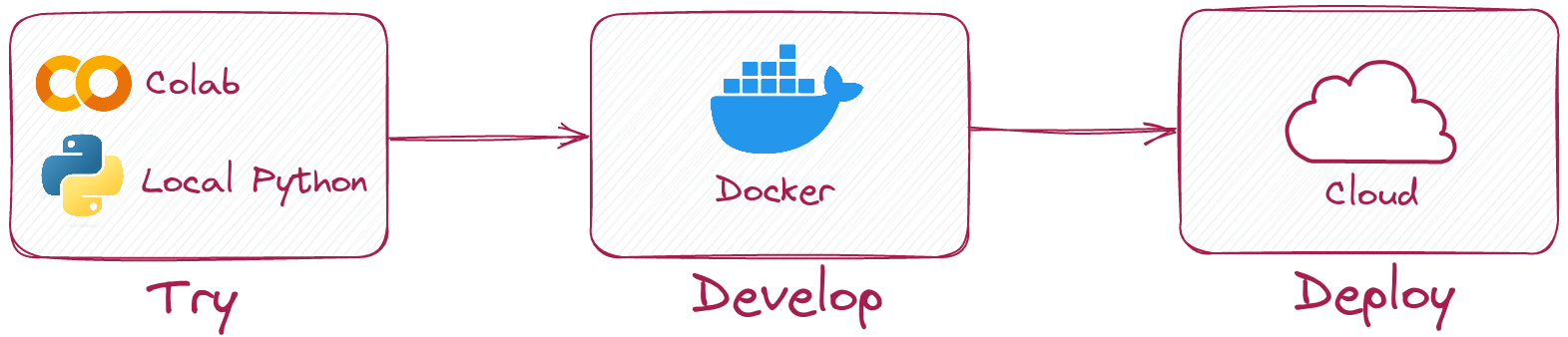
First, try Qdrant locally using the [Qdrant Client](https://github.com/qdrant/qdrant-client) and with the help of our [Tutorials](tutorials/) and Guides. Develop a sample app from our [Examples](examples/) list and try it using a [Qdrant Docker](guides/installation/) container. Then, when you are ready for production, deploy to a Free Tier [Qdrant Cloud](cloud/) cluster.
### Try Qdrant with Practice Data:
You may always use our [Practice Datasets](datasets/) to build with Qdrant. This page will be regularly updated with dataset snapshots you can use to bootstrap complete projects.
## Popular Topics:
| Tutorial | Description | Tutorial| Description |
|----------------------------------------------------|----------------------------------------------|---------|------------------|
| [Installation](guides/installation/) | Different ways to install Qdrant. | [Collections](concepts/collections/) | Learn about the central concept behind Qdrant. |
| [Configuration](guides/configuration/) | Update the default configuration. | [Bulk Upload](tutorials/bulk-upload/) | Efficiently upload a large number of vectors. |
| [Optimization](tutorials/optimize/) | Optimize Qdrant's resource usage. | [Multitenancy](tutorials/multiple-partitions/) | Setup Qdrant for multiple independent users. |
## Common Use Cases:
Qdrant is ideal for deploying applications based on the matching of embeddings produced by neural network encoders. Check out the [Examples](examples/) section to learn more about common use cases. Also, you can visit the [Tutorials](tutorials/) page to learn how to work with Qdrant in different ways.
| Use Case | Description | Stack |
|-----------------------|----------------------------------------------|--------|
| [Semantic Search for Beginners](tutorials/search-beginners/) | Build a search engine locally with our most basic instruction set. | Qdrant |
| [Build a Simple Neural Search](tutorials/neural-search/) | Build and deploy a neural search. [Check out the live demo app.](https://demo.qdrant.tech/#/) | Qdrant, BERT, FastAPI |
| [Build a Search with Aleph Alpha](tutorials/aleph-alpha-search/) | Build a simple semantic search that combines text and image data. | Qdrant, Aleph Alpha |
| [Developing Recommendations Systems](https://githubtocolab.com/qdrant/examples/blob/master/qdrant_101_getting_started/getting_started.ipynb) | Learn how to get started building semantic search and recommendation systems. | Qdrant |
| [Search and Recommend Newspaper Articles](https://githubtocolab.com/qdrant/examples/blob/master/qdrant_101_text_data/qdrant_and_text_data.ipynb) | Work with text data to develop a semantic search and a recommendation engine for news articles. | Qdrant |
| [Recommendation System for Songs](https://githubtocolab.com/qdrant/examples/blob/master/qdrant_101_audio_data/03_qdrant_101_audio.ipynb) | Use Qdrant to develop a music recommendation engine based on audio embeddings. | Qdrant |
| [Image Comparison System for Skin Conditions](https://colab.research.google.com/github/qdrant/examples/blob/master/qdrant_101_image_data/04_qdrant_101_cv.ipynb) | Use Qdrant to compare challenging images with labels representing different skin diseases. | Qdrant |
| [Question and Answer System with LlamaIndex](https://githubtocolab.com/qdrant/examples/blob/master/llama_index_recency/Qdrant%20and%20LlamaIndex%20%E2%80%94%20A%20new%20way%20to%20keep%20your%20Q%26A%20systems%20up-to-date.ipynb) | Combine Qdrant and LlamaIndex to create a self-updating Q&A system. | Qdrant, LlamaIndex, Cohere |
| [Extractive QA System](https://githubtocolab.com/qdrant/examples/blob/master/extractive_qa/extractive-question-answering.ipynb) | Extract answers directly from context to generate highly relevant answers. | Qdrant |
| [Ecommerce Reverse Image Search](https://githubtocolab.com/qdrant/examples/blob/master/ecommerce_reverse_image_search/ecommerce-reverse-image-search.ipynb) | Accept images as search queries to receive semantically appropriate answers. | Qdrant | ",documentation/_index.md
"---
title: Contribution Guidelines
weight: 35
draft: true
---
# How to contribute
If you are a Qdrant user - Data Scientist, ML Engineer, or MLOps, the best contribution would be the feedback on your experience with Qdrant.
Let us know whenever you have a problem, face an unexpected behavior, or see a lack of documentation.
You can do it in any convenient way - create an [issue](https://github.com/qdrant/qdrant/issues), start a [discussion](https://github.com/qdrant/qdrant/discussions), or drop up a [message](https://discord.gg/tdtYvXjC4h).
If you use Qdrant or Metric Learning in your projects, we'd love to hear your story! Feel free to share articles and demos in our community.
For those familiar with Rust - check out our [contribution guide](https://github.com/qdrant/qdrant/blob/master/CONTRIBUTING.md).
If you have problems with code or architecture understanding - reach us at any time.
Feeling confident and want to contribute more? - Come to [work with us](https://qdrant.join.com/)!",documentation/contribution-guidelines.md
"---
title: API Reference
weight: 20
type: external-link
external_url: https://qdrant.github.io/qdrant/redoc/index.html
sitemapExclude: True
---",documentation/api-reference.md
"---
title: OpenAI
weight: 800
aliases: [ ../integrations/openai/ ]
---
# OpenAI
Qdrant can also easily work with [OpenAI embeddings](https://platform.openai.com/docs/guides/embeddings/embeddings).
There is an official OpenAI Python package that simplifies obtaining them, and it might be installed with pip:
```bash
pip install openai
```
Once installed, the package exposes the method allowing to retrieve the embedding for given text. OpenAI requires an API key that has to be provided either as an environmental variable `OPENAI_API_KEY` or set in the source code directly, as presented below:
```python
import openai
import qdrant_client
from qdrant_client.http.models import Batch
# Choose one of the available models:
# https://platform.openai.com/docs/models/embeddings
embedding_model = ""text-embedding-ada-002""
openai_client = openai.Client(
api_key=""<< your_api_key >>""
)
response = openai_client.embeddings.create(
input=""The best vector database"",
model=embedding_model,
)
qdrant_client = qdrant_client.QdrantClient()
qdrant_client.upsert(
collection_name=""MyCollection"",
points=Batch(
ids=[1],
vectors=[response.data[0].embedding],
),
)
```
",documentation/embeddings/openai.md
"---
title: AWS Bedrock
weight: 1000
---
# Bedrock Embeddings
You can use [AWS Bedrock](https://aws.amazon.com/bedrock/) with Qdrant. AWS Bedrock supports multiple [embedding model providers](https://docs.aws.amazon.com/bedrock/latest/userguide/models-supported.html).
You'll need the following information from your AWS account:
- Region
- Access key ID
- Secret key
To configure your credentials, review the following AWS article: [How do I create an AWS access key](https://repost.aws/knowledge-center/create-access-key).
With the following code sample, you can generate embeddings using the [Titan Embeddings G1 - Text model](https://docs.aws.amazon.com/bedrock/latest/userguide/titan-embedding-models.html) which produces sentence embeddings of size 1536.
```python
# Install the required dependencies
# pip install boto3 qdrant_client
import json
import boto3
from qdrant_client import QdrantClient, models
session = boto3.Session()
bedrock_client = session.client(
""bedrock-runtime"",
region_name="""",
aws_access_key_id="""",
aws_secret_access_key="""",
)
qdrant_client = QdrantClient(location=""http://localhost:6333"")
qdrant_client.create_collection(
""{collection_name}"",
vectors_config=models.VectorParams(size=1536, distance=models.Distance.COSINE),
)
body = json.dumps({""inputText"": ""Some text to generate embeddings for""})
response = bedrock_client.invoke_model(
body=body,
modelId=""amazon.titan-embed-text-v1"",
accept=""application/json"",
contentType=""application/json"",
)
response_body = json.loads(response.get(""body"").read())
qdrant_client.upsert(
""{collection_name}"",
points=[models.PointStruct(id=1, vector=response_body[""embedding""])],
)
```
```javascript
// Install the required dependencies
// npm install @aws-sdk/client-bedrock-runtime @qdrant/js-client-rest
import {
BedrockRuntimeClient,
InvokeModelCommand,
} from ""@aws-sdk/client-bedrock-runtime"";
import { QdrantClient } from '@qdrant/js-client-rest';
const main = async () => {
const bedrockClient = new BedrockRuntimeClient({
region: """",
credentials: {
accessKeyId: """",,
secretAccessKey: """",
},
});
const qdrantClient = new QdrantClient({ url: 'http://localhost:6333' });
await qdrantClient.createCollection(""{collection_name}"", {
vectors: {
size: 1536,
distance: 'Cosine',
}
});
const response = await bedrockClient.send(
new InvokeModelCommand({
modelId: ""amazon.titan-embed-text-v1"",
body: JSON.stringify({
inputText: ""Some text to generate embeddings for"",
}),
contentType: ""application/json"",
accept: ""application/json"",
})
);
const body = new TextDecoder().decode(response.body);
await qdrantClient.upsert(""{collection_name}"", {
points: [
{
id: 1,
vector: JSON.parse(body).embedding,
},
],
});
}
main();
```
",documentation/embeddings/bedrock.md
"---
title: Aleph Alpha
weight: 900
aliases: [ ../integrations/aleph-alpha/ ]
---
Aleph Alpha is a multimodal and multilingual embeddings' provider. Their API allows creating the embeddings for text and images, both
in the same latent space. They maintain an [official Python client](https://github.com/Aleph-Alpha/aleph-alpha-client) that might be
installed with pip:
```bash
pip install aleph-alpha-client
```
There is both synchronous and asynchronous client available. Obtaining the embeddings for an image and storing it into Qdrant might
be done in the following way:
```python
import qdrant_client
from aleph_alpha_client import (
Prompt,
AsyncClient,
SemanticEmbeddingRequest,
SemanticRepresentation,
ImagePrompt
)
from qdrant_client.http.models import Batch
aa_token = ""<< your_token >>""
model = ""luminous-base""
qdrant_client = qdrant_client.QdrantClient()
async with AsyncClient(token=aa_token) as client:
prompt = ImagePrompt.from_file(""./path/to/the/image.jpg"")
prompt = Prompt.from_image(prompt)
query_params = {
""prompt"": prompt,
""representation"": SemanticRepresentation.Symmetric,
""compress_to_size"": 128,
}
query_request = SemanticEmbeddingRequest(**query_params)
query_response = await client.semantic_embed(
request=query_request, model=model
)
qdrant_client.upsert(
collection_name=""MyCollection"",
points=Batch(
ids=[1],
vectors=[query_response.embedding],
)
)
```
If we wanted to create text embeddings with the same model, we wouldn't use `ImagePrompt.from_file`, but simply provide the input
text into the `Prompt.from_text` method.
",documentation/embeddings/aleph-alpha.md
"---
title: Cohere
weight: 700
aliases: [ ../integrations/cohere/ ]
---
# Cohere
Qdrant is compatible with Cohere [co.embed API](https://docs.cohere.ai/reference/embed) and its official Python SDK that
might be installed as any other package:
```bash
pip install cohere
```
The embeddings returned by co.embed API might be used directly in the Qdrant client's calls:
```python
import cohere
import qdrant_client
from qdrant_client.http.models import Batch
cohere_client = cohere.Client(""<< your_api_key >>"")
qdrant_client = qdrant_client.QdrantClient()
qdrant_client.upsert(
collection_name=""MyCollection"",
points=Batch(
ids=[1],
vectors=cohere_client.embed(
model=""large"",
texts=[""The best vector database""],
).embeddings,
),
)
```
If you are interested in seeing an end-to-end project created with co.embed API and Qdrant, please check out the
""[Question Answering as a Service with Cohere and Qdrant](https://qdrant.tech/articles/qa-with-cohere-and-qdrant/)"" article.
## Embed v3
Embed v3 is a new family of Cohere models, released in November 2023. The new models require passing an additional
parameter to the API call: `input_type`. It determines the type of task you want to use the embeddings for.
- `input_type=""search_document""` - for documents to store in Qdrant
- `input_type=""search_query""` - for search queries to find the most relevant documents
- `input_type=""classification""` - for classification tasks
- `input_type=""clustering""` - for text clustering
While implementing semantic search applications, such as RAG, you should use `input_type=""search_document""` for the
indexed documents and `input_type=""search_query""` for the search queries. The following example shows how to index
documents with the Embed v3 model:
```python
import cohere
import qdrant_client
from qdrant_client.http.models import Batch
cohere_client = cohere.Client(""<< your_api_key >>"")
qdrant_client = qdrant_client.QdrantClient()
qdrant_client.upsert(
collection_name=""MyCollection"",
points=Batch(
ids=[1],
vectors=cohere_client.embed(
model=""embed-english-v3.0"", # New Embed v3 model
input_type=""search_document"", # Input type for documents
texts=[""Qdrant is the a vector database written in Rust""],
).embeddings,
),
)
```
Once the documents are indexed, you can search for the most relevant documents using the Embed v3 model:
```python
qdrant_client.search(
collection_name=""MyCollection"",
query=cohere_client.embed(
model=""embed-english-v3.0"", # New Embed v3 model
input_type=""search_query"", # Input type for search queries
texts=[""The best vector database""],
).embeddings[0],
)
```
",documentation/embeddings/cohere.md
"---
title: ""Nomic""
weight: 1100
---
# Nomic
The `nomic-embed-text-v1` model is an open source [8192 context length](https://github.com/nomic-ai/contrastors) text encoder.
While you can find it on the [Hugging Face Hub](https://huggingface.co/nomic-ai/nomic-embed-text-v1),
you may find it easier to obtain them through the [Nomic Text Embeddings](https://docs.nomic.ai/reference/endpoints/nomic-embed-text).
Once installed, you can configure it with the official Python client or through direct HTTP requests.
You can use Nomic embeddings directly in Qdrant client calls. There is a difference in the way the embeddings
are obtained for documents and queries. The `task_type` parameter defines the embeddings that you get.
For documents, set the `task_type` to `search_document`:
```python
from qdrant_client import QdrantClient, models
from nomic import embed
output = embed.text(
texts=[""Qdrant is the best vector database!""],
model=""nomic-embed-text-v1"",
task_type=""search_document"",
)
qdrant_client = QdrantClient()
qdrant_client.upsert(
collection_name=""my-collection"",
points=models.Batch(
ids=[1],
vectors=output[""embeddings""],
),
)
```
To query the collection, set the `task_type` to `search_query`:
```python
output = embed.text(
texts=[""What is the best vector database?""],
model=""nomic-embed-text-v1"",
task_type=""search_query"",
)
qdrant_client.search(
collection_name=""my-collection"",
query=output[""embeddings""][0],
)
```
For more information, see the Nomic documentation on [Text embeddings](https://docs.nomic.ai/reference/endpoints/nomic-embed-text).
",documentation/embeddings/nomic.md
"---
title: Gemini
weight: 700
---
# Gemini
Qdrant is compatible with Gemini Embedding Model API and its official Python SDK that can be installed as any other package:
Gemini is a new family of Google PaLM models, released in December 2023. The new embedding models succeed the previous Gecko Embedding Model.
In the latest models, an additional parameter, `task_type`, can be passed to the API call. This parameter serves to designate the intended purpose for the embeddings utilized.
The Embedding Model API supports various task types, outlined as follows:
1. `retrieval_query`: Specifies the given text is a query in a search/retrieval setting.
2. `retrieval_document`: Specifies the given text is a document from the corpus being searched.
3. `semantic_similarity`: Specifies the given text will be used for Semantic Text Similarity.
4. `classification`: Specifies that the given text will be classified.
5. `clustering`: Specifies that the embeddings will be used for clustering.
6. `task_type_unspecified`: Unset value, which will default to one of the other values.
If you're building a semantic search application, such as RAG, you should use `task_type=""retrieval_document""` for the indexed documents and `task_type=""retrieval_query""` for the search queries.
The following example shows how to do this with Qdrant:
## Setup
```bash
pip install google-generativeai
```
Let's see how to use the Embedding Model API to embed a document for retrieval.
The following example shows how to embed a document with the `models/embedding-001` with the `retrieval_document` task type:
## Embedding a document
```python
import pathlib
import google.generativeai as genai
import qdrant_client
GEMINI_API_KEY = ""YOUR GEMINI API KEY"" # add your key here
genai.configure(api_key=GEMINI_API_KEY)
result = genai.embed_content(
model=""models/embedding-001"",
content=""Qdrant is the best vector search engine to use with Gemini"",
task_type=""retrieval_document"",
title=""Qdrant x Gemini"",
)
```
The returned result is a dictionary with a key: `embedding`. The value of this key is a list of floats representing the embedding of the document.
## Indexing documents with Qdrant
```python
from qdrant_client.http.models import Batch
qdrant_client = qdrant_client.QdrantClient()
qdrant_client.upsert(
collection_name=""GeminiCollection"",
points=Batch(
ids=[1],
vectors=genai.embed_content(
model=""models/embedding-001"",
content=""Qdrant is the best vector search engine to use with Gemini"",
task_type=""retrieval_document"",
title=""Qdrant x Gemini"",
)[""embedding""],
),
)
```
## Searching for documents with Qdrant
Once the documents are indexed, you can search for the most relevant documents using the same model with the `retrieval_query` task type:
```python
qdrant_client.search(
collection_name=""GeminiCollection"",
query=genai.embed_content(
model=""models/embedding-001"",
content=""What is the best vector database to use with Gemini?"",
task_type=""retrieval_query"",
)[""embedding""],
)
```
## Using Gemini Embedding Models with Binary Quantization
You can use Gemini Embedding Models with [Binary Quantization](/articles/binary-quantization/) - a technique that allows you to reduce the size of the embeddings by 32 times without losing the quality of the search results too much.
In this table, you can see the results of the search with the `models/embedding-001` model with Binary Quantization in comparison with the original model:
At an oversampling of 3 and a limit of 100, we've a 95% recall against the exact nearest neighbors with rescore enabled.
| oversampling | | 1 | 1 | 2 | 2 | 3 | 3 |
|--------------|---------|----------|----------|----------|----------|----------|----------|
| limit | | | | | | | |
| | rescore | False | True | False | True | False | True |
| 10 | | 0.523333 | 0.831111 | 0.523333 | 0.915556 | 0.523333 | 0.950000 |
| 20 | | 0.510000 | 0.836667 | 0.510000 | 0.912222 | 0.510000 | 0.937778 |
| 50 | | 0.489111 | 0.841556 | 0.489111 | 0.913333 | 0.488444 | 0.947111 |
| 100 | | 0.485778 | 0.846556 | 0.485556 | 0.929000 | 0.486000 | **0.956333** |
That's it! You can now use Gemini Embedding Models with Qdrant!",documentation/embeddings/gemini.md
"---
title: Jina Embeddings
weight: 800
aliases: [ ../integrations/jina-embeddings/ ]
---
# Jina Embeddings
Qdrant can also easily work with [Jina embeddings](https://jina.ai/embeddings/) which allow for model input lengths of up to 8192 tokens.
To call their endpoint, all you need is an API key obtainable [here](https://jina.ai/embeddings/). By the way, our friends from **Jina AI** provided us with a code (**QDRANT**) that will grant you a **10% discount** if you plan to use Jina Embeddings in production.
```python
import qdrant_client
import requests
from qdrant_client.http.models import Distance, VectorParams
from qdrant_client.http.models import Batch
# Provide Jina API key and choose one of the available models.
# You can get a free trial key here: https://jina.ai/embeddings/
JINA_API_KEY = ""jina_xxxxxxxxxxx""
MODEL = ""jina-embeddings-v2-base-en"" # or ""jina-embeddings-v2-base-en""
EMBEDDING_SIZE = 768 # 512 for small variant
# Get embeddings from the API
url = ""https://api.jina.ai/v1/embeddings""
headers = {
""Content-Type"": ""application/json"",
""Authorization"": f""Bearer {JINA_API_KEY}"",
}
data = {
""input"": [""Your text string goes here"", ""You can send multiple texts""],
""model"": MODEL,
}
response = requests.post(url, headers=headers, json=data)
embeddings = [d[""embedding""] for d in response.json()[""data""]]
# Index the embeddings into Qdrant
qdrant_client = qdrant_client.QdrantClient("":memory:"")
qdrant_client.create_collection(
collection_name=""MyCollection"",
vectors_config=VectorParams(size=EMBEDDING_SIZE, distance=Distance.DOT),
)
qdrant_client.upsert(
collection_name=""MyCollection"",
points=Batch(
ids=list(range(len(embeddings))),
vectors=embeddings,
),
)
```
",documentation/embeddings/jina-embeddings.md
"---
title: Embeddings
weight: 33
# If the index.md file is empty, the link to the section will be hidden from the sidebar
is_empty: true
---
| Embedding |
|---|
| [Gemini](./gemini/) |
| [Aleph Alpha](./aleph-alpha/) |
| [Cohere](./cohere/) |
| [Jina](./jina-emebddngs/) |
| [OpenAI](./openai/) |",documentation/embeddings/_index.md
"---
title: Database Optimization
weight: 3
---
## Database Optimization Strategies
### How do I reduce memory usage?
The primary source of memory usage vector data. There are several ways to address that:
- Configure [Quantization](../../guides/quantization/) to reduce the memory usage of vectors.
- Configure on-disk vector storage
The choice of the approach depends on your requirements.
Read more about [configuring the optimal](../../tutorials/optimize/) use of Qdrant.
### How do you choose machine configuration?
There are two main scenarios of Qdrant usage in terms of resource consumption:
- **Performance-optimized** -- when you need to serve vector search as fast (many) as possible. In this case, you need to have as much vector data in RAM as possible. Use our [calculator](https://cloud.qdrant.io/calculator) to estimate the required RAM.
- **Storage-optimized** -- when you need to store many vectors and minimize costs by compromising some search speed. In this case, pay attention to the disk speed instead. More about it in the article about [Memory Consumption](../../../articles/memory-consumption/).
### I configured on-disk vector storage, but memory usage is still high. Why?
Firstly, memory usage metrics as reported by `top` or `htop` may be misleading. They are not showing the minimal amount of memory required to run the service.
If the RSS memory usage is 10 GB, it doesn't mean that it won't work on a machine with 8 GB of RAM.
Qdrant uses many techniques to reduce search latency, including caching disk data in RAM and preloading data from disk to RAM.
As a result, the Qdrant process might use more memory than the minimum required to run the service.
> Unused RAM is wasted RAM
If you want to limit the memory usage of the service, we recommend using [limits in Docker](https://docs.docker.com/config/containers/resource_constraints/#memory) or Kubernetes.
### My requests are very slow or time out. What should I do?
There are several possible reasons for that:
- **Using filters without payload index** -- If you're performing a search with a filter but you don't have a payload index, Qdrant will have to load whole payload data from disk to check the filtering condition. Ensure you have adequately configured [payload indexes](../../concepts/indexing/#payload-index).
- **Usage of on-disk vector storage with slow disks** -- If you're using on-disk vector storage, ensure you have fast enough disks. We recommend using local SSDs with at least 50k IOPS. Read more about the influence of the disk speed on the search latency in the article about [Memory Consumption](../../../articles/memory-consumption/).
- **Large limit or non-optimal query parameters** -- A large limit or offset might lead to significant performance degradation. Please pay close attention to the query/collection parameters that significantly diverge from the defaults. They might be the reason for the performance issues.
",documentation/faq/database-optimization.md
"---
title: Fundamentals
weight: 1
---
## Qdrant Fundamentals
### How many collections can I create?
As much as you want, but be aware that each collection requires additional resources.
It is _highly_ recommended not to create many small collections, as it will lead to significant resource consumption overhead.
We consider creating a collection for each user/dialog/document as an antipattern.
Please read more about collections, isolation, and multiple users in our [Multitenancy](../../tutorials/multiple-partitions/) tutorial.
### My search results contain vectors with null values. Why?
By default, Qdrant tries to minimize network traffic and doesn't return vectors in search results.
But you can force Qdrant to do so by setting the `with_vector` parameter of the Search/Scroll to `true`.
If you're still seeing `""vector"": null` in your results, it might be that the vector you're passing is not in the correct format, or there's an issue with how you're calling the upsert method.
### How can I search without a vector?
You are likely looking for the [scroll](../../concepts/points/#scroll-points) method. It allows you to retrieve the records based on filters or even iterate over all the records in the collection.
### Does Qdrant support a full-text search or a hybrid search?
Qdrant is a vector search engine in the first place, and we only implement full-text support as long as it doesn't compromise the vector search use case.
That includes both the interface and the performance.
What Qdrant can do:
- Search with full-text filters
- Apply full-text filters to the vector search (i.e., perform vector search among the records with specific words or phrases)
- Do prefix search and semantic [search-as-you-type](../../../articles/search-as-you-type/)
What Qdrant plans to introduce in the future:
- Support for sparse vectors, as used in [SPLADE](https://github.com/naver/splade) or similar models
What Qdrant doesn't plan to support:
- BM25 or other non-vector-based retrieval or ranking functions
- Built-in ontologies or knowledge graphs
- Query analyzers and other NLP tools
Of course, you can always combine Qdrant with any specialized tool you need, including full-text search engines.
Read more about [our approach](../../../articles/hybrid-search/) to hybrid search.
### How do I upload a large number of vectors into a Qdrant collection?
Read about our recommendations in the [bulk upload](../../tutorials/bulk-upload/) tutorial.
### Can I only store quantized vectors and discard full precision vectors?
No, Qdrant requires full precision vectors for operations like reindexing, rescoring, etc.
## Qdrant Cloud
### Is it possible to scale down a Qdrant Cloud cluster?
In general, no. There's no way to scale down the underlying disk storage.
But in some cases, we might be able to help you with that through manual intervention, but it's not guaranteed.
## Versioning
### How do I avoid issues when updating to the latest version?
We only guarantee compatibility if you update between consequent versions. You would need to upgrade versions one at a time: `1.1 -> 1.2`, then `1.2 -> 1.3`, then `1.3 -> 1.4`.
### Do you guarantee compatibility across versions?
In case your version is older, we guarantee only compatibility between two consecutive minor versions.
While we will assist with break/fix troubleshooting of issues and errors specific to our products, Qdrant is not accountable for reviewing, writing (or rewriting), or debugging custom code.
",documentation/faq/qdrant-fundamentals.md
"---
title: FAQ
weight: 41
is_empty: true
---",documentation/faq/_index.md
"---
title: Multitenancy
weight: 12
aliases:
- ../tutorials/multiple-partitions
---
# Configure Multitenancy
**How many collections should you create?** In most cases, you should only use a single collection with payload-based partitioning. This approach is called multitenancy. It is efficient for most of users, but it requires additional configuration. This document will show you how to set it up.
**When should you create multiple collections?** When you have a limited number of users and you need isolation. This approach is flexible, but it may be more costly, since creating numerous collections may result in resource overhead. Also, you need to ensure that they do not affect each other in any way, including performance-wise.
## Partition by payload
When an instance is shared between multiple users, you may need to partition vectors by user. This is done so that each user can only access their own vectors and can't see the vectors of other users.
1. Add a `group_id` field to each vector in the collection.
```http
PUT /collections/{collection_name}/points
{
""points"": [
{
""id"": 1,
""payload"": {""group_id"": ""user_1""},
""vector"": [0.9, 0.1, 0.1]
},
{
""id"": 2,
""payload"": {""group_id"": ""user_1""},
""vector"": [0.1, 0.9, 0.1]
},
{
""id"": 3,
""payload"": {""group_id"": ""user_2""},
""vector"": [0.1, 0.1, 0.9]
},
]
}
```
```python
client.upsert(
collection_name=""{collection_name}"",
points=[
models.PointStruct(
id=1,
payload={""group_id"": ""user_1""},
vector=[0.9, 0.1, 0.1],
),
models.PointStruct(
id=2,
payload={""group_id"": ""user_1""},
vector=[0.1, 0.9, 0.1],
),
models.PointStruct(
id=3,
payload={""group_id"": ""user_2""},
vector=[0.1, 0.1, 0.9],
),
],
)
```
```typescript
import { QdrantClient } from ""@qdrant/js-client-rest"";
const client = new QdrantClient({ host: ""localhost"", port: 6333 });
client.upsert(""{collection_name}"", {
points: [
{
id: 1,
payload: { group_id: ""user_1"" },
vector: [0.9, 0.1, 0.1],
},
{
id: 2,
payload: { group_id: ""user_1"" },
vector: [0.1, 0.9, 0.1],
},
{
id: 3,
payload: { group_id: ""user_2"" },
vector: [0.1, 0.1, 0.9],
},
],
});
```
```rust
use qdrant_client::{client::QdrantClient, qdrant::PointStruct};
use serde_json::json;
let client = QdrantClient::from_url(""http://localhost:6334"").build()?;
client
.upsert_points_blocking(
""{collection_name}"".to_string(),
None,
vec![
PointStruct::new(
1,
vec![0.9, 0.1, 0.1],
json!(
{""group_id"": ""user_1""}
)
.try_into()
.unwrap(),
),
PointStruct::new(
2,
vec![0.1, 0.9, 0.1],
json!(
{""group_id"": ""user_1""}
)
.try_into()
.unwrap(),
),
PointStruct::new(
3,
vec![0.1, 0.1, 0.9],
json!(
{""group_id"": ""user_2""}
)
.try_into()
.unwrap(),
),
],
None,
)
.await?;
```
```java
import java.util.List;
import java.util.Map;
import io.qdrant.client.QdrantClient;
import io.qdrant.client.QdrantGrpcClient;
import io.qdrant.client.grpc.Points.PointStruct;
QdrantClient client =
new QdrantClient(QdrantGrpcClient.newBuilder(""localhost"", 6334, false).build());
client
.upsertAsync(
""{collection_name}"",
List.of(
PointStruct.newBuilder()
.setId(id(1))
.setVectors(vectors(0.9f, 0.1f, 0.1f))
.putAllPayload(Map.of(""group_id"", value(""user_1"")))
.build(),
PointStruct.newBuilder()
.setId(id(2))
.setVectors(vectors(0.1f, 0.9f, 0.1f))
.putAllPayload(Map.of(""group_id"", value(""user_1"")))
.build(),
PointStruct.newBuilder()
.setId(id(3))
.setVectors(vectors(0.1f, 0.1f, 0.9f))
.putAllPayload(Map.of(""group_id"", value(""user_2"")))
.build()))
.get();
```
```csharp
using Qdrant.Client;
using Qdrant.Client.Grpc;
var client = new QdrantClient(""localhost"", 6334);
await client.UpsertAsync(
collectionName: ""{collection_name}"",
points: new List
{
new()
{
Id = 1,
Vectors = new[] { 0.9f, 0.1f, 0.1f },
Payload = { [""group_id""] = ""user_1"" }
},
new()
{
Id = 2,
Vectors = new[] { 0.1f, 0.9f, 0.1f },
Payload = { [""group_id""] = ""user_1"" }
},
new()
{
Id = 3,
Vectors = new[] { 0.1f, 0.1f, 0.9f },
Payload = { [""group_id""] = ""user_2"" }
}
}
);
```
2. Use a filter along with `group_id` to filter vectors for each user.
```http
POST /collections/{collection_name}/points/search
{
""filter"": {
""must"": [
{
""key"": ""group_id"",
""match"": {
""value"": ""user_1""
}
}
]
},
""vector"": [0.1, 0.1, 0.9],
""limit"": 10
}
```
```python
from qdrant_client import QdrantClient, models
client = QdrantClient(""localhost"", port=6333)
client.search(
collection_name=""{collection_name}"",
query_filter=models.Filter(
must=[
models.FieldCondition(
key=""group_id"",
match=models.MatchValue(
value=""user_1"",
),
)
]
),
query_vector=[0.1, 0.1, 0.9],
limit=10,
)
```
```typescript
import { QdrantClient } from ""@qdrant/js-client-rest"";
const client = new QdrantClient({ host: ""localhost"", port: 6333 });
client.search(""{collection_name}"", {
filter: {
must: [{ key: ""group_id"", match: { value: ""user_1"" } }],
},
vector: [0.1, 0.1, 0.9],
limit: 10,
});
```
```rust
use qdrant_client::{
client::QdrantClient,
qdrant::{Condition, Filter, SearchPoints},
};
let client = QdrantClient::from_url(""http://localhost:6334"").build()?;
client
.search_points(&SearchPoints {
collection_name: ""{collection_name}"".to_string(),
filter: Some(Filter::must([Condition::matches(
""group_id"",
""user_1"".to_string(),
)])),
vector: vec![0.1, 0.1, 0.9],
limit: 10,
..Default::default()
})
.await?;
```
```java
import java.util.List;
import io.qdrant.client.QdrantClient;
import io.qdrant.client.QdrantGrpcClient;
import io.qdrant.client.grpc.Points.Filter;
import io.qdrant.client.grpc.Points.SearchPoints;
QdrantClient client =
new QdrantClient(QdrantGrpcClient.newBuilder(""localhost"", 6334, false).build());
client
.searchAsync(
SearchPoints.newBuilder()
.setCollectionName(""{collection_name}"")
.setFilter(
Filter.newBuilder().addMust(matchKeyword(""group_id"", ""user_1"")).build())
.addAllVector(List.of(0.1f, 0.1f, 0.9f))
.setLimit(10)
.build())
.get();
```
```csharp
using Qdrant.Client;
using Qdrant.Client.Grpc;
using static Qdrant.Client.Grpc.Conditions;
var client = new QdrantClient(""localhost"", 6334);
await client.SearchAsync(
collectionName: ""{collection_name}"",
vector: new float[] { 0.1f, 0.1f, 0.9f },
filter: MatchKeyword(""group_id"", ""user_1""),
limit: 10
);
```
## Calibrate performance
The speed of indexation may become a bottleneck in this case, as each user's vector will be indexed into the same collection. To avoid this bottleneck, consider _bypassing the construction of a global vector index_ for the entire collection and building it only for individual groups instead.
By adopting this strategy, Qdrant will index vectors for each user independently, significantly accelerating the process.
To implement this approach, you should:
1. Set `payload_m` in the HNSW configuration to a non-zero value, such as 16.
2. Set `m` in hnsw config to 0. This will disable building global index for the whole collection.
```http
PUT /collections/{collection_name}
{
""vectors"": {
""size"": 768,
""distance"": ""Cosine""
},
""hnsw_config"": {
""payload_m"": 16,
""m"": 0
}
}
```
```python
from qdrant_client import QdrantClient, models
client = QdrantClient(""localhost"", port=6333)
client.create_collection(
collection_name=""{collection_name}"",
vectors_config=models.VectorParams(size=768, distance=models.Distance.COSINE),
hnsw_config=models.HnswConfigDiff(
payload_m=16,
m=0,
),
)
```
```typescript
import { QdrantClient } from ""@qdrant/js-client-rest"";
const client = new QdrantClient({ host: ""localhost"", port: 6333 });
client.createCollection(""{collection_name}"", {
vectors: {
size: 768,
distance: ""Cosine"",
},
hnsw_config: {
payload_m: 16,
m: 0,
},
});
```
```rust
use qdrant_client::{
client::QdrantClient,
qdrant::{
vectors_config::Config, CreateCollection, Distance, HnswConfigDiff, VectorParams,
VectorsConfig,
},
};
let client = QdrantClient::from_url(""http://localhost:6334"").build()?;
client
.create_collection(&CreateCollection {
collection_name: ""{collection_name}"".to_string(),
vectors_config: Some(VectorsConfig {
config: Some(Config::Params(VectorParams {
size: 768,
distance: Distance::Cosine.into(),
..Default::default()
})),
}),
hnsw_config: Some(HnswConfigDiff {
payload_m: Some(16),
m: Some(0),
..Default::default()
}),
..Default::default()
})
.await?;
```
```java
import io.qdrant.client.QdrantClient;
import io.qdrant.client.QdrantGrpcClient;
import io.qdrant.client.grpc.Collections.CreateCollection;
import io.qdrant.client.grpc.Collections.Distance;
import io.qdrant.client.grpc.Collections.HnswConfigDiff;
import io.qdrant.client.grpc.Collections.VectorParams;
import io.qdrant.client.grpc.Collections.VectorsConfig;
QdrantClient client =
new QdrantClient(QdrantGrpcClient.newBuilder(""localhost"", 6334, false).build());
client
.createCollectionAsync(
CreateCollection.newBuilder()
.setCollectionName(""{collection_name}"")
.setVectorsConfig(
VectorsConfig.newBuilder()
.setParams(
VectorParams.newBuilder()
.setSize(768)
.setDistance(Distance.Cosine)
.build())
.build())
.setHnswConfig(HnswConfigDiff.newBuilder().setPayloadM(16).setM(0).build())
.build())
.get();
```
```csharp
using Qdrant.Client;
using Qdrant.Client.Grpc;
var client = new QdrantClient(""localhost"", 6334);
await client.CreateCollectionAsync(
collectionName: ""{collection_name}"",
vectorsConfig: new VectorParams { Size = 768, Distance = Distance.Cosine },
hnswConfig: new HnswConfigDiff { PayloadM = 16, M = 0 }
);
```
3. Create keyword payload index for `group_id` field.
```http
PUT /collections/{collection_name}/index
{
""field_name"": ""group_id"",
""field_schema"": ""keyword""
}
```
```python
client.create_payload_index(
collection_name=""{collection_name}"",
field_name=""group_id"",
field_schema=models.PayloadSchemaType.KEYWORD,
)
```
```typescript
client.createPayloadIndex(""{collection_name}"", {
field_name: ""group_id"",
field_schema: ""keyword"",
});
```
```rust
use qdrant_client::{client::QdrantClient, qdrant::FieldType};
let client = QdrantClient::from_url(""http://localhost:6334"").build()?;
client
.create_field_index(
""{collection_name}"",
""group_id"",
FieldType::Keyword,
None,
None,
)
.await?;
```
```java
import io.qdrant.client.QdrantClient;
import io.qdrant.client.QdrantGrpcClient;
import io.qdrant.client.grpc.Collections.PayloadSchemaType;
QdrantClient client =
new QdrantClient(QdrantGrpcClient.newBuilder(""localhost"", 6334, false).build());
client
.createPayloadIndexAsync(
""{collection_name}"", ""group_id"", PayloadSchsemaType.Keyword, null, null, null, null)
.get();
```
```csharp
using Qdrant.Client;
var client = new QdrantClient(""localhost"", 6334);
await client.CreatePayloadIndexAsync(collectionName: ""{collection_name}"", fieldName: ""group_id"");
```
## Limitations
One downside to this approach is that global requests (without the `group_id` filter) will be slower since they will necessitate scanning all groups to identify the nearest neighbors.
",documentation/guides/multiple-partitions.md
"---
title: Administration
weight: 10
aliases:
- ../administration
---
# Administration
Qdrant exposes administration tools which enable to modify at runtime the behavior of a qdrant instance without changing its configuration manually.
## Locking
A locking API enables users to restrict the possible operations on a qdrant process.
It is important to mention that:
- The configuration is not persistent therefore it is necessary to lock again following a restart.
- Locking applies to a single node only. It is necessary to call lock on all the desired nodes in a distributed deployment setup.
Lock request sample:
```http
POST /locks
{
""error_message"": ""write is forbidden"",
""write"": true
}
```
Write flags enables/disables write lock.
If the write lock is set to true, qdrant doesn't allow creating new collections or adding new data to the existing storage.
However, deletion operations or updates are not forbidden under the write lock.
This feature enables administrators to prevent a qdrant process from using more disk space while permitting users to search and delete unnecessary data.
You can optionally provide the error message that should be used for error responses to users.
## Recovery mode
*Available as of v1.2.0*
Recovery mode can help in situations where Qdrant fails to start repeatedly.
When starting in recovery mode, Qdrant only loads collection metadata to prevent
going out of memory. This allows you to resolve out of memory situations, for
example, by deleting a collection. After resolving Qdrant can be restarted
normally to continue operation.
In recovery mode, collection operations are limited to
[deleting](../../concepts/collections/#delete-collection) a
collection. That is because only collection metadata is loaded during recovery.
To enable recovery mode with the Qdrant Docker image you must set the
environment variable `QDRANT_ALLOW_RECOVERY_MODE=true`. The container will try
to start normally first, and restarts in recovery mode if initialisation fails
due to an out of memory error. This behavior is disabled by default.
If using a Qdrant binary, recovery mode can be enabled by setting a recovery
message in an environment variable, such as
`QDRANT__STORAGE__RECOVERY_MODE=""My recovery message""`.
",documentation/guides/administration.md
"---
title: Troubleshooting
weight: 170
aliases:
- ../tutorials/common-errors
---
# Solving common errors
## Too many files open (OS error 24)
Each collection segment needs some files to be open. At some point you may encounter the following errors in your server log:
```text
Error: Too many files open (OS error 24)
```
In such a case you may need to increase the limit of the open files. It might be done, for example, while you launch the Docker container:
```bash
docker run --ulimit nofile=10000:10000 qdrant/qdrant:latest
```
The command above will set both soft and hard limits to `10000`.
If you are not using Docker, the following command will change the limit for the current user session:
```bash
ulimit -n 10000
```
Please note, the command should be executed before you run Qdrant server.
",documentation/guides/common-errors.md
"---
title: Configuration
weight: 160
aliases:
- ../configuration
---
# Configuration
To change or correct Qdrant's behavior, default collection settings, and network interface parameters, you can use configuration files.
The default configuration file is located at [config/config.yaml](https://github.com/qdrant/qdrant/blob/master/config/config.yaml).
To change the default configuration, add a new configuration file and specify
the path with `--config-path path/to/custom_config.yaml`. If running in
production mode, you could also choose to overwrite `config/production.yaml`.
See [ordering](#order-and-priority) for details on how configurations are
loaded.
The [Installation](../installation) guide contains examples of how to set up Qdrant with a custom configuration for the different deployment methods.
## Order and priority
*Effective as of v1.2.1*
Multiple configurations may be loaded on startup. All of them are merged into a
single effective configuration that is used by Qdrant.
Configurations are loaded in the following order, if present:
1. Embedded base configuration ([source](https://github.com/qdrant/qdrant/blob/master/config/config.yaml))
2. File `config/config.yaml`
3. File `config/{RUN_MODE}.yaml` (such as `config/production.yaml`)
4. File `config/local.yaml`
5. Config provided with `--config-path PATH` (if set)
6. [Environment variables](#environment-variables)
This list is from least to most significant. Properties in later configurations
will overwrite those loaded before it. For example, a property set with
`--config-path` will overwrite those in other files.
Most of these files are included by default in the Docker container. But it is
likely that they are absent on your local machine if you run the `qdrant` binary
manually.
If file 2 or 3 are not found, a warning is shown on startup.
If file 5 is provided but not found, an error is shown on startup.
Other supported configuration file formats and extensions include: `.toml`, `.json`, `.ini`.
## Environment variables
It is possible to set configuration properties using environment variables.
Environment variables are always the most significant and cannot be overwritten
(see [ordering](#order-and-priority)).
All environment variables are prefixed with `QDRANT__` and are separated with
`__`.
These variables:
```bash
QDRANT__LOG_LEVEL=INFO
QDRANT__SERVICE__HTTP_PORT=6333
QDRANT__SERVICE__ENABLE_TLS=1
QDRANT__TLS__CERT=./tls/cert.pem
QDRANT__TLS__CERT_TTL=3600
```
result in this configuration:
```yaml
log_level: INFO
service:
http_port: 6333
enable_tls: true
tls:
cert: ./tls/cert.pem
cert_ttl: 3600
```
To run Qdrant locally with a different HTTP port you could use:
```bash
QDRANT__SERVICE__HTTP_PORT=1234 ./qdrant
```
## Configuration file example
```yaml
log_level: INFO
storage:
# Where to store all the data
storage_path: ./storage
# Where to store snapshots
snapshots_path: ./snapshots
# Where to store temporary files
# If null, temporary snapshot are stored in: storage/snapshots_temp/
temp_path: null
# If true - point's payload will not be stored in memory.
# It will be read from the disk every time it is requested.
# This setting saves RAM by (slightly) increasing the response time.
# Note: those payload values that are involved in filtering and are indexed - remain in RAM.
on_disk_payload: true
# Maximum number of concurrent updates to shard replicas
# If `null` - maximum concurrency is used.
update_concurrency: null
# Write-ahead-log related configuration
wal:
# Size of a single WAL segment
wal_capacity_mb: 32
# Number of WAL segments to create ahead of actual data requirement
wal_segments_ahead: 0
# Normal node - receives all updates and answers all queries
node_type: ""Normal""
# Listener node - receives all updates, but does not answer search/read queries
# Useful for setting up a dedicated backup node
# node_type: ""Listener""
performance:
# Number of parallel threads used for search operations. If 0 - auto selection.
max_search_threads: 0
# Max total number of threads, which can be used for running optimization processes across all collections.
# Note: Each optimization thread will also use `max_indexing_threads` for index building.
# So total number of threads used for optimization will be `max_optimization_threads * max_indexing_threads`
max_optimization_threads: 1
# Prevent DDoS of too many concurrent updates in distributed mode.
# One external update usually triggers multiple internal updates, which breaks internal
# timings. For example, the health check timing and consensus timing.
# If null - auto selection.
update_rate_limit: null
optimizers:
# The minimal fraction of deleted vectors in a segment, required to perform segment optimization
deleted_threshold: 0.2
# The minimal number of vectors in a segment, required to perform segment optimization
vacuum_min_vector_number: 1000
# Target amount of segments optimizer will try to keep.
# Real amount of segments may vary depending on multiple parameters:
# - Amount of stored points
# - Current write RPS
#
# It is recommended to select default number of segments as a factor of the number of search threads,
# so that each segment would be handled evenly by one of the threads.
# If `default_segment_number = 0`, will be automatically selected by the number of available CPUs
default_segment_number: 0
# Do not create segments larger this size (in KiloBytes).
# Large segments might require disproportionately long indexation times,
# therefore it makes sense to limit the size of segments.
#
# If indexation speed have more priority for your - make this parameter lower.
# If search speed is more important - make this parameter higher.
# Note: 1Kb = 1 vector of size 256
# If not set, will be automatically selected considering the number of available CPUs.
max_segment_size_kb: null
# Maximum size (in KiloBytes) of vectors to store in-memory per segment.
# Segments larger than this threshold will be stored as read-only memmaped file.
# To enable memmap storage, lower the threshold
# Note: 1Kb = 1 vector of size 256
# To explicitly disable mmap optimization, set to `0`.
# If not set, will be disabled by default.
memmap_threshold_kb: null
# Maximum size (in KiloBytes) of vectors allowed for plain index.
# Default value based on https://github.com/google-research/google-research/blob/master/scann/docs/algorithms.md
# Note: 1Kb = 1 vector of size 256
# To explicitly disable vector indexing, set to `0`.
# If not set, the default value will be used.
indexing_threshold_kb: 20000
# Interval between forced flushes.
flush_interval_sec: 5
# Max number of threads, which can be used for optimization per collection.
# Note: Each optimization thread will also use `max_indexing_threads` for index building.
# So total number of threads used for optimization will be `max_optimization_threads * max_indexing_threads`
# If `max_optimization_threads = 0`, optimization will be disabled.
max_optimization_threads: 1
# Default parameters of HNSW Index. Could be overridden for each collection or named vector individually
hnsw_index:
# Number of edges per node in the index graph. Larger the value - more accurate the search, more space required.
m: 16
# Number of neighbours to consider during the index building. Larger the value - more accurate the search, more time required to build index.
ef_construct: 100
# Minimal size (in KiloBytes) of vectors for additional payload-based indexing.
# If payload chunk is smaller than `full_scan_threshold_kb` additional indexing won't be used -
# in this case full-scan search should be preferred by query planner and additional indexing is not required.
# Note: 1Kb = 1 vector of size 256
full_scan_threshold_kb: 10000
# Number of parallel threads used for background index building. If 0 - auto selection.
max_indexing_threads: 0
# Store HNSW index on disk. If set to false, index will be stored in RAM. Default: false
on_disk: false
# Custom M param for hnsw graph built for payload index. If not set, default M will be used.
payload_m: null
service:
# Maximum size of POST data in a single request in megabytes
max_request_size_mb: 32
# Number of parallel workers used for serving the api. If 0 - equal to the number of available cores.
# If missing - Same as storage.max_search_threads
max_workers: 0
# Host to bind the service on
host: 0.0.0.0
# HTTP(S) port to bind the service on
http_port: 6333
# gRPC port to bind the service on.
# If `null` - gRPC is disabled. Default: null
# Comment to disable gRPC:
grpc_port: 6334
# Enable CORS headers in REST API.
# If enabled, browsers would be allowed to query REST endpoints regardless of query origin.
# More info: https://developer.mozilla.org/en-US/docs/Web/HTTP/CORS
# Default: true
enable_cors: true
# Enable HTTPS for the REST and gRPC API
enable_tls: false
# Check user HTTPS client certificate against CA file specified in tls config
verify_https_client_certificate: false
# Set an api-key.
# If set, all requests must include a header with the api-key.
# example header: `api-key: `
#
# If you enable this you should also enable TLS.
# (Either above or via an external service like nginx.)
# Sending an api-key over an unencrypted channel is insecure.
#
# Uncomment to enable.
# api_key: your_secret_api_key_here
# Set an api-key for read-only operations.
# If set, all requests must include a header with the api-key.
# example header: `api-key: `
#
# If you enable this you should also enable TLS.
# (Either above or via an external service like nginx.)
# Sending an api-key over an unencrypted channel is insecure.
#
# Uncomment to enable.
# read_only_api_key: your_secret_read_only_api_key_here
cluster:
# Use `enabled: true` to run Qdrant in distributed deployment mode
enabled: false
# Configuration of the inter-cluster communication
p2p:
# Port for internal communication between peers
port: 6335
# Use TLS for communication between peers
enable_tls: false
# Configuration related to distributed consensus algorithm
consensus:
# How frequently peers should ping each other.
# Setting this parameter to lower value will allow consensus
# to detect disconnected nodes earlier, but too frequent
# tick period may create significant network and CPU overhead.
# We encourage you NOT to change this parameter unless you know what you are doing.
tick_period_ms: 100
# Set to true to prevent service from sending usage statistics to the developers.
# Read more: https://qdrant.tech/documentation/guides/telemetry
telemetry_disabled: false
# TLS configuration.
# Required if either service.enable_tls or cluster.p2p.enable_tls is true.
tls:
# Server certificate chain file
cert: ./tls/cert.pem
# Server private key file
key: ./tls/key.pem
# Certificate authority certificate file.
# This certificate will be used to validate the certificates
# presented by other nodes during inter-cluster communication.
#
# If verify_https_client_certificate is true, it will verify
# HTTPS client certificate
#
# Required if cluster.p2p.enable_tls is true.
ca_cert: ./tls/cacert.pem
# TTL in seconds to reload certificate from disk, useful for certificate rotations.
# Only works for HTTPS endpoints. Does not support gRPC (and intra-cluster communication).
# If `null` - TTL is disabled.
cert_ttl: 3600
```
## Validation
*Available since v1.1.1*
The configuration is validated on startup. If a configuration is loaded but
validation fails, a warning is logged. E.g.:
```text
WARN Settings configuration file has validation errors:
WARN - storage.optimizers.memmap_threshold: value 123 invalid, must be 1000 or larger
WARN - storage.hnsw_index.m: value 1 invalid, must be from 4 to 10000
```
The server will continue to operate. Any validation errors should be fixed as
soon as possible though to prevent problematic behavior.",documentation/guides/configuration.md
"---
title: Optimize Resources
weight: 11
aliases:
- ../tutorials/optimize
---
# Optimize Qdrant
Different use cases have different requirements for balancing between memory, speed, and precision.
Qdrant is designed to be flexible and customizable so you can tune it to your needs.

Let's look deeper into each of those possible optimization scenarios.
## Prefer low memory footprint with high speed search
The main way to achieve high speed search with low memory footprint is to keep vectors on disk while at the same time minimizing the number of disk reads.
Vector quantization is one way to achieve this. Quantization converts vectors into a more compact representation, which can be stored in memory and used for search. With smaller vectors you can cache more in RAM and reduce the number of disk reads.
To configure in-memory quantization, with on-disk original vectors, you need to create a collection with the following configuration:
```http
PUT /collections/{collection_name}
{
""vectors"": {
""size"": 768,
""distance"": ""Cosine""
},
""optimizers_config"": {
""memmap_threshold"": 20000
},
""quantization_config"": {
""scalar"": {
""type"": ""int8"",
""always_ram"": true
}
}
}
```
```python
from qdrant_client import QdrantClient
from qdrant_client.http import models
client = QdrantClient(""localhost"", port=6333)
client.create_collection(
collection_name=""{collection_name}"",
vectors_config=models.VectorParams(size=768, distance=models.Distance.COSINE),
optimizers_config=models.OptimizersConfigDiff(memmap_threshold=20000),
quantization_config=models.ScalarQuantization(
scalar=models.ScalarQuantizationConfig(
type=models.ScalarType.INT8,
always_ram=True,
),
),
)
```
```typescript
import { QdrantClient } from ""@qdrant/js-client-rest"";
const client = new QdrantClient({ host: ""localhost"", port: 6333 });
client.createCollection(""{collection_name}"", {
vectors: {
size: 768,
distance: ""Cosine"",
},
optimizers_config: {
memmap_threshold: 20000,
},
quantization_config: {
scalar: {
type: ""int8"",
always_ram: true,
},
},
});
```
```rust
use qdrant_client::{
client::QdrantClient,
qdrant::{
quantization_config::Quantization, vectors_config::Config, CreateCollection, Distance,
OptimizersConfigDiff, QuantizationConfig, QuantizationType, ScalarQuantization,
VectorParams, VectorsConfig,
},
};
let client = QdrantClient::from_url(""http://localhost:6334"").build()?;
client
.create_collection(&CreateCollection {
collection_name: ""{collection_name}"".to_string(),
vectors_config: Some(VectorsConfig {
config: Some(Config::Params(VectorParams {
size: 768,
distance: Distance::Cosine.into(),
..Default::default()
})),
}),
optimizers_config: Some(OptimizersConfigDiff {
memmap_threshold: Some(20000),
..Default::default()
}),
quantization_config: Some(QuantizationConfig {
quantization: Some(Quantization::Scalar(ScalarQuantization {
r#type: QuantizationType::Int8.into(),
always_ram: Some(true),
..Default::default()
})),
}),
..Default::default()
})
.await?;
```
```java
import io.qdrant.client.QdrantClient;
import io.qdrant.client.QdrantGrpcClient;
import io.qdrant.client.grpc.Collections.CreateCollection;
import io.qdrant.client.grpc.Collections.Distance;
import io.qdrant.client.grpc.Collections.OptimizersConfigDiff;
import io.qdrant.client.grpc.Collections.QuantizationConfig;
import io.qdrant.client.grpc.Collections.QuantizationType;
import io.qdrant.client.grpc.Collections.ScalarQuantization;
import io.qdrant.client.grpc.Collections.VectorParams;
import io.qdrant.client.grpc.Collections.VectorsConfig;
QdrantClient client =
new QdrantClient(QdrantGrpcClient.newBuilder(""localhost"", 6334, false).build());
client
.createCollectionAsync(
CreateCollection.newBuilder()
.setCollectionName(""{collection_name}"")
.setVectorsConfig(
VectorsConfig.newBuilder()
.setParams(
VectorParams.newBuilder()
.setSize(768)
.setDistance(Distance.Cosine)
.build())
.build())
.setOptimizersConfig(
OptimizersConfigDiff.newBuilder().setMemmapThreshold(20000).build())
.setQuantizationConfig(
QuantizationConfig.newBuilder()
.setScalar(
ScalarQuantization.newBuilder()
.setType(QuantizationType.Int8)
.setAlwaysRam(true)
.build())
.build())
.build())
.get();
```
```csharp
using Qdrant.Client;
using Qdrant.Client.Grpc;
var client = new QdrantClient(""localhost"", 6334);
await client.CreateCollectionAsync(
collectionName: ""{collection_name}"",
vectorsConfig: new VectorParams { Size = 768, Distance = Distance.Cosine },
optimizersConfig: new OptimizersConfigDiff { MemmapThreshold = 20000 },
quantizationConfig: new QuantizationConfig
{
Scalar = new ScalarQuantization { Type = QuantizationType.Int8, AlwaysRam = true }
}
);
```
`mmmap_threshold` will ensure that vectors will be stored on disk, while `always_ram` will ensure that quantized vectors will be stored in RAM.
Optionally, you can disable rescoring with search `params`, which will reduce the number of disk reads even further, but potentially slightly decrease the precision.
```http
POST /collections/{collection_name}/points/search
{
""params"": {
""quantization"": {
""rescore"": false
}
},
""vector"": [0.2, 0.1, 0.9, 0.7],
""limit"": 10
}
```
```python
from qdrant_client import QdrantClient
from qdrant_client.http import models
client = QdrantClient(""localhost"", port=6333)
client.search(
collection_name=""{collection_name}"",
query_vector=[0.2, 0.1, 0.9, 0.7],
search_params=models.SearchParams(
quantization=models.QuantizationSearchParams(rescore=False)
),
)
```
```typescript
import { QdrantClient } from ""@qdrant/js-client-rest"";
const client = new QdrantClient({ host: ""localhost"", port: 6333 });
client.search(""{collection_name}"", {
vector: [0.2, 0.1, 0.9, 0.7],
params: {
quantization: {
rescore: false,
},
},
});
```
```rust
use qdrant_client::{
client::QdrantClient,
qdrant::{QuantizationSearchParams, SearchParams, SearchPoints},
};
let client = QdrantClient::from_url(""http://localhost:6334"").build()?;
client
.search_points(&SearchPoints {
collection_name: ""{collection_name}"".to_string(),
vector: vec![0.2, 0.1, 0.9, 0.7],
params: Some(SearchParams {
quantization: Some(QuantizationSearchParams {
rescore: Some(false),
..Default::default()
}),
..Default::default()
}),
limit: 3,
..Default::default()
})
.await?;
```
```java
import java.util.List;
import io.qdrant.client.QdrantClient;
import io.qdrant.client.QdrantGrpcClient;
import io.qdrant.client.grpc.Points.QuantizationSearchParams;
import io.qdrant.client.grpc.Points.SearchParams;
import io.qdrant.client.grpc.Points.SearchPoints;
QdrantClient client =
new QdrantClient(QdrantGrpcClient.newBuilder(""localhost"", 6334, false).build());
client
.searchAsync(
SearchPoints.newBuilder()
.setCollectionName(""{collection_name}"")
.addAllVector(List.of(0.2f, 0.1f, 0.9f, 0.7f))
.setParams(
SearchParams.newBuilder()
.setQuantization(
QuantizationSearchParams.newBuilder().setRescore(false).build())
.build())
.setLimit(3)
.build())
.get();
```
```csharp
using Qdrant.Client;
using Qdrant.Client.Grpc;
var client = new QdrantClient(""localhost"", 6334);
await client.SearchAsync(
collectionName: ""{collection_name}"",
vector: new float[] { 0.2f, 0.1f, 0.9f, 0.7f },
searchParams: new SearchParams
{
Quantization = new QuantizationSearchParams { Rescore = false }
},
limit: 3
);
```
## Prefer high precision with low memory footprint
In case you need high precision, but don't have enough RAM to store vectors in memory, you can enable on-disk vectors and HNSW index.
```http
PUT /collections/{collection_name}
{
""vectors"": {
""size"": 768,
""distance"": ""Cosine""
},
""optimizers_config"": {
""memmap_threshold"": 20000
},
""hnsw_config"": {
""on_disk"": true
}
}
```
```python
from qdrant_client import QdrantClient, models
client = QdrantClient(""localhost"", port=6333)
client.create_collection(
collection_name=""{collection_name}"",
vectors_config=models.VectorParams(size=768, distance=models.Distance.COSINE),
optimizers_config=models.OptimizersConfigDiff(memmap_threshold=20000),
hnsw_config=models.HnswConfigDiff(on_disk=True),
)
```
```typescript
import { QdrantClient } from ""@qdrant/js-client-rest"";
const client = new QdrantClient({ host: ""localhost"", port: 6333 });
client.createCollection(""{collection_name}"", {
vectors: {
size: 768,
distance: ""Cosine"",
},
optimizers_config: {
memmap_threshold: 20000,
},
hnsw_config: {
on_disk: true,
},
});
```
```rust
use qdrant_client::{
client::QdrantClient,
qdrant::{
vectors_config::Config, CreateCollection, Distance, HnswConfigDiff, OptimizersConfigDiff,
VectorParams, VectorsConfig,
},
};
let client = QdrantClient::from_url(""http://localhost:6334"").build()?;
client
.create_collection(&CreateCollection {
collection_name: ""{collection_name}"".to_string(),
vectors_config: Some(VectorsConfig {
config: Some(Config::Params(VectorParams {
size: 768,
distance: Distance::Cosine.into(),
..Default::default()
})),
}),
optimizers_config: Some(OptimizersConfigDiff {
memmap_threshold: Some(20000),
..Default::default()
}),
hnsw_config: Some(HnswConfigDiff {
on_disk: Some(true),
..Default::default()
}),
..Default::default()
})
.await?;
```
```java
import io.qdrant.client.QdrantClient;
import io.qdrant.client.QdrantGrpcClient;
import io.qdrant.client.grpc.Collections.CreateCollection;
import io.qdrant.client.grpc.Collections.Distance;
import io.qdrant.client.grpc.Collections.HnswConfigDiff;
import io.qdrant.client.grpc.Collections.OptimizersConfigDiff;
import io.qdrant.client.grpc.Collections.VectorParams;
import io.qdrant.client.grpc.Collections.VectorsConfig;
QdrantClient client =
new QdrantClient(QdrantGrpcClient.newBuilder(""localhost"", 6334, false).build());
client
.createCollectionAsync(
CreateCollection.newBuilder()
.setCollectionName(""{collection_name}"")
.setVectorsConfig(
VectorsConfig.newBuilder()
.setParams(
VectorParams.newBuilder()
.setSize(768)
.setDistance(Distance.Cosine)
.build())
.build())
.setOptimizersConfig(
OptimizersConfigDiff.newBuilder().setMemmapThreshold(20000).build())
.setHnswConfig(HnswConfigDiff.newBuilder().setOnDisk(true).build())
.build())
.get();
```
```csharp
using Qdrant.Client;
using Qdrant.Client.Grpc;
var client = new QdrantClient(""localhost"", 6334);
await client.CreateCollectionAsync(
collectionName: ""{collection_name}"",
vectorsConfig: new VectorParams { Size = 768, Distance = Distance.Cosine },
optimizersConfig: new OptimizersConfigDiff { MemmapThreshold = 20000 },
hnswConfig: new HnswConfigDiff { OnDisk = true }
);
```
In this scenario you can increase the precision of the search by increasing the `ef` and `m` parameters of the HNSW index, even with limited RAM.
```json
...
""hnsw_config"": {
""m"": 64,
""ef_construct"": 512,
""on_disk"": true
}
...
```
The disk IOPS is a critical factor in this scenario, it will determine how fast you can perform search.
You can use [fio](https://gist.github.com/superboum/aaa45d305700a7873a8ebbab1abddf2b) to measure disk IOPS.
## Prefer high precision with high speed search
For high speed and high precision search it is critical to keep as much data in RAM as possible.
By default, Qdrant follows this approach, but you can tune it to your needs.
It is possible to achieve high search speed and tunable accuracy by applying quantization with re-scoring.
```http
PUT /collections/{collection_name}
{
""vectors"": {
""size"": 768,
""distance"": ""Cosine""
},
""optimizers_config"": {
""memmap_threshold"": 20000
},
""quantization_config"": {
""scalar"": {
""type"": ""int8"",
""always_ram"": true
}
}
}
```
```python
from qdrant_client import QdrantClient
from qdrant_client.http import models
client = QdrantClient(""localhost"", port=6333)
client.create_collection(
collection_name=""{collection_name}"",
vectors_config=models.VectorParams(size=768, distance=models.Distance.COSINE),
optimizers_config=models.OptimizersConfigDiff(memmap_threshold=20000),
quantization_config=models.ScalarQuantization(
scalar=models.ScalarQuantizationConfig(
type=models.ScalarType.INT8,
always_ram=True,
),
),
)
```
```typescript
import { QdrantClient } from ""@qdrant/js-client-rest"";
const client = new QdrantClient({ host: ""localhost"", port: 6333 });
client.createCollection(""{collection_name}"", {
vectors: {
size: 768,
distance: ""Cosine"",
},
optimizers_config: {
memmap_threshold: 20000,
},
quantization_config: {
scalar: {
type: ""int8"",
always_ram: true,
},
},
});
```
```rust
use qdrant_client::{
client::QdrantClient,
qdrant::{
quantization_config::Quantization, vectors_config::Config, CreateCollection, Distance,
OptimizersConfigDiff, QuantizationConfig, QuantizationType, ScalarQuantization,
VectorParams, VectorsConfig,
},
};
let client = QdrantClient::from_url(""http://localhost:6334"").build()?;
client
.create_collection(&CreateCollection {
collection_name: ""{collection_name}"".to_string(),
vectors_config: Some(VectorsConfig {
config: Some(Config::Params(VectorParams {
size: 768,
distance: Distance::Cosine.into(),
..Default::default()
})),
}),
optimizers_config: Some(OptimizersConfigDiff {
memmap_threshold: Some(20000),
..Default::default()
}),
quantization_config: Some(QuantizationConfig {
quantization: Some(Quantization::Scalar(ScalarQuantization {
r#type: QuantizationType::Int8.into(),
always_ram: Some(true),
..Default::default()
})),
}),
..Default::default()
})
.await?;
```
```java
import io.qdrant.client.QdrantClient;
import io.qdrant.client.QdrantGrpcClient;
import io.qdrant.client.grpc.Collections.CreateCollection;
import io.qdrant.client.grpc.Collections.Distance;
import io.qdrant.client.grpc.Collections.OptimizersConfigDiff;
import io.qdrant.client.grpc.Collections.QuantizationConfig;
import io.qdrant.client.grpc.Collections.QuantizationType;
import io.qdrant.client.grpc.Collections.ScalarQuantization;
import io.qdrant.client.grpc.Collections.VectorParams;
import io.qdrant.client.grpc.Collections.VectorsConfig;
QdrantClient client =
new QdrantClient(QdrantGrpcClient.newBuilder(""localhost"", 6334, false).build());
client
.createCollectionAsync(
CreateCollection.newBuilder()
.setCollectionName(""{collection_name}"")
.setVectorsConfig(
VectorsConfig.newBuilder()
.setParams(
VectorParams.newBuilder()
.setSize(768)
.setDistance(Distance.Cosine)
.build())
.build())
.setOptimizersConfig(
OptimizersConfigDiff.newBuilder().setMemmapThreshold(20000).build())
.setQuantizationConfig(
QuantizationConfig.newBuilder()
.setScalar(
ScalarQuantization.newBuilder()
.setType(QuantizationType.Int8)
.setAlwaysRam(true)
.build())
.build())
.build())
.get();
```
```csharp
using Qdrant.Client;
using Qdrant.Client.Grpc;
var client = new QdrantClient(""localhost"", 6334);
await client.CreateCollectionAsync(
collectionName: ""{collection_name}"",
vectorsConfig: new VectorParams { Size = 768, Distance = Distance.Cosine },
optimizersConfig: new OptimizersConfigDiff { MemmapThreshold = 20000 },
quantizationConfig: new QuantizationConfig
{
Scalar = new ScalarQuantization { Type = QuantizationType.Int8, AlwaysRam = true }
}
);
```
There are also some search-time parameters you can use to tune the search accuracy and speed:
```http
POST /collections/{collection_name}/points/search
{
""params"": {
""hnsw_ef"": 128,
""exact"": false
},
""vector"": [0.2, 0.1, 0.9, 0.7],
""limit"": 3
}
```
```python
from qdrant_client import QdrantClient, models
client = QdrantClient(""localhost"", port=6333)
client.search(
collection_name=""{collection_name}"",
search_params=models.SearchParams(hnsw_ef=128, exact=False),
query_vector=[0.2, 0.1, 0.9, 0.7],
limit=3,
)
```
```typescript
import { QdrantClient } from ""@qdrant/js-client-rest"";
const client = new QdrantClient({ host: ""localhost"", port: 6333 });
client.search(""{collection_name}"", {
vector: [0.2, 0.1, 0.9, 0.7],
params: {
hnsw_ef: 128,
exact: false,
},
limit: 3,
});
```
```rust
use qdrant_client::{
client::QdrantClient,
qdrant::{SearchParams, SearchPoints},
};
let client = QdrantClient::from_url(""http://localhost:6334"").build()?;
client
.search_points(&SearchPoints {
collection_name: ""{collection_name}"".to_string(),
vector: vec![0.2, 0.1, 0.9, 0.7],
params: Some(SearchParams {
hnsw_ef: Some(128),
exact: Some(false),
..Default::default()
}),
limit: 3,
..Default::default()
})
.await?;
```
```java
import java.util.List;
import io.qdrant.client.QdrantClient;
import io.qdrant.client.QdrantGrpcClient;
import io.qdrant.client.grpc.Points.SearchParams;
import io.qdrant.client.grpc.Points.SearchPoints;
QdrantClient client =
new QdrantClient(QdrantGrpcClient.newBuilder(""localhost"", 6334, false).build());
client
.searchAsync(
SearchPoints.newBuilder()
.setCollectionName(""{collection_name}"")
.addAllVector(List.of(0.2f, 0.1f, 0.9f, 0.7f))
.setParams(SearchParams.newBuilder().setHnswEf(128).setExact(false).build())
.setLimit(3)
.build())
.get();
```
```csharp
using Qdrant.Client;
using Qdrant.Client.Grpc;
var client = new QdrantClient(""localhost"", 6334);
await client.SearchAsync(
collectionName: ""{collection_name}"",
vector: new float[] { 0.2f, 0.1f, 0.9f, 0.7f },
searchParams: new SearchParams { HnswEf = 128, Exact = false },
limit: 3
);
```
- `hnsw_ef` - controls the number of neighbors to visit during search. The higher the value, the more accurate and slower the search will be. Recommended range is 32-512.
- `exact` - if set to `true`, will perform exact search, which will be slower, but more accurate. You can use it to compare results of the search with different `hnsw_ef` values versus the ground truth.
## Latency vs Throughput
- There are two main approaches to measure the speed of search:
- latency of the request - the time from the moment request is submitted to the moment a response is received
- throughput - the number of requests per second the system can handle
Those approaches are not mutually exclusive, but in some cases it might be preferable to optimize for one or another.
To prefer minimizing latency, you can set up Qdrant to use as many cores as possible for a single request\.
You can do this by setting the number of segments in the collection to be equal to the number of cores in the system. In this case, each segment will be processed in parallel, and the final result will be obtained faster.
```http
PUT /collections/{collection_name}
{
""vectors"": {
""size"": 768,
""distance"": ""Cosine""
},
""optimizers_config"": {
""default_segment_number"": 16
}
}
```
```python
from qdrant_client import QdrantClient, models
client = QdrantClient(""localhost"", port=6333)
client.create_collection(
collection_name=""{collection_name}"",
vectors_config=models.VectorParams(size=768, distance=models.Distance.COSINE),
optimizers_config=models.OptimizersConfigDiff(default_segment_number=16),
)
```
```typescript
import { QdrantClient } from ""@qdrant/js-client-rest"";
const client = new QdrantClient({ host: ""localhost"", port: 6333 });
client.createCollection(""{collection_name}"", {
vectors: {
size: 768,
distance: ""Cosine"",
},
optimizers_config: {
default_segment_number: 16,
},
});
```
```rust
use qdrant_client::{
client::QdrantClient,
qdrant::{
vectors_config::Config, CreateCollection, Distance, OptimizersConfigDiff, VectorParams,
VectorsConfig,
},
};
let client = QdrantClient::from_url(""http://localhost:6334"").build()?;
client
.create_collection(&CreateCollection {
collection_name: ""{collection_name}"".to_string(),
vectors_config: Some(VectorsConfig {
config: Some(Config::Params(VectorParams {
size: 768,
distance: Distance::Cosine.into(),
..Default::default()
})),
}),
optimizers_config: Some(OptimizersConfigDiff {
default_segment_number: Some(16),
..Default::default()
}),
..Default::default()
})
.await?;
```
```java
import io.qdrant.client.QdrantClient;
import io.qdrant.client.QdrantGrpcClient;
import io.qdrant.client.grpc.Collections.CreateCollection;
import io.qdrant.client.grpc.Collections.Distance;
import io.qdrant.client.grpc.Collections.OptimizersConfigDiff;
import io.qdrant.client.grpc.Collections.VectorParams;
import io.qdrant.client.grpc.Collections.VectorsConfig;
QdrantClient client =
new QdrantClient(QdrantGrpcClient.newBuilder(""localhost"", 6334, false).build());
client
.createCollectionAsync(
CreateCollection.newBuilder()
.setCollectionName(""{collection_name}"")
.setVectorsConfig(
VectorsConfig.newBuilder()
.setParams(
VectorParams.newBuilder()
.setSize(768)
.setDistance(Distance.Cosine)
.build())
.build())
.setOptimizersConfig(
OptimizersConfigDiff.newBuilder().setDefaultSegmentNumber(16).build())
.build())
.get();
```
```csharp
using Qdrant.Client;
using Qdrant.Client.Grpc;
var client = new QdrantClient(""localhost"", 6334);
await client.CreateCollectionAsync(
collectionName: ""{collection_name}"",
vectorsConfig: new VectorParams { Size = 768, Distance = Distance.Cosine },
optimizersConfig: new OptimizersConfigDiff { DefaultSegmentNumber = 16 }
);
```
To prefer throughput, you can set up Qdrant to use as many cores as possible for processing multiple requests in parallel.
To do that, you can configure qdrant to use minimal number of segments, which is usually 2.
Large segments benefit from the size of the index and overall smaller number of vector comparisons required to find the nearest neighbors. But at the same time require more time to build index.
```http
PUT /collections/{collection_name}
{
""vectors"": {
""size"": 768,
""distance"": ""Cosine""
},
""optimizers_config"": {
""default_segment_number"": 2
}
}
```
```python
from qdrant_client import QdrantClient, models
client = QdrantClient(""localhost"", port=6333)
client.create_collection(
collection_name=""{collection_name}"",
vectors_config=models.VectorParams(size=768, distance=models.Distance.COSINE),
optimizers_config=models.OptimizersConfigDiff(default_segment_number=2),
)
```
```typescript
import { QdrantClient } from ""@qdrant/js-client-rest"";
const client = new QdrantClient({ host: ""localhost"", port: 6333 });
client.createCollection(""{collection_name}"", {
vectors: {
size: 768,
distance: ""Cosine"",
},
optimizers_config: {
default_segment_number: 2,
},
});
```
```rust
use qdrant_client::{
client::QdrantClient,
qdrant::{
vectors_config::Config, CreateCollection, Distance, OptimizersConfigDiff, VectorParams,
VectorsConfig,
},
};
let client = QdrantClient::from_url(""http://localhost:6334"").build()?;
client
.create_collection(&CreateCollection {
collection_name: ""{collection_name}"".to_string(),
vectors_config: Some(VectorsConfig {
config: Some(Config::Params(VectorParams {
size: 768,
distance: Distance::Cosine.into(),
..Default::default()
})),
}),
optimizers_config: Some(OptimizersConfigDiff {
default_segment_number: Some(2),
..Default::default()
}),
..Default::default()
})
.await?;
```
```java
import io.qdrant.client.QdrantClient;
import io.qdrant.client.QdrantGrpcClient;
import io.qdrant.client.grpc.Collections.CreateCollection;
import io.qdrant.client.grpc.Collections.Distance;
import io.qdrant.client.grpc.Collections.OptimizersConfigDiff;
import io.qdrant.client.grpc.Collections.VectorParams;
import io.qdrant.client.grpc.Collections.VectorsConfig;
QdrantClient client =
new QdrantClient(QdrantGrpcClient.newBuilder(""localhost"", 6334, false).build());
client
.createCollectionAsync(
CreateCollection.newBuilder()
.setCollectionName(""{collection_name}"")
.setVectorsConfig(
VectorsConfig.newBuilder()
.setParams(
VectorParams.newBuilder()
.setSize(768)
.setDistance(Distance.Cosine)
.build())
.build())
.setOptimizersConfig(
OptimizersConfigDiff.newBuilder().setDefaultSegmentNumber(2).build())
.build())
.get();
```
```csharp
using Qdrant.Client;
using Qdrant.Client.Grpc;
var client = new QdrantClient(""localhost"", 6334);
await client.CreateCollectionAsync(
collectionName: ""{collection_name}"",
vectorsConfig: new VectorParams { Size = 768, Distance = Distance.Cosine },
optimizersConfig: new OptimizersConfigDiff { DefaultSegmentNumber = 2 }
);
```",documentation/guides/optimize.md
"---
title: Telemetry
weight: 150
aliases:
- ../telemetry
---
# Telemetry
Qdrant collects anonymized usage statistics from users in order to improve the engine.
You can [deactivate](#deactivate-telemetry) at any time, and any data that has already been collected can be [deleted on request](#request-information-deletion).
## Why do we collect telemetry?
We want to make Qdrant fast and reliable. To do this, we need to understand how it performs in real-world scenarios.
We do a lot of benchmarking internally, but it is impossible to cover all possible use cases, hardware, and configurations.
In order to identify bottlenecks and improve Qdrant, we need to collect information about how it is used.
Additionally, Qdrant uses a bunch of internal heuristics to optimize the performance.
To better set up parameters for these heuristics, we need to collect timings and counters of various pieces of code.
With this information, we can make Qdrant faster for everyone.
## What information is collected?
There are 3 types of information that we collect:
* System information - general information about the system, such as CPU, RAM, and disk type. As well as the configuration of the Qdrant instance.
* Performance - information about timings and counters of various pieces of code.
* Critical error reports - information about critical errors, such as backtraces, that occurred in Qdrant. This information would allow to identify problems nobody yet reported to us.
### We **never** collect the following information:
- User's IP address
- Any data that can be used to identify the user or the user's organization
- Any data, stored in the collections
- Any names of the collections
- Any URLs
## How do we anonymize data?
We understand that some users may be concerned about the privacy of their data.
That is why we make an extra effort to ensure your privacy.
There are several different techniques that we use to anonymize the data:
- We use a random UUID to identify instances. This UUID is generated on each startup and is not stored anywhere. There are no other ways to distinguish between different instances.
- We round all big numbers, so that the last digits are always 0. For example, if the number is 123456789, we will store 123456000.
- We replace all names with irreversibly hashed values. So no collection or field names will leak into the telemetry.
- All urls are hashed as well.
You can see exact version of anomymized collected data by accessing the [telemetry API](https://qdrant.github.io/qdrant/redoc/index.html#tag/service/operation/telemetry) with `anonymize=true` parameter.
For example,
## Deactivate telemetry
You can deactivate telemetry by:
- setting the `QDRANT__TELEMETRY_DISABLED` environment variable to `true`
- setting the config option `telemetry_disabled` to `true` in the `config/production.yaml` or `config/config.yaml` files
- using cli option `--disable-telemetry`
Any of these options will prevent Qdrant from sending any telemetry data.
If you decide to deactivate telemetry, we kindly ask you to share your feedback with us in the [Discord community](https://qdrant.to/discord) or GitHub [discussions](https://github.com/qdrant/qdrant/discussions)
## Request information deletion
We provide an email address so that users can request the complete removal of their data from all of our tools.
To do so, send an email to privacy@qdrant.com containing the unique identifier generated for your Qdrant installation.
You can find this identifier in the telemetry API response (`""id""` field), or in the logs of your Qdrant instance.
Any questions regarding the management of the data we collect can also be sent to this email address.
",documentation/guides/telemetry.md
"---
title: Distributed Deployment
weight: 100
aliases:
- ../distributed_deployment
---
# Distributed deployment
Since version v0.8.0 Qdrant supports a distributed deployment mode.
In this mode, multiple Qdrant services communicate with each other to distribute the data across the peers to extend the storage capabilities and increase stability.
To enable distributed deployment - enable the cluster mode in the [configuration](../configuration) or using the ENV variable: `QDRANT__CLUSTER__ENABLED=true`.
```yaml
cluster:
# Use `enabled: true` to run Qdrant in distributed deployment mode
enabled: true
# Configuration of the inter-cluster communication
p2p:
# Port for internal communication between peers
port: 6335
# Configuration related to distributed consensus algorithm
consensus:
# How frequently peers should ping each other.
# Setting this parameter to lower value will allow consensus
# to detect disconnected node earlier, but too frequent
# tick period may create significant network and CPU overhead.
# We encourage you NOT to change this parameter unless you know what you are doing.
tick_period_ms: 100
```
By default, Qdrant will use port `6335` for its internal communication.
All peers should be accessible on this port from within the cluster, but make sure to isolate this port from outside access, as it might be used to perform write operations.
Additionally, you must provide the `--uri` flag to the first peer so it can tell other nodes how it should be reached:
```bash
./qdrant --uri 'http://qdrant_node_1:6335'
```
Subsequent peers in a cluster must know at least one node of the existing cluster to synchronize through it with the rest of the cluster.
To do this, they need to be provided with a bootstrap URL:
```bash
./qdrant --bootstrap 'http://qdrant_node_1:6335'
```
The URL of the new peers themselves will be calculated automatically from the IP address of their request.
But it is also possible to provide them individually using the `--uri` argument.
```text
USAGE:
qdrant [OPTIONS]
OPTIONS:
--bootstrap
Uri of the peer to bootstrap from in case of multi-peer deployment. If not specified -
this peer will be considered as a first in a new deployment
--uri
Uri of this peer. Other peers should be able to reach it by this uri.
This value has to be supplied if this is the first peer in a new deployment.
In case this is not the first peer and it bootstraps the value is optional. If not
supplied then qdrant will take internal grpc port from config and derive the IP address
of this peer on bootstrap peer (receiving side)
```
After a successful synchronization you can observe the state of the cluster through the [REST API](https://qdrant.github.io/qdrant/redoc/index.html?v=master#tag/cluster):
```http
GET /cluster
```
Example result:
```json
{
""result"": {
""status"": ""enabled"",
""peer_id"": 11532566549086892000,
""peers"": {
""9834046559507417430"": {
""uri"": ""http://172.18.0.3:6335/""
},
""11532566549086892528"": {
""uri"": ""http://qdrant_node_1:6335/""
}
},
""raft_info"": {
""term"": 1,
""commit"": 4,
""pending_operations"": 1,
""leader"": 11532566549086892000,
""role"": ""Leader""
}
},
""status"": ""ok"",
""time"": 5.731e-06
}
```
## Raft
Qdrant uses the [Raft](https://raft.github.io/) consensus protocol to maintain consistency regarding the cluster topology and the collections structure.
Operations on points, on the other hand, do not go through the consensus infrastructure.
Qdrant is not intended to have strong transaction guarantees, which allows it to perform point operations with low overhead.
In practice, it means that Qdrant does not guarantee atomic distributed updates but allows you to wait until the [operation is complete](../../concepts/points/#awaiting-result) to see the results of your writes.
Operations on collections, on the contrary, are part of the consensus which guarantees that all operations are durable and eventually executed by all nodes.
In practice it means that a majority of nodes agree on what operations should be applied before the service will perform them.
Practically, it means that if the cluster is in a transition state - either electing a new leader after a failure or starting up, the collection update operations will be denied.
You may use the cluster [REST API](https://qdrant.github.io/qdrant/redoc/index.html?v=master#tag/cluster) to check the state of the consensus.
## Sharding
A Collection in Qdrant is made of one or more shards.
A shard is an independent store of points which is able to perform all operations provided by collections.
There are two methods of distributing points across shards:
- **Automatic sharding**: Points are distributed among shards by using a [consistent hashing](https://en.wikipedia.org/wiki/Consistent_hashing) algorithm, so that shards are managing non-intersecting subsets of points. This is the default behavior.
- **User-defined sharding**: _Available as of v1.7.0_ - Each point is uploaded to a specific shard, so that operations can hit only the shard or shards they need. Even with this distribution, shards still ensure having non-intersecting subsets of points. [See more...](#user-defined-sharding)
Each node knows where all parts of the collection are stored through the [consensus protocol](./#raft), so when you send a search request to one Qdrant node, it automatically queries all other nodes to obtain the full search result.
When you create a collection, Qdrant splits the collection into `shard_number` shards. If left unset, `shard_number` is set to the number of nodes in your cluster:
```http
PUT /collections/{collection_name}
{
""vectors"": {
""size"": 300,
""distance"": ""Cosine""
},
""shard_number"": 6
}
```
```python
from qdrant_client import QdrantClient
from qdrant_client.http import models
client = QdrantClient(""localhost"", port=6333)
client.create_collection(
collection_name=""{collection_name}"",
vectors_config=models.VectorParams(size=300, distance=models.Distance.COSINE),
shard_number=6,
)
```
```typescript
import { QdrantClient } from ""@qdrant/js-client-rest"";
const client = new QdrantClient({ host: ""localhost"", port: 6333 });
client.createCollection(""{collection_name}"", {
vectors: {
size: 300,
distance: ""Cosine"",
},
shard_number: 6,
});
```
```rust
use qdrant_client::{
client::QdrantClient,
qdrant::{vectors_config::Config, CreateCollection, Distance, VectorParams, VectorsConfig},
};
let client = QdrantClient::from_url(""http://localhost:6334"").build()?;
client
.create_collection(&CreateCollection {
collection_name: ""{collection_name}"".into(),
vectors_config: Some(VectorsConfig {
config: Some(Config::Params(VectorParams {
size: 300,
distance: Distance::Cosine.into(),
..Default::default()
})),
}),
shard_number: Some(6),
})
.await?;
```
```java
import io.qdrant.client.QdrantClient;
import io.qdrant.client.QdrantGrpcClient;
import io.qdrant.client.grpc.Collections.CreateCollection;
import io.qdrant.client.grpc.Collections.Distance;
import io.qdrant.client.grpc.Collections.VectorParams;
import io.qdrant.client.grpc.Collections.VectorsConfig;
QdrantClient client =
new QdrantClient(QdrantGrpcClient.newBuilder(""localhost"", 6334, false).build());
client
.createCollectionAsync(
CreateCollection.newBuilder()
.setCollectionName(""{collection_name}"")
.setVectorsConfig(
VectorsConfig.newBuilder()
.setParams(
VectorParams.newBuilder()
.setSize(300)
.setDistance(Distance.Cosine)
.build())
.build())
.setShardNumber(6)
.build())
.get();
```
```csharp
using Qdrant.Client;
using Qdrant.Client.Grpc;
var client = new QdrantClient(""localhost"", 6334);
await client.CreateCollectionAsync(
collectionName: ""{collection_name}"",
vectorsConfig: new VectorParams { Size = 300, Distance = Distance.Cosine },
shardNumber: 6
);
```
We recommend setting the number of shards to be a multiple of the number of nodes you are currently running in your cluster.
For example, if you have 3 nodes, 6 shards could be a good option.
Shards are evenly distributed across all existing nodes when a collection is first created, but Qdrant does not automatically rebalance shards if your cluster size or replication factor changes (since this is an expensive operation on large clusters). See the next section for how to move shards after scaling operations.
### Moving shards
*Available as of v0.9.0*
Qdrant allows moving shards between nodes in the cluster and removing nodes from the cluster. This functionality unlocks the ability to dynamically scale the cluster size without downtime. It also allows you to upgrade or migrate nodes without downtime.
Qdrant provides the information regarding the current shard distribution in the cluster with the [Collection Cluster info API](https://qdrant.github.io/qdrant/redoc/index.html#tag/cluster/operation/collection_cluster_info).
Use the [Update collection cluster setup API](https://qdrant.github.io/qdrant/redoc/index.html#tag/cluster/operation/update_collection_cluster) to initiate the shard transfer:
```http
POST /collections/{collection_name}/cluster
{
""move_shard"": {
""shard_id"": 0,
""from_peer_id"": 381894127,
""to_peer_id"": 467122995
}
}
```
After the transfer is initiated, the service will process it based on the used
[transfer method](#shard-transfer-method) keeping both shards in sync. Once the
transfer is completed, the old shard is deleted from the source node.
In case you want to downscale the cluster, you can move all shards away from a peer and then remove the peer using the [remove peer API](https://qdrant.github.io/qdrant/redoc/index.html#tag/cluster/operation/remove_peer).
```http
DELETE /cluster/peer/{peer_id}
```
After that, Qdrant will exclude the node from the consensus, and the instance will be ready for shutdown.
### User-defined sharding
*Available as of v1.7.0*
Qdrant allows you to specify the shard for each point individually. This feature is useful if you want to control the shard placement of your data, so that operations can hit only the subset of shards they actually need. In big clusters, this can significantly improve the performance of operations that do not require the whole collection to be scanned.
A clear use-case for this feature is managing a multi-tenant collection, where each tenant (let it be a user or organization) is assumed to be segregated, so they can have their data stored in separate shards.
To enable user-defined sharding, set `sharding_method` to `custom` during collection creation:
```http
PUT /collections/{collection_name}
{
""shard_number"": 1,
""sharding_method"": ""custom""
// ... other collection parameters
}
```
```python
from qdrant_client import QdrantClient
from qdrant_client.http import models
client = QdrantClient(""localhost"", port=6333)
client.create_collection(
collection_name=""{collection_name}"",
shard_number=1,
sharding_method=models.ShardingMethod.CUSTOM,
# ... other collection parameters
)
client.create_shard_key(""{collection_name}"", ""user_1"")
```
```typescript
import { QdrantClient } from ""@qdrant/js-client-rest"";
const client = new QdrantClient({ host: ""localhost"", port: 6333 });
client.createCollection(""{collection_name}"", {
shard_number: 1,
sharding_method: ""custom"",
// ... other collection parameters
});
```
```rust
use qdrant_client::{
client::QdrantClient,
qdrant::{CreateCollection, ShardingMethod},
};
let client = QdrantClient::from_url(""http://localhost:6334"").build()?;
client
.create_collection(&CreateCollection {
collection_name: ""{collection_name}"".into(),
shard_number: Some(1),
sharding_method: Some(ShardingMethod::Custom),
// ... other collection parameters
..Default::default()
})
.await?;
```
```java
import io.qdrant.client.QdrantClient;
import io.qdrant.client.QdrantGrpcClient;
import io.qdrant.client.grpc.Collections.CreateCollection;
import io.qdrant.client.grpc.Collections.ShardingMethod;
QdrantClient client =
new QdrantClient(QdrantGrpcClient.newBuilder(""localhost"", 6334, false).build());
client
.createCollectionAsync(
CreateCollection.newBuilder()
.setCollectionName(""{collection_name}"")
// ... other collection parameters
.setShardNumber(1)
.setShardingMethod(ShardingMethod.Custom)
.build())
.get();
```
```csharp
using Qdrant.Client;
using Qdrant.Client.Grpc;
var client = new QdrantClient(""localhost"", 6334);
await client.CreateCollectionAsync(
collectionName: ""{collection_name}"",
// ... other collection parameters
shardNumber: 1,
shardingMethod: ShardingMethod.Custom
);
```
In this mode, the `shard_number` means the number of shards per shard key, where points will be distributed evenly. For example, if you have 10 shard keys and a collection config with these settings:
```json
{
""shard_number"": 1,
""sharding_method"": ""custom"",
""replication_factor"": 2
}
```
Then you will have `1 * 10 * 2 = 20` total physical shards in the collection.
To specify the shard for each point, you need to provide the `shard_key` field in the upsert request:
```http
PUT /collections/{collection_name}/points
{
""points"": [
{
""id"": 1111,
""vector"": [0.1, 0.2, 0.3]
},
]
""shard_key"": ""user_1""
}
```
```python
from qdrant_client import QdrantClient
from qdrant_client.http import models
client = QdrantClient(""localhost"", port=6333)
client.upsert(
collection_name=""{collection_name}"",
points=[
models.PointStruct(
id=1111,
vector=[0.1, 0.2, 0.3],
),
],
shard_key_selector=""user_1"",
)
```
```typescript
client.upsertPoints(""{collection_name}"", {
points: [
{
id: 1111,
vector: [0.1, 0.2, 0.3],
},
],
shard_key: ""user_1"",
});
```
```rust
use qdrant_client::qdrant::{PointStruct, WriteOrdering, WriteOrderingType};
client
.upsert_points_blocking(
""{collection_name}"",
Some(vec![shard_key::Key::String(""user_1"".into())]),
vec![
PointStruct::new(
1111,
vec![0.1, 0.2, 0.3],
Default::default(),
),
],
None,
)
.await?;
```
```java
import java.util.List;
import static io.qdrant.client.PointIdFactory.id;
import static io.qdrant.client.ShardKeySelectorFactory.shardKeySelector;
import static io.qdrant.client.VectorsFactory.vectors;
import io.qdrant.client.QdrantClient;
import io.qdrant.client.QdrantGrpcClient;
import io.qdrant.client.grpc.Points.PointStruct;
import io.qdrant.client.grpc.Points.UpsertPoints;
QdrantClient client =
new QdrantClient(QdrantGrpcClient.newBuilder(""localhost"", 6334, false).build());
client
.upsertAsync(
UpsertPoints.newBuilder()
.setCollectionName(""{collection_name}"")
.addAllPoints(
List.of(
PointStruct.newBuilder()
.setId(id(111))
.setVectors(vectors(0.1f, 0.2f, 0.3f))
.build()))
.setShardKeySelector(shardKeySelector(""user_1""))
.build())
.get();
```
```csharp
using Qdrant.Client;
using Qdrant.Client.Grpc;
var client = new QdrantClient(""localhost"", 6334);
await client.UpsertAsync(
collectionName: ""{collection_name}"",
points: new List
{
new() { Id = 111, Vectors = new[] { 0.1f, 0.2f, 0.3f } }
},
shardKeySelector: new ShardKeySelector { ShardKeys = { new List { ""user_id"" } } }
);
```
* When using custom sharding, IDs are only enforced to be unique within a shard key. This means that you can have multiple points with the same ID, if they have different shard keys.
This is a limitation of the current implementation, and is an anti-pattern that should be avoided because it can create scenarios of points with the same ID to have different contents. In the future, we plan to add a global ID uniqueness check.
Now you can target the operations to specific shard(s) by specifying the `shard_key` on any operation you do. Operations that do not specify the shard key will be executed on __all__ shards.
Another use-case would be to have shards that track the data chronologically, so that you can do more complex itineraries like uploading live data in one shard and archiving it once a certain age has passed.
### Shard transfer method
*Available as of v1.7.0*
There are different methods for transferring, such as moving or replicating, a
shard to another node. Depending on what performance and guarantees you'd like
to have and how you'd like to manage your cluster, you likely want to choose a
specific method. Each method has its own pros and cons. Which is fastest depends
on the size and state of a shard.
Available shard transfer methods are:
- `stream_records`: _(default)_ transfer shard by streaming just its records to the target node in batches.
- `snapshot`: transfer shard including its index and quantized data by utilizing a [snapshot](../../concepts/snapshots) automatically.
Each has pros, cons and specific requirements, which are:
| Method: | Stream records | Snapshot |
|:---|:---|:---|
| **Connection** |
Requires internal gRPC API (port 6335)
|
Requires internal gRPC API (port 6335)
Requires REST API (port 6333)
|
| **HNSW index** |
Doesn't transfer index
Will reindex on target node
|
Index is transferred with a snapshot
Immediately ready on target node
|
| **Quantization** |
Doesn't transfer quantized data
Will re-quantize on target node
|
Quantized data is transferred with a snapshot
Immediately ready on target node
|
| **Consistency** |
Weak data consistency
Unordered updates on target node[^unordered]
|
Strong data consistency
Ordered updates on target node[^ordered]
|
| **Disk space** |
No extra disk space required
|
Extra disk space required for snapshot on both nodes
|
[^unordered]: Weak data consistency and unordered updates: All records are streamed to the target node in order.
New updates are received on the target node in parallel, while the transfer
of records is still happening. We therefore have `weak` ordering, regardless
of what [ordering](#write-ordering) is used for updates.
[^ordered]: Strong data consistency and ordered updates: A snapshot of the shard
is created, it is transferred and recovered on the target node. That ensures
the state of the shard is kept consistent. New updates are queued on the
source node, and transferred in order to the target node. Updates therefore
have the same [ordering](#write-ordering) as the user selects, making
`strong` ordering possible.
To select a shard transfer method, specify the `method` like:
```http
POST /collections/{collection_name}/cluster
{
""move_shard"": {
""shard_id"": 0,
""from_peer_id"": 381894127,
""to_peer_id"": 467122995,
""method"": ""snapshot""
}
}
```
The `stream_records` transfer method is the simplest available. It simply
transfers all shard records in batches to the target node until it has
transferred all of them, keeping both shards in sync. It will also make sure the
transferred shard indexing process is keeping up before performing a final
switch. The method has two common disadvantages: 1. It does not transfer index
or quantization data, meaning that the shard has to be optimized again on the
new node, which can be very expensive. 2. The consistency and ordering
guarantees are `weak`[^unordered], which is not suitable for some applications.
Because it is so simple, it's also very robust, making it a reliable choice if
the above cons are acceptable in your use case. If your cluster is unstable and
out of resources, it's probably best to use the `stream_records` transfer
method, because it is unlikely to fail.
The `snapshot` transfer method utilizes [snapshots](../../concepts/snapshots) to
transfer a shard. A snapshot is created automatically. It is then transferred
and restored on the target node. After this is done, the snapshot is removed
from both nodes. While the snapshot/transfer/restore operation is happening, the
source node queues up all new operations. All queued updates are then sent in
order to the target shard to bring it into the same state as the source. There
are two important benefits: 1. It transfers index and quantization data, so that
the shard does not have to be optimized again on the target node, making them
immediately available. This way, Qdrant ensures that there will be no
degradation in performance at the end of the transfer. Especially on large
shards, this can give a huge performance improvement. 2. The consistency and
ordering guarantees can be `strong`[^ordered], required for some applications.
The `stream_records` method is currently used as default. This may change in the
future.
## Replication
*Available as of v0.11.0*
Qdrant allows you to replicate shards between nodes in the cluster.
Shard replication increases the reliability of the cluster by keeping several copies of a shard spread across the cluster.
This ensures the availability of the data in case of node failures, except if all replicas are lost.
### Replication factor
When you create a collection, you can control how many shard replicas you'd like to store by changing the `replication_factor`. By default, `replication_factor` is set to ""1"", meaning no additional copy is maintained automatically. You can change that by setting the `replication_factor` when you create a collection.
Currently, the replication factor of a collection can only be configured at creation time.
```http
PUT /collections/{collection_name}
{
""vectors"": {
""size"": 300,
""distance"": ""Cosine""
},
""shard_number"": 6,
""replication_factor"": 2,
}
```
```python
from qdrant_client import QdrantClient
from qdrant_client.http import models
client = QdrantClient(""localhost"", port=6333)
client.create_collection(
collection_name=""{collection_name}"",
vectors_config=models.VectorParams(size=300, distance=models.Distance.COSINE),
shard_number=6,
replication_factor=2,
)
```
```typescript
import { QdrantClient } from ""@qdrant/js-client-rest"";
const client = new QdrantClient({ host: ""localhost"", port: 6333 });
client.createCollection(""{collection_name}"", {
vectors: {
size: 300,
distance: ""Cosine"",
},
shard_number: 6,
replication_factor: 2,
});
```
```rust
use qdrant_client::{
client::QdrantClient,
qdrant::{vectors_config::Config, CreateCollection, Distance, VectorParams, VectorsConfig},
};
let client = QdrantClient::from_url(""http://localhost:6334"").build()?;
client
.create_collection(&CreateCollection {
collection_name: ""{collection_name}"".into(),
vectors_config: Some(VectorsConfig {
config: Some(Config::Params(VectorParams {
size: 300,
distance: Distance::Cosine.into(),
..Default::default()
})),
}),
shard_number: Some(6),
replication_factor: Some(2),
..Default::default()
})
.await?;
```
```java
import io.qdrant.client.QdrantClient;
import io.qdrant.client.QdrantGrpcClient;
import io.qdrant.client.grpc.Collections.CreateCollection;
import io.qdrant.client.grpc.Collections.Distance;
import io.qdrant.client.grpc.Collections.VectorParams;
import io.qdrant.client.grpc.Collections.VectorsConfig;
QdrantClient client =
new QdrantClient(QdrantGrpcClient.newBuilder(""localhost"", 6334, false).build());
client
.createCollectionAsync(
CreateCollection.newBuilder()
.setCollectionName(""{collection_name}"")
.setVectorsConfig(
VectorsConfig.newBuilder()
.setParams(
VectorParams.newBuilder()
.setSize(300)
.setDistance(Distance.Cosine)
.build())
.build())
.setShardNumber(6)
.setReplicationFactor(2)
.build())
.get();
```
```csharp
using Qdrant.Client;
using Qdrant.Client.Grpc;
var client = new QdrantClient(""localhost"", 6334);
await client.CreateCollectionAsync(
collectionName: ""{collection_name}"",
vectorsConfig: new VectorParams { Size = 300, Distance = Distance.Cosine },
shardNumber: 6,
replicationFactor: 2
);
```
This code sample creates a collection with a total of 6 logical shards backed by a total of 12 physical shards.
Since a replication factor of ""2"" would require twice as much storage space, it is advised to make sure the hardware can host the additional shard replicas beforehand.
### Creating new shard replicas
It is possible to create or delete replicas manually on an existing collection using the [Update collection cluster setup API](https://qdrant.github.io/qdrant/redoc/index.html?v=v0.11.0#tag/cluster/operation/update_collection_cluster).
A replica can be added on a specific peer by specifying the peer from which to replicate.
```http
POST /collections/{collection_name}/cluster
{
""replicate_shard"": {
""shard_id"": 0,
""from_peer_id"": 381894127,
""to_peer_id"": 467122995
}
}
```
And a replica can be removed on a specific peer.
```http
POST /collections/{collection_name}/cluster
{
""drop_replica"": {
""shard_id"": 0,
""peer_id"": 381894127
}
}
```
Keep in mind that a collection must contain at least one active replica of a shard.
### Error handling
Replicas can be in different states:
- Active: healthy and ready to serve traffic
- Dead: unhealthy and not ready to serve traffic
- Partial: currently under resynchronization before activation
A replica is marked as dead if it does not respond to internal healthchecks or if it fails to serve traffic.
A dead replica will not receive traffic from other peers and might require a manual intervention if it does not recover automatically.
This mechanism ensures data consistency and availability if a subset of the replicas fail during an update operation.
### Node Failure Recovery
Sometimes hardware malfunctions might render some nodes of the Qdrant cluster unrecoverable.
No system is immune to this.
But several recovery scenarios allow qdrant to stay available for requests and even avoid performance degradation.
Let's walk through them from best to worst.
**Recover with replicated collection**
If the number of failed nodes is less than the replication factor of the collection, then no data is lost.
Your cluster should still be able to perform read, search and update queries.
Now, if the failed node restarts, consensus will trigger the replication process to update the recovering node with the newest updates it has missed.
**Recreate node with replicated collections**
If a node fails and it is impossible to recover it, you should exclude the dead node from the consensus and create an empty node.
To exclude failed nodes from the consensus, use [remove peer](https://qdrant.github.io/qdrant/redoc/index.html#tag/cluster/operation/remove_peer) API.
Apply the `force` flag if necessary.
When you create a new node, make sure to attach it to the existing cluster by specifying `--bootstrap` CLI parameter with the URL of any of the running cluster nodes.
Once the new node is ready and synchronized with the cluster, you might want to ensure that the collection shards are replicated enough. Remember that Qdrant will not automatically balance shards since this is an expensive operation.
Use the [Replicate Shard Operation](https://qdrant.github.io/qdrant/redoc/index.html#tag/cluster/operation/update_collection_cluster) to create another copy of the shard on the newly connected node.
It's worth mentioning that Qdrant only provides the necessary building blocks to create an automated failure recovery.
Building a completely automatic process of collection scaling would require control over the cluster machines themself.
Check out our [cloud solution](https://qdrant.to/cloud), where we made exactly that.
**Recover from snapshot**
If there are no copies of data in the cluster, it is still possible to recover from a snapshot.
Follow the same steps to detach failed node and create a new one in the cluster:
* To exclude failed nodes from the consensus, use [remove peer](https://qdrant.github.io/qdrant/redoc/index.html#tag/cluster/operation/remove_peer) API. Apply the `force` flag if necessary.
* Create a new node, making sure to attach it to the existing cluster by specifying the `--bootstrap` CLI parameter with the URL of any of the running cluster nodes.
Snapshot recovery, used in single-node deployment, is different from cluster one.
Consensus manages all metadata about all collections and does not require snapshots to recover it.
But you can use snapshots to recover missing shards of the collections.
Use the [Collection Snapshot Recovery API](../../concepts/snapshots/#recover-in-cluster-deployment) to do it.
The service will download the specified snapshot of the collection and recover shards with data from it.
Once all shards of the collection are recovered, the collection will become operational again.
## Consistency guarantees
By default, Qdrant focuses on availability and maximum throughput of search operations.
For the majority of use cases, this is a preferable trade-off.
During the normal state of operation, it is possible to search and modify data from any peers in the cluster.
Before responding to the client, the peer handling the request dispatches all operations according to the current topology in order to keep the data synchronized across the cluster.
- reads are using a partial fan-out strategy to optimize latency and availability
- writes are executed in parallel on all active sharded replicas

However, in some cases, it is necessary to ensure additional guarantees during possible hardware instabilities, mass concurrent updates of same documents, etc.
Qdrant provides a few options to control consistency guarantees:
- `write_consistency_factor` - defines the number of replicas that must acknowledge a write operation before responding to the client. Increasing this value will make write operations tolerant to network partitions in the cluster, but will require a higher number of replicas to be active to perform write operations.
- Read `consistency` param, can be used with search and retrieve operations to ensure that the results obtained from all replicas are the same. If this option is used, Qdrant will perform the read operation on multiple replicas and resolve the result according to the selected strategy. This option is useful to avoid data inconsistency in case of concurrent updates of the same documents. This options is preferred if the update operations are frequent and the number of replicas is low.
- Write `ordering` param, can be used with update and delete operations to ensure that the operations are executed in the same order on all replicas. If this option is used, Qdrant will route the operation to the leader replica of the shard and wait for the response before responding to the client. This option is useful to avoid data inconsistency in case of concurrent updates of the same documents. This options is preferred if read operations are more frequent than update and if search performance is critical.
### Write consistency factor
The `write_consistency_factor` represents the number of replicas that must acknowledge a write operation before responding to the client. It is set to one by default.
It can be configured at the collection's creation time.
```http
PUT /collections/{collection_name}
{
""vectors"": {
""size"": 300,
""distance"": ""Cosine""
},
""shard_number"": 6,
""replication_factor"": 2,
""write_consistency_factor"": 2,
}
```
```python
from qdrant_client import QdrantClient
from qdrant_client.http import models
client = QdrantClient(""localhost"", port=6333)
client.create_collection(
collection_name=""{collection_name}"",
vectors_config=models.VectorParams(size=300, distance=models.Distance.COSINE),
shard_number=6,
replication_factor=2,
write_consistency_factor=2,
)
```
```typescript
import { QdrantClient } from ""@qdrant/js-client-rest"";
const client = new QdrantClient({ host: ""localhost"", port: 6333 });
client.createCollection(""{collection_name}"", {
vectors: {
size: 300,
distance: ""Cosine"",
},
shard_number: 6,
replication_factor: 2,
write_consistency_factor: 2,
});
```
```rust
use qdrant_client::{
client::QdrantClient,
qdrant::{vectors_config::Config, CreateCollection, Distance, VectorParams, VectorsConfig},
};
let client = QdrantClient::from_url(""http://localhost:6334"").build()?;
client
.create_collection(&CreateCollection {
collection_name: ""{collection_name}"".into(),
vectors_config: Some(VectorsConfig {
config: Some(Config::Params(VectorParams {
size: 300,
distance: Distance::Cosine.into(),
..Default::default()
})),
}),
shard_number: Some(6),
replication_factor: Some(2),
write_consistency_factor: Some(2),
..Default::default()
})
.await?;
```
```java
import io.qdrant.client.QdrantClient;
import io.qdrant.client.QdrantGrpcClient;
import io.qdrant.client.grpc.Collections.CreateCollection;
import io.qdrant.client.grpc.Collections.Distance;
import io.qdrant.client.grpc.Collections.VectorParams;
import io.qdrant.client.grpc.Collections.VectorsConfig;
QdrantClient client =
new QdrantClient(QdrantGrpcClient.newBuilder(""localhost"", 6334, false).build());
client
.createCollectionAsync(
CreateCollection.newBuilder()
.setCollectionName(""{collection_name}"")
.setVectorsConfig(
VectorsConfig.newBuilder()
.setParams(
VectorParams.newBuilder()
.setSize(300)
.setDistance(Distance.Cosine)
.build())
.build())
.setShardNumber(6)
.setReplicationFactor(2)
.setWriteConsistencyFactor(2)
.build())
.get();
```
```csharp
using Qdrant.Client;
using Qdrant.Client.Grpc;
var client = new QdrantClient(""localhost"", 6334);
await client.CreateCollectionAsync(
collectionName: ""{collection_name}"",
vectorsConfig: new VectorParams { Size = 300, Distance = Distance.Cosine },
shardNumber: 6,
replicationFactor: 2,
writeConsistencyFactor: 2
);
```
Write operations will fail if the number of active replicas is less than the `write_consistency_factor`.
### Read consistency
Read `consistency` can be specified for most read requests and will ensure that the returned result
is consistent across cluster nodes.
- `all` will query all nodes and return points, which present on all of them
- `majority` will query all nodes and return points, which present on the majority of them
- `quorum` will query randomly selected majority of nodes and return points, which present on all of them
- `1`/`2`/`3`/etc - will query specified number of randomly selected nodes and return points which present on all of them
- default `consistency` is `1`
```http
POST /collections/{collection_name}/points/search?consistency=majority
{
""filter"": {
""must"": [
{
""key"": ""city"",
""match"": {
""value"": ""London""
}
}
]
},
""params"": {
""hnsw_ef"": 128,
""exact"": false
},
""vector"": [0.2, 0.1, 0.9, 0.7],
""limit"": 3
}
```
```python
client.search(
collection_name=""{collection_name}"",
query_filter=models.Filter(
must=[
models.FieldCondition(
key=""city"",
match=models.MatchValue(
value=""London"",
),
)
]
),
search_params=models.SearchParams(hnsw_ef=128, exact=False),
query_vector=[0.2, 0.1, 0.9, 0.7],
limit=3,
consistency=""majority"",
)
```
```typescript
client.search(""{collection_name}"", {
filter: {
must: [{ key: ""city"", match: { value: ""London"" } }],
},
params: {
hnsw_ef: 128,
exact: false,
},
vector: [0.2, 0.1, 0.9, 0.7],
limit: 3,
consistency: ""majority"",
});
```
```rust
use qdrant_client::{
client::QdrantClient,
qdrant::{
read_consistency::Value, Condition, Filter, ReadConsistency, ReadConsistencyType,
SearchParams, SearchPoints,
},
};
let client = QdrantClient::from_url(""http://localhost:6334"").build()?;
client
.search_points(&SearchPoints {
collection_name: ""{collection_name}"".into(),
filter: Some(Filter::must([Condition::matches(
""city"",
""London"".into(),
)])),
params: Some(SearchParams {
hnsw_ef: Some(128),
exact: Some(false),
..Default::default()
}),
vector: vec![0.2, 0.1, 0.9, 0.7],
limit: 3,
read_consistency: Some(ReadConsistency {
value: Some(Value::Type(ReadConsistencyType::Majority.into())),
}),
..Default::default()
})
.await?;
```
```java
import java.util.List;
import static io.qdrant.client.ConditionFactory.matchKeyword;
import io.qdrant.client.QdrantClient;
import io.qdrant.client.QdrantGrpcClient;
import io.qdrant.client.grpc.Points.Filter;
import io.qdrant.client.grpc.Points.ReadConsistency;
import io.qdrant.client.grpc.Points.ReadConsistencyType;
import io.qdrant.client.grpc.Points.SearchParams;
import io.qdrant.client.grpc.Points.SearchPoints;
QdrantClient client =
new QdrantClient(QdrantGrpcClient.newBuilder(""localhost"", 6334, false).build());
client
.searchAsync(
SearchPoints.newBuilder()
.setCollectionName(""{collection_name}"")
.setFilter(Filter.newBuilder().addMust(matchKeyword(""city"", ""London"")).build())
.setParams(SearchParams.newBuilder().setHnswEf(128).setExact(true).build())
.addAllVector(List.of(0.2f, 0.1f, 0.9f, 0.7f))
.setLimit(3)
.setReadConsistency(
ReadConsistency.newBuilder().setType(ReadConsistencyType.Majority).build())
.build())
.get();
```
```csharp
using Qdrant.Client;
using Qdrant.Client.Grpc;
using static Qdrant.Client.Grpc.Conditions;
var client = new QdrantClient(""localhost"", 6334);
await client.SearchAsync(
collectionName: ""{collection_name}"",
vector: new float[] { 0.2f, 0.1f, 0.9f, 0.7f },
filter: MatchKeyword(""city"", ""London""),
searchParams: new SearchParams { HnswEf = 128, Exact = true },
limit: 3,
readConsistency: new ReadConsistency { Type = ReadConsistencyType.Majority }
);
```
### Write ordering
Write `ordering` can be specified for any write request to serialize it through a single ""leader"" node,
which ensures that all write operations (issued with the same `ordering`) are performed and observed
sequentially.
- `weak` _(default)_ ordering does not provide any additional guarantees, so write operations can be freely reordered.
- `medium` ordering serializes all write operations through a dynamically elected leader, which might cause minor inconsistencies in case of leader change.
- `strong` ordering serializes all write operations through the permanent leader, which provides strong consistency, but write operations may be unavailable if the leader is down.
```http
PUT /collections/{collection_name}/points?ordering=strong
{
""batch"": {
""ids"": [1, 2, 3],
""payloads"": [
{""color"": ""red""},
{""color"": ""green""},
{""color"": ""blue""}
],
""vectors"": [
[0.9, 0.1, 0.1],
[0.1, 0.9, 0.1],
[0.1, 0.1, 0.9]
]
}
}
```
```python
client.upsert(
collection_name=""{collection_name}"",
points=models.Batch(
ids=[1, 2, 3],
payloads=[
{""color"": ""red""},
{""color"": ""green""},
{""color"": ""blue""},
],
vectors=[
[0.9, 0.1, 0.1],
[0.1, 0.9, 0.1],
[0.1, 0.1, 0.9],
],
),
ordering=""strong"",
)
```
```typescript
client.upsert(""{collection_name}"", {
batch: {
ids: [1, 2, 3],
payloads: [{ color: ""red"" }, { color: ""green"" }, { color: ""blue"" }],
vectors: [
[0.9, 0.1, 0.1],
[0.1, 0.9, 0.1],
[0.1, 0.1, 0.9],
],
},
ordering: ""strong"",
});
```
```rust
use qdrant_client::qdrant::{PointStruct, WriteOrdering, WriteOrderingType};
use serde_json::json;
client
.upsert_points_blocking(
""{collection_name}"",
None,
vec![
PointStruct::new(
1,
vec![0.9, 0.1, 0.1],
json!({
""color"": ""red""
})
.try_into()
.unwrap(),
),
PointStruct::new(
2,
vec![0.1, 0.9, 0.1],
json!({
""color"": ""green""
})
.try_into()
.unwrap(),
),
PointStruct::new(
3,
vec![0.1, 0.1, 0.9],
json!({
""color"": ""blue""
})
.try_into()
.unwrap(),
),
],
Some(WriteOrdering {
r#type: WriteOrderingType::Strong.into(),
}),
)
.await?;
```
```java
import java.util.List;
import java.util.Map;
import static io.qdrant.client.PointIdFactory.id;
import static io.qdrant.client.ValueFactory.value;
import static io.qdrant.client.VectorsFactory.vectors;
import io.qdrant.client.grpc.Points.PointStruct;
import io.qdrant.client.grpc.Points.UpsertPoints;
import io.qdrant.client.grpc.Points.WriteOrdering;
import io.qdrant.client.grpc.Points.WriteOrderingType;
client
.upsertAsync(
UpsertPoints.newBuilder()
.setCollectionName(""{collection_name}"")
.addAllPoints(
List.of(
PointStruct.newBuilder()
.setId(id(1))
.setVectors(vectors(0.9f, 0.1f, 0.1f))
.putAllPayload(Map.of(""color"", value(""red"")))
.build(),
PointStruct.newBuilder()
.setId(id(2))
.setVectors(vectors(0.1f, 0.9f, 0.1f))
.putAllPayload(Map.of(""color"", value(""green"")))
.build(),
PointStruct.newBuilder()
.setId(id(3))
.setVectors(vectors(0.1f, 0.1f, 0.94f))
.putAllPayload(Map.of(""color"", value(""blue"")))
.build()))
.setOrdering(WriteOrdering.newBuilder().setType(WriteOrderingType.Strong).build())
.build())
.get();
```
```csharp
using Qdrant.Client;
using Qdrant.Client.Grpc;
var client = new QdrantClient(""localhost"", 6334);
await client.UpsertAsync(
collectionName: ""{collection_name}"",
points: new List
{
new()
{
Id = 1,
Vectors = new[] { 0.9f, 0.1f, 0.1f },
Payload = { [""city""] = ""red"" }
},
new()
{
Id = 2,
Vectors = new[] { 0.1f, 0.9f, 0.1f },
Payload = { [""city""] = ""green"" }
},
new()
{
Id = 3,
Vectors = new[] { 0.1f, 0.1f, 0.9f },
Payload = { [""city""] = ""blue"" }
}
},
ordering: WriteOrderingType.Strong
);
```
## Listener mode
In some cases it might be useful to have a Qdrant node that only accumulates data and does not participate in search operations.
There are several scenarios where this can be useful:
- Listener option can be used to store data in a separate node, which can be used for backup purposes or to store data for a long time.
- Listener node can be used to syncronize data into another region, while still performing search operations in the local region.
To enable listener mode, set `node_type` to `Listener` in the config file:
```yaml
storage:
node_type: ""Listener""
```
Listener node will not participate in search operations, but will still accept write operations and will store the data in the local storage.
All shards, stored on the listener node, will be converted to the `Listener` state.
Additionally, all write requests sent to the listener node will be processed with `wait=false` option, which means that the write oprations will be considered successful once they are written to WAL.
This mechanism should allow to minimize upsert latency in case of parallel snapshotting.
## Consensus Checkpointing
Consensus checkpointing is a technique used in Raft to improve performance and simplify log management by periodically creating a consistent snapshot of the system state.
This snapshot represents a point in time where all nodes in the cluster have reached agreement on the state, and it can be used to truncate the log, reducing the amount of data that needs to be stored and transferred between nodes.
For example, if you attach a new node to the cluster, it should replay all the log entries to catch up with the current state.
In long-running clusters, this can take a long time, and the log can grow very large.
To prevent this, one can use a special checkpointing mechanism, that will truncate the log and create a snapshot of the current state.
To use this feature, simply call the `/cluster/recover` API on required node:
```http
POST /cluster/recover
```
This API can be triggered on any non-leader node, it will send a request to the current consensus leader to create a snapshot. The leader will in turn send the snapshot back to the requesting node for application.
In some cases, this API can be used to recover from an inconsistent cluster state by forcing a snapshot creation.
",documentation/guides/distributed_deployment.md
"---
title: Installation
weight: 10
aliases:
- ../install
- ../installation
---
## Installation requirements
The following sections describe the requirements for deploying Qdrant.
### CPU and memory
The CPU and RAM that you need depends on:
- Number of vectors
- Vector dimensions
- [Payloads](/documentation/concepts/payload/) and their indexes
- Storage
- Replication
- How you configure quantization
Our [Cloud Pricing Calculator](https://cloud.qdrant.io/calculator) can help you estimate required resources without payload or index data.
### Storage
For persistent storage, Qdrant requires block-level access to storage devices with a [POSIX-compatible file system](https://www.quobyte.com/storage-explained/posix-filesystem/). Network systems such as [iSCSI](https://en.wikipedia.org/wiki/ISCSI) that provide block-level access are also acceptable.
Qdrant won't work with [Network file systems](https://en.wikipedia.org/wiki/File_system#Network_file_systems) such as NFS, or [Object storage](https://en.wikipedia.org/wiki/Object_storage) systems such as S3.
If you offload vectors to a local disk, we recommend you use a solid-state (SSD or NVMe) drive.
### Networking
Each Qdrant instance requires three open ports:
* `6333` - For the HTTP API, for the [Monitoring](/documentation/guides/monitoring/) health and metrics endpoints
* `6334` - For the [gRPC](/documentation/interfaces/#grpc-interface) API
* `6335` - For [Distributed deployment](/documentation/guides/distributed_deployment/)
All Qdrant instances in a cluster must be able to:
- Communicate with each other over these ports
- Allow incoming connections to ports `6333` and `6334` from clients that use Qdrant.
## Installation options
Qdrant can be installed in different ways depending on your needs:
For production, you can use our Qdrant Cloud to run Qdrant either fully managed in our infrastructure or with Hybrid SaaS in yours.
For testing or development setups, you can run the Qdrant container or as a binary executable.
If you want to run Qdrant in your own infrastructure, without any cloud connection, we recommend to install Qdrant in a Kubernetes cluster with our Helm chart, or to use our Qdrant Enterprise Operator
## Production
For production, we recommend that you configure Qdrant in the cloud, with Kubernetes, or with a Qdrant Enterprise Operator.
### Qdrant Cloud
You can set up production with the [Qdrant Cloud](https://qdrant.to/cloud), which provides fully managed Qdrant databases.
It provides horizontal and vertical scaling, one click installation and upgrades, monitoring, logging, as well as backup and disaster recovery. For more information, see the [Qdrant Cloud documentation](/documentation/cloud).
### Kubernetes
You can use a ready-made [Helm Chart](https://helm.sh/docs/) to run Qdrant in your Kubernetes cluster:
```bash
helm repo add qdrant https://qdrant.to/helm
helm install qdrant qdrant/qdrant
```
For more information, see the [qdrant-helm](https://github.com/qdrant/qdrant-helm/tree/main/charts/qdrant) README.
### Qdrant Kubernetes Operator
We provide a Qdrant Enterprise Operator for Kubernetes installations. For more information, [use this form](https://qdrant.to/contact-us) to contact us.
### Docker and Docker Compose
Usually, we recommend to run Qdrant in Kubernetes, or use the Qdrant Cloud for production setups. This makes setting up highly available and scalable Qdrant clusters with backups and disaster recovery a lot easier.
However, you can also use Docker and Docker Compose to run Qdrant in production, by following the setup instructions in the [Docker](#docker) and [Docker Compose](#docker-compose) Development sections.
In addition, you have to make sure:
* To use a performant [persistent storage](#storage) for your data
* To configure the [security settings](/documentation/guides/security/) for your deployment
* To set up and configure Qdrant on multiple nodes for a highly available [distributed deployment](/documentation/guides/distributed_deployment/)
* To set up a load balancer for your Qdrant cluster
* To create a [backup and disaster recovery strategy](/documentation/concepts/snapshots/) for your data
* To integrate Qdrant with your [monitoring](/documentation/guides/monitoring/) and logging solutions
## Development
For development and testing, we recommend that you set up Qdrant in Docker. We also have different client libraries.
### Docker
The easiest way to start using Qdrant for testing or development is to run the Qdrant container image.
The latest versions are always available on [DockerHub](https://hub.docker.com/r/qdrant/qdrant/tags?page=1&ordering=last_updated).
Make sure that [Docker](https://docs.docker.com/engine/install/), [Podman](https://podman.io/docs/installation) or the container runtime of your choice is installed and running. The following instructions use Docker.
Pull the image:
```bash
docker pull qdrant/qdrant
```
In the following command, revise `$(pwd)/path/to/data` for your Docker configuration. Then use the updated command to run the container:
```bash
docker run -p 6333:6333 \
-v $(pwd)/path/to/data:/qdrant/storage \
qdrant/qdrant
```
With this command, you start a Qdrant instance with the default configuration.
It stores all data in the `./path/to/data` directory.
By default, Qdrant uses port 6333, so at [localhost:6333](http://localhost:6333) you should see the welcome message.
To change the Qdrant configuration, you can overwrite the production configuration:
```bash
docker run -p 6333:6333 \
-v $(pwd)/path/to/data:/qdrant/storage \
-v $(pwd)/path/to/custom_config.yaml:/qdrant/config/production.yaml \
qdrant/qdrant
```
Alternatively, you can use your own `custom_config.yaml` configuration file:
```bash
docker run -p 6333:6333 \
-v $(pwd)/path/to/data:/qdrant/storage \
-v $(pwd)/path/to/custom_config.yaml:/qdrant/config/custom_config.yaml \
qdrant/qdrant \
./qdrant --config-path config/custom_config.yaml
```
For more information, see the [Configuration](/documentation/guides/configuration/) documentation.
### Docker Compose
You can also use [Docker Compose](https://docs.docker.com/compose/) to run Qdrant.
Here is an example customized compose file for a single node Qdrant cluster:
```yaml
services:
qdrant:
image: qdrant/qdrant:latest
restart: always
container_name: qdrant
ports:
- 6333:6333
- 6334:6334
expose:
- 6333
- 6334
- 6335
configs:
- source: qdrant_config
target: /qdrant/config/production.yaml
volumes:
- ./qdrant_data:/qdrant_data
configs:
qdrant_config:
content: |
log_level: INFO
```
### From source
Qdrant is written in Rust and can be compiled into a binary executable.
This installation method can be helpful if you want to compile Qdrant for a specific processor architecture or if you do not want to use Docker.
Before compiling, make sure that the necessary libraries and the [rust toolchain](https://www.rust-lang.org/tools/install) are installed.
The current list of required libraries can be found in the [Dockerfile](https://github.com/qdrant/qdrant/blob/master/Dockerfile).
Build Qdrant with Cargo:
```bash
cargo build --release --bin qdrant
```
After a successful build, you can find the binary in the following subdirectory `./target/release/qdrant`.
## Client libraries
In addition to the service, Qdrant provides a variety of client libraries for different programming languages. For a full list, see our [Client libraries](../../interfaces/#client-libraries) documentation.
",documentation/guides/installation.md
"---
title: Quantization
weight: 120
aliases:
- ../quantization
---
# Quantization
Quantization is an optional feature in Qdrant that enables efficient storage and search of high-dimensional vectors.
By transforming original vectors into a new representations, quantization compresses data while preserving close to original relative distances between vectors.
Different quantization methods have different mechanics and tradeoffs. We will cover them in this section.
Quantization is primarily used to reduce the memory footprint and accelerate the search process in high-dimensional vector spaces.
In the context of the Qdrant, quantization allows you to optimize the search engine for specific use cases, striking a balance between accuracy, storage efficiency, and search speed.
There are tradeoffs associated with quantization.
On the one hand, quantization allows for significant reductions in storage requirements and faster search times.
This can be particularly beneficial in large-scale applications where minimizing the use of resources is a top priority.
On the other hand, quantization introduces an approximation error, which can lead to a slight decrease in search quality.
The level of this tradeoff depends on the quantization method and its parameters, as well as the characteristics of the data.
## Scalar Quantization
*Available as of v1.1.0*
Scalar quantization, in the context of vector search engines, is a compression technique that compresses vectors by reducing the number of bits used to represent each vector component.
For instance, Qdrant uses 32-bit floating numbers to represent the original vector components. Scalar quantization allows you to reduce the number of bits used to 8.
In other words, Qdrant performs `float32 -> uint8` conversion for each vector component.
Effectively, this means that the amount of memory required to store a vector is reduced by a factor of 4.
In addition to reducing the memory footprint, scalar quantization also speeds up the search process.
Qdrant uses a special SIMD CPU instruction to perform fast vector comparison.
This instruction works with 8-bit integers, so the conversion to `uint8` allows Qdrant to perform the comparison faster.
The main drawback of scalar quantization is the loss of accuracy. The `float32 -> uint8` conversion introduces an error that can lead to a slight decrease in search quality.
However, this error is usually negligible, and tends to be less significant for high-dimensional vectors.
In our experiments, we found that the error introduced by scalar quantization is usually less than 1%.
However, this value depends on the data and the quantization parameters.
Please refer to the [Quantization Tips](#quantization-tips) section for more information on how to optimize the quantization parameters for your use case.
## Binary Quantization
*Available as of v1.5.0*
Binary quantization is an extreme case of scalar quantization.
This feature lets you represent each vector component as a single bit, effectively reducing the memory footprint by a **factor of 32**.
This is the fastest quantization method, since it lets you perform a vector comparison with a few CPU instructions.
Binary quantization can achieve up to a **40x** speedup compared to the original vectors.
However, binary quantization is only efficient for high-dimensional vectors and require a centered distribution of vector components.
At the moment, binary quantization shows good accuracy results with the following models:
- OpenAI `text-embedding-ada-002` - 1536d tested with [dbpedia dataset](https://huggingface.co/datasets/KShivendu/dbpedia-entities-openai-1M) achieving 0.98 recall@100 with 4x oversampling
- Cohere AI `embed-english-v2.0` - 4096d tested on [wikipedia embeddings](https://huggingface.co/datasets/nreimers/wikipedia-22-12-large/tree/main) - 0.98 recall@50 with 2x oversampling
Models with a lower dimensionality or a different distribution of vector components may require additional experiments to find the optimal quantization parameters.
We recommend using binary quantization only with rescoring enabled, as it can significantly improve the search quality
with just a minor performance impact.
Additionally, oversampling can be used to tune the tradeoff between search speed and search quality in the query time.
### Binary Quantization as Hamming Distance
The additional benefit of this method is that you can efficiently emulate Hamming distance with dot product.
Specifically, if original vectors contain `{-1, 1}` as possible values, then the dot product of two vectors is equal to the Hamming distance by simply replacing `-1` with `0` and `1` with `1`.
Sample truth table
| Vector 1 | Vector 2 | Dot product |
|----------|----------|-------------|
| 1 | 1 | 1 |
| 1 | -1 | -1 |
| -1 | 1 | -1 |
| -1 | -1 | 1 |
| Vector 1 | Vector 2 | Hamming distance |
|----------|----------|------------------|
| 1 | 1 | 0 |
| 1 | 0 | 1 |
| 0 | 1 | 1 |
| 0 | 0 | 0 |
As you can see, both functions are equal up to a constant factor, which makes similarity search equivalent.
Binary quantization makes it efficient to compare vectors using this representation.
## Product Quantization
*Available as of v1.2.0*
Product quantization is a method of compressing vectors to minimize their memory usage by dividing them into
chunks and quantizing each segment individually.
Each chunk is approximated by a centroid index that represents the original vector component.
The positions of the centroids are determined through the utilization of a clustering algorithm such as k-means.
For now, Qdrant uses only 256 centroids, so each centroid index can be represented by a single byte.
Product quantization can compress by a more prominent factor than a scalar one.
But there are some tradeoffs. Product quantization distance calculations are not SIMD-friendly, so it is slower than scalar quantization.
Also, product quantization has a loss of accuracy, so it is recommended to use it only for high-dimensional vectors.
Please refer to the [Quantization Tips](#quantization-tips) section for more information on how to optimize the quantization parameters for your use case.
## How to choose the right quantization method
Here is a brief table of the pros and cons of each quantization method:
| Quantization method | Accuracy | Speed | Compression |
|---------------------|----------|--------------|-------------|
| Scalar | 0.99 | up to x2 | 4 |
| Product | 0.7 | 0.5 | up to 64 |
| Binary | 0.95* | up to x40 | 32 |
`*` - for compatible models
* **Binary Quantization** is the fastest method and the most memory-efficient, but it requires a centered distribution of vector components. It is recommended to use with tested models only.
* **Scalar Quantization** is the most universal method, as it provides a good balance between accuracy, speed, and compression. It is recommended as default quantization if binary quantization is not applicable.
* **Product Quantization** may provide a better compression ratio, but it has a significant loss of accuracy and is slower than scalar quantization. It is recommended if the memory footprint is the top priority and the search speed is not critical.
## Setting up Quantization in Qdrant
You can configure quantization for a collection by specifying the quantization parameters in the `quantization_config` section of the collection configuration.
Quantization will be automatically applied to all vectors during the indexation process.
Quantized vectors are stored alongside the original vectors in the collection, so you will still have access to the original vectors if you need them.
*Available as of v1.1.1*
The `quantization_config` can also be set on a per vector basis by specifying it in a named vector.
### Setting up Scalar Quantization
To enable scalar quantization, you need to specify the quantization parameters in the `quantization_config` section of the collection configuration.
```http
PUT /collections/{collection_name}
{
""vectors"": {
""size"": 768,
""distance"": ""Cosine""
},
""quantization_config"": {
""scalar"": {
""type"": ""int8"",
""quantile"": 0.99,
""always_ram"": true
}
}
}
```
```python
from qdrant_client import QdrantClient
from qdrant_client.http import models
client = QdrantClient(""localhost"", port=6333)
client.create_collection(
collection_name=""{collection_name}"",
vectors_config=models.VectorParams(size=768, distance=models.Distance.COSINE),
quantization_config=models.ScalarQuantization(
scalar=models.ScalarQuantizationConfig(
type=models.ScalarType.INT8,
quantile=0.99,
always_ram=True,
),
),
)
```
```typescript
import { QdrantClient } from ""@qdrant/js-client-rest"";
const client = new QdrantClient({ host: ""localhost"", port: 6333 });
client.createCollection(""{collection_name}"", {
vectors: {
size: 768,
distance: ""Cosine"",
},
quantization_config: {
scalar: {
type: ""int8"",
quantile: 0.99,
always_ram: true,
},
},
});
```
```rust
use qdrant_client::{
client::QdrantClient,
qdrant::{
quantization_config::Quantization, vectors_config::Config, CreateCollection, Distance,
QuantizationConfig, QuantizationType, ScalarQuantization, VectorParams, VectorsConfig,
},
};
let client = QdrantClient::from_url(""http://localhost:6334"").build()?;
client
.create_collection(&CreateCollection {
collection_name: ""{collection_name}"".to_string(),
vectors_config: Some(VectorsConfig {
config: Some(Config::Params(VectorParams {
size: 768,
distance: Distance::Cosine.into(),
..Default::default()
})),
}),
quantization_config: Some(QuantizationConfig {
quantization: Some(Quantization::Scalar(ScalarQuantization {
r#type: QuantizationType::Int8.into(),
quantile: Some(0.99),
always_ram: Some(true),
})),
}),
..Default::default()
})
.await?;
```
```java
import io.qdrant.client.QdrantClient;
import io.qdrant.client.QdrantGrpcClient;
import io.qdrant.client.grpc.Collections.CreateCollection;
import io.qdrant.client.grpc.Collections.Distance;
import io.qdrant.client.grpc.Collections.QuantizationConfig;
import io.qdrant.client.grpc.Collections.QuantizationType;
import io.qdrant.client.grpc.Collections.ScalarQuantization;
import io.qdrant.client.grpc.Collections.VectorParams;
import io.qdrant.client.grpc.Collections.VectorsConfig;
QdrantClient client =
new QdrantClient(QdrantGrpcClient.newBuilder(""localhost"", 6334, false).build());
client
.createCollectionAsync(
CreateCollection.newBuilder()
.setCollectionName(""{collection_name}"")
.setVectorsConfig(
VectorsConfig.newBuilder()
.setParams(
VectorParams.newBuilder()
.setSize(768)
.setDistance(Distance.Cosine)
.build())
.build())
.setQuantizationConfig(
QuantizationConfig.newBuilder()
.setScalar(
ScalarQuantization.newBuilder()
.setType(QuantizationType.Int8)
.setQuantile(0.99f)
.setAlwaysRam(true)
.build())
.build())
.build())
.get();
```
```csharp
using Qdrant.Client;
using Qdrant.Client.Grpc;
var client = new QdrantClient(""localhost"", 6334);
await client.CreateCollectionAsync(
collectionName: ""{collection_name}"",
vectorsConfig: new VectorParams { Size = 768, Distance = Distance.Cosine },
quantizationConfig: new QuantizationConfig
{
Scalar = new ScalarQuantization
{
Type = QuantizationType.Int8,
Quantile = 0.99f,
AlwaysRam = true
}
}
);
```
There are 3 parameters that you can specify in the `quantization_config` section:
`type` - the type of the quantized vector components. Currently, Qdrant supports only `int8`.
`quantile` - the quantile of the quantized vector components.
The quantile is used to calculate the quantization bounds.
For instance, if you specify `0.99` as the quantile, 1% of extreme values will be excluded from the quantization bounds.
Using quantiles lower than `1.0` might be useful if there are outliers in your vector components.
This parameter only affects the resulting precision and not the memory footprint.
It might be worth tuning this parameter if you experience a significant decrease in search quality.
`always_ram` - whether to keep quantized vectors always cached in RAM or not. By default, quantized vectors are loaded in the same way as the original vectors.
However, in some setups you might want to keep quantized vectors in RAM to speed up the search process.
In this case, you can set `always_ram` to `true` to store quantized vectors in RAM.
### Setting up Binary Quantization
To enable binary quantization, you need to specify the quantization parameters in the `quantization_config` section of the collection configuration.
```http
PUT /collections/{collection_name}
{
""vectors"": {
""size"": 1536,
""distance"": ""Cosine""
},
""quantization_config"": {
""binary"": {
""always_ram"": true
}
}
}
```
```python
from qdrant_client import QdrantClient
from qdrant_client.http import models
client = QdrantClient(""localhost"", port=6333)
client.create_collection(
collection_name=""{collection_name}"",
vectors_config=models.VectorParams(size=1536, distance=models.Distance.COSINE),
quantization_config=models.BinaryQuantization(
binary=models.BinaryQuantizationConfig(
always_ram=True,
),
),
)
```
```typescript
import { QdrantClient } from ""@qdrant/js-client-rest"";
const client = new QdrantClient({ host: ""localhost"", port: 6333 });
client.createCollection(""{collection_name}"", {
vectors: {
size: 1536,
distance: ""Cosine"",
},
quantization_config: {
binary: {
always_ram: true,
},
},
});
```
```rust
use qdrant_client::{
client::QdrantClient,
qdrant::{
quantization_config::Quantization, vectors_config::Config, BinaryQuantization,
CreateCollection, Distance, QuantizationConfig, VectorParams, VectorsConfig,
},
};
let client = QdrantClient::from_url(""http://localhost:6334"").build()?;
client
.create_collection(&CreateCollection {
collection_name: ""{collection_name}"".to_string(),
vectors_config: Some(VectorsConfig {
config: Some(Config::Params(VectorParams {
size: 1536,
distance: Distance::Cosine.into(),
..Default::default()
})),
}),
quantization_config: Some(QuantizationConfig {
quantization: Some(Quantization::Binary(BinaryQuantization {
always_ram: Some(true),
})),
}),
..Default::default()
})
.await?;
```
```java
import io.qdrant.client.QdrantClient;
import io.qdrant.client.QdrantGrpcClient;
import io.qdrant.client.grpc.Collections.BinaryQuantization;
import io.qdrant.client.grpc.Collections.CreateCollection;
import io.qdrant.client.grpc.Collections.Distance;
import io.qdrant.client.grpc.Collections.QuantizationConfig;
import io.qdrant.client.grpc.Collections.VectorParams;
import io.qdrant.client.grpc.Collections.VectorsConfig;
QdrantClient client =
new QdrantClient(QdrantGrpcClient.newBuilder(""localhost"", 6334, false).build());
client
.createCollectionAsync(
CreateCollection.newBuilder()
.setCollectionName(""{collection_name}"")
.setVectorsConfig(
VectorsConfig.newBuilder()
.setParams(
VectorParams.newBuilder()
.setSize(1536)
.setDistance(Distance.Cosine)
.build())
.build())
.setQuantizationConfig(
QuantizationConfig.newBuilder()
.setBinary(BinaryQuantization.newBuilder().setAlwaysRam(true).build())
.build())
.build())
.get();
```
```csharp
using Qdrant.Client;
using Qdrant.Client.Grpc;
var client = new QdrantClient(""localhost"", 6334);
await client.CreateCollectionAsync(
collectionName: ""{collection_name}"",
vectorsConfig: new VectorParams { Size = 1536, Distance = Distance.Cosine },
quantizationConfig: new QuantizationConfig
{
Binary = new BinaryQuantization { AlwaysRam = true }
}
);
```
`always_ram` - whether to keep quantized vectors always cached in RAM or not. By default, quantized vectors are loaded in the same way as the original vectors.
However, in some setups you might want to keep quantized vectors in RAM to speed up the search process.
In this case, you can set `always_ram` to `true` to store quantized vectors in RAM.
### Setting up Product Quantization
To enable product quantization, you need to specify the quantization parameters in the `quantization_config` section of the collection configuration.
```http
PUT /collections/{collection_name}
{
""vectors"": {
""size"": 768,
""distance"": ""Cosine""
},
""quantization_config"": {
""product"": {
""compression"": ""x16"",
""always_ram"": true
}
}
}
```
```python
from qdrant_client import QdrantClient
from qdrant_client.http import models
client = QdrantClient(""localhost"", port=6333)
client.create_collection(
collection_name=""{collection_name}"",
vectors_config=models.VectorParams(size=768, distance=models.Distance.COSINE),
quantization_config=models.ProductQuantization(
product=models.ProductQuantizationConfig(
compression=models.CompressionRatio.X16,
always_ram=True,
),
),
)
```
```typescript
import { QdrantClient } from ""@qdrant/js-client-rest"";
const client = new QdrantClient({ host: ""localhost"", port: 6333 });
client.createCollection(""{collection_name}"", {
vectors: {
size: 768,
distance: ""Cosine"",
},
quantization_config: {
product: {
compression: ""x16"",
always_ram: true,
},
},
});
```
```rust
use qdrant_client::{
client::QdrantClient,
qdrant::{
quantization_config::Quantization, vectors_config::Config, CompressionRatio,
CreateCollection, Distance, ProductQuantization, QuantizationConfig, VectorParams,
VectorsConfig,
},
};
let client = QdrantClient::from_url(""http://localhost:6334"").build()?;
client
.create_collection(&CreateCollection {
collection_name: ""{collection_name}"".to_string(),
vectors_config: Some(VectorsConfig {
config: Some(Config::Params(VectorParams {
size: 768,
distance: Distance::Cosine.into(),
..Default::default()
})),
}),
quantization_config: Some(QuantizationConfig {
quantization: Some(Quantization::Product(ProductQuantization {
compression: CompressionRatio::X16.into(),
always_ram: Some(true),
})),
}),
..Default::default()
})
.await?;
```
```java
import io.qdrant.client.QdrantClient;
import io.qdrant.client.QdrantGrpcClient;
import io.qdrant.client.grpc.Collections.CompressionRatio;
import io.qdrant.client.grpc.Collections.CreateCollection;
import io.qdrant.client.grpc.Collections.Distance;
import io.qdrant.client.grpc.Collections.ProductQuantization;
import io.qdrant.client.grpc.Collections.QuantizationConfig;
import io.qdrant.client.grpc.Collections.VectorParams;
import io.qdrant.client.grpc.Collections.VectorsConfig;
QdrantClient client =
new QdrantClient(QdrantGrpcClient.newBuilder(""localhost"", 6334, false).build());
client
.createCollectionAsync(
CreateCollection.newBuilder()
.setCollectionName(""{collection_name}"")
.setVectorsConfig(
VectorsConfig.newBuilder()
.setParams(
VectorParams.newBuilder()
.setSize(768)
.setDistance(Distance.Cosine)
.build())
.build())
.setQuantizationConfig(
QuantizationConfig.newBuilder()
.setProduct(
ProductQuantization.newBuilder()
.setCompression(CompressionRatio.x16)
.setAlwaysRam(true)
.build())
.build())
.build())
.get();
```
```csharp
using Qdrant.Client;
using Qdrant.Client.Grpc;
var client = new QdrantClient(""localhost"", 6334);
await client.CreateCollectionAsync(
collectionName: ""{collection_name}"",
vectorsConfig: new VectorParams { Size = 768, Distance = Distance.Cosine },
quantizationConfig: new QuantizationConfig
{
Product = new ProductQuantization { Compression = CompressionRatio.X16, AlwaysRam = true }
}
);
```
There are two parameters that you can specify in the `quantization_config` section:
`compression` - compression ratio.
Compression ratio represents the size of the quantized vector in bytes divided by the size of the original vector in bytes.
In this case, the quantized vector will be 16 times smaller than the original vector.
`always_ram` - whether to keep quantized vectors always cached in RAM or not. By default, quantized vectors are loaded in the same way as the original vectors.
However, in some setups you might want to keep quantized vectors in RAM to speed up the search process. Then set `always_ram` to `true`.
### Searching with Quantization
Once you have configured quantization for a collection, you don't need to do anything extra to search with quantization.
Qdrant will automatically use quantized vectors if they are available.
However, there are a few options that you can use to control the search process:
```http
POST /collections/{collection_name}/points/search
{
""params"": {
""quantization"": {
""ignore"": false,
""rescore"": true,
""oversampling"": 2.0
}
},
""vector"": [0.2, 0.1, 0.9, 0.7],
""limit"": 10
}
```
```python
from qdrant_client import QdrantClient
from qdrant_client.http import models
client = QdrantClient(""localhost"", port=6333)
client.search(
collection_name=""{collection_name}"",
query_vector=[0.2, 0.1, 0.9, 0.7],
search_params=models.SearchParams(
quantization=models.QuantizationSearchParams(
ignore=False,
rescore=True,
oversampling=2.0,
)
),
)
```
```typescript
import { QdrantClient } from ""@qdrant/js-client-rest"";
const client = new QdrantClient({ host: ""localhost"", port: 6333 });
client.search(""{collection_name}"", {
vector: [0.2, 0.1, 0.9, 0.7],
params: {
quantization: {
ignore: false,
rescore: true,
oversampling: 2.0,
},
},
limit: 10,
});
```
```rust
use qdrant_client::{
client::QdrantClient,
qdrant::{QuantizationSearchParams, SearchParams, SearchPoints},
};
let client = QdrantClient::from_url(""http://localhost:6334"").build()?;
client
.search_points(&SearchPoints {
collection_name: ""{collection_name}"".to_string(),
vector: vec![0.2, 0.1, 0.9, 0.7],
params: Some(SearchParams {
quantization: Some(QuantizationSearchParams {
ignore: Some(false),
rescore: Some(true),
oversampling: Some(2.0),
..Default::default()
}),
..Default::default()
}),
limit: 10,
..Default::default()
})
.await?;
```
```java
import java.util.List;
import io.qdrant.client.QdrantClient;
import io.qdrant.client.QdrantGrpcClient;
import io.qdrant.client.grpc.Points.QuantizationSearchParams;
import io.qdrant.client.grpc.Points.SearchParams;
import io.qdrant.client.grpc.Points.SearchPoints;
QdrantClient client =
new QdrantClient(QdrantGrpcClient.newBuilder(""localhost"", 6334, false).build());
client
.searchAsync(
SearchPoints.newBuilder()
.setCollectionName(""{collection_name}"")
.addAllVector(List.of(0.2f, 0.1f, 0.9f, 0.7f))
.setParams(
SearchParams.newBuilder()
.setQuantization(
QuantizationSearchParams.newBuilder()
.setIgnore(false)
.setRescore(true)
.setOversampling(2.0)
.build())
.build())
.setLimit(10)
.build())
.get();
```
```csharp
using Qdrant.Client;
using Qdrant.Client.Grpc;
var client = new QdrantClient(""localhost"", 6334);
await client.SearchAsync(
collectionName: ""{collection_name}"",
vector: new float[] { 0.2f, 0.1f, 0.9f, 0.7f },
searchParams: new SearchParams
{
Quantization = new QuantizationSearchParams
{
Ignore = false,
Rescore = true,
Oversampling = 2.0
}
},
limit: 10
);
```
`ignore` - Toggle whether to ignore quantized vectors during the search process. By default, Qdrant will use quantized vectors if they are available.
`rescore` - Having the original vectors available, Qdrant can re-evaluate top-k search results using the original vectors.
This can improve the search quality, but may slightly decrease the search speed, compared to the search without rescore.
It is recommended to disable rescore only if the original vectors are stored on a slow storage (e.g. HDD or network storage).
By default, rescore is enabled.
**Available as of v1.3.0**
`oversampling` - Defines how many extra vectors should be pre-selected using quantized index, and then re-scored using original vectors.
For example, if oversampling is 2.4 and limit is 100, then 240 vectors will be pre-selected using quantized index, and then top-100 will be returned after re-scoring.
Oversampling is useful if you want to tune the tradeoff between search speed and search quality in the query time.
## Quantization tips
#### Accuracy tuning
In this section, we will discuss how to tune the search precision.
The fastest way to understand the impact of quantization on the search quality is to compare the search results with and without quantization.
In order to disable quantization, you can set `ignore` to `true` in the search request:
```http
POST /collections/{collection_name}/points/search
{
""params"": {
""quantization"": {
""ignore"": true
}
},
""vector"": [0.2, 0.1, 0.9, 0.7],
""limit"": 10
}
```
```python
from qdrant_client import QdrantClient, models
client = QdrantClient(""localhost"", port=6333)
client.search(
collection_name=""{collection_name}"",
query_vector=[0.2, 0.1, 0.9, 0.7],
search_params=models.SearchParams(
quantization=models.QuantizationSearchParams(
ignore=True,
)
),
)
```
```typescript
import { QdrantClient } from ""@qdrant/js-client-rest"";
const client = new QdrantClient({ host: ""localhost"", port: 6333 });
client.search(""{collection_name}"", {
vector: [0.2, 0.1, 0.9, 0.7],
params: {
quantization: {
ignore: true,
},
},
});
```
```rust
use qdrant_client::{
client::QdrantClient,
qdrant::{QuantizationSearchParams, SearchParams, SearchPoints},
};
let client = QdrantClient::from_url(""http://localhost:6334"").build()?;
client
.search_points(&SearchPoints {
collection_name: ""{collection_name}"".to_string(),
vector: vec![0.2, 0.1, 0.9, 0.7],
params: Some(SearchParams {
quantization: Some(QuantizationSearchParams {
ignore: Some(true),
..Default::default()
}),
..Default::default()
}),
limit: 3,
..Default::default()
})
.await?;
```
```java
import java.util.List;
import io.qdrant.client.QdrantClient;
import io.qdrant.client.QdrantGrpcClient;
import io.qdrant.client.grpc.Points.QuantizationSearchParams;
import io.qdrant.client.grpc.Points.SearchParams;
import io.qdrant.client.grpc.Points.SearchPoints;
QdrantClient client =
new QdrantClient(QdrantGrpcClient.newBuilder(""localhost"", 6334, false).build());
client
.searchAsync(
SearchPoints.newBuilder()
.setCollectionName(""{collection_name}"")
.addAllVector(List.of(0.2f, 0.1f, 0.9f, 0.7f))
.setParams(
SearchParams.newBuilder()
.setQuantization(
QuantizationSearchParams.newBuilder().setIgnore(true).build())
.build())
.setLimit(10)
.build())
.get();
```
```csharp
using Qdrant.Client;
using Qdrant.Client.Grpc;
var client = new QdrantClient(""localhost"", 6334);
await client.SearchAsync(
collectionName: ""{collection_name}"",
vector: new float[] { 0.2f, 0.1f, 0.9f, 0.7f },
searchParams: new SearchParams
{
Quantization = new QuantizationSearchParams { Ignore = true }
},
limit: 10
);
```
- **Adjust the quantile parameter**: The quantile parameter in scalar quantization determines the quantization bounds.
By setting it to a value lower than 1.0, you can exclude extreme values (outliers) from the quantization bounds.
For example, if you set the quantile to 0.99, 1% of the extreme values will be excluded.
By adjusting the quantile, you find an optimal value that will provide the best search quality for your collection.
- **Enable rescore**: Having the original vectors available, Qdrant can re-evaluate top-k search results using the original vectors. On large collections, this can improve the search quality, with just minor performance impact.
#### Memory and speed tuning
In this section, we will discuss how to tune the memory and speed of the search process with quantization.
There are 3 possible modes to place storage of vectors within the qdrant collection:
- **All in RAM** - all vector, original and quantized, are loaded and kept in RAM. This is the fastest mode, but requires a lot of RAM. Enabled by default.
- **Original on Disk, quantized in RAM** - this is a hybrid mode, allows to obtain a good balance between speed and memory usage. Recommended scenario if you are aiming to shrink the memory footprint while keeping the search speed.
This mode is enabled by setting `always_ram` to `true` in the quantization config while using memmap storage:
```http
PUT /collections/{collection_name}
{
""vectors"": {
""size"": 768,
""distance"": ""Cosine""
},
""optimizers_config"": {
""memmap_threshold"": 20000
},
""quantization_config"": {
""scalar"": {
""type"": ""int8"",
""always_ram"": true
}
}
}
```
```python
from qdrant_client import QdrantClient, models
client = QdrantClient(""localhost"", port=6333)
client.create_collection(
collection_name=""{collection_name}"",
vectors_config=models.VectorParams(size=768, distance=models.Distance.COSINE),
optimizers_config=models.OptimizersConfigDiff(memmap_threshold=20000),
quantization_config=models.ScalarQuantization(
scalar=models.ScalarQuantizationConfig(
type=models.ScalarType.INT8,
always_ram=True,
),
),
)
```
```typescript
import { QdrantClient } from ""@qdrant/js-client-rest"";
const client = new QdrantClient({ host: ""localhost"", port: 6333 });
client.createCollection(""{collection_name}"", {
vectors: {
size: 768,
distance: ""Cosine"",
},
optimizers_config: {
memmap_threshold: 20000,
},
quantization_config: {
scalar: {
type: ""int8"",
always_ram: true,
},
},
});
```
```rust
use qdrant_client::{
client::QdrantClient,
qdrant::{
quantization_config::Quantization, vectors_config::Config, CreateCollection, Distance,
OptimizersConfigDiff, QuantizationConfig, QuantizationType, ScalarQuantization,
VectorParams, VectorsConfig,
},
};
let client = QdrantClient::from_url(""http://localhost:6334"").build()?;
client
.create_collection(&CreateCollection {
collection_name: ""{collection_name}"".to_string(),
vectors_config: Some(VectorsConfig {
config: Some(Config::Params(VectorParams {
size: 768,
distance: Distance::Cosine.into(),
..Default::default()
})),
}),
optimizers_config: Some(OptimizersConfigDiff {
memmap_threshold: Some(20000),
..Default::default()
}),
quantization_config: Some(QuantizationConfig {
quantization: Some(Quantization::Scalar(ScalarQuantization {
r#type: QuantizationType::Int8.into(),
always_ram: Some(true),
..Default::default()
})),
}),
..Default::default()
})
.await?;
```
```java
import io.qdrant.client.QdrantClient;
import io.qdrant.client.QdrantGrpcClient;
import io.qdrant.client.grpc.Collections.CreateCollection;
import io.qdrant.client.grpc.Collections.Distance;
import io.qdrant.client.grpc.Collections.OptimizersConfigDiff;
import io.qdrant.client.grpc.Collections.QuantizationConfig;
import io.qdrant.client.grpc.Collections.QuantizationType;
import io.qdrant.client.grpc.Collections.ScalarQuantization;
import io.qdrant.client.grpc.Collections.VectorParams;
import io.qdrant.client.grpc.Collections.VectorsConfig;
QdrantClient client =
new QdrantClient(QdrantGrpcClient.newBuilder(""localhost"", 6334, false).build());
client
.createCollectionAsync(
CreateCollection.newBuilder()
.setCollectionName(""{collection_name}"")
.setVectorsConfig(
VectorsConfig.newBuilder()
.setParams(
VectorParams.newBuilder()
.setSize(768)
.setDistance(Distance.Cosine)
.build())
.build())
.setOptimizersConfig(
OptimizersConfigDiff.newBuilder().setMemmapThreshold(20000).build())
.setQuantizationConfig(
QuantizationConfig.newBuilder()
.setScalar(
ScalarQuantization.newBuilder()
.setType(QuantizationType.Int8)
.setAlwaysRam(true)
.build())
.build())
.build())
.get();
```
```csharp
using Qdrant.Client;
using Qdrant.Client.Grpc;
var client = new QdrantClient(""localhost"", 6334);
await client.CreateCollectionAsync(
collectionName: ""{collection_name}"",
vectorsConfig: new VectorParams { Size = 768, Distance = Distance.Cosine },
optimizersConfig: new OptimizersConfigDiff { MemmapThreshold = 20000 },
quantizationConfig: new QuantizationConfig
{
Scalar = new ScalarQuantization { Type = QuantizationType.Int8, AlwaysRam = true }
}
);
```
In this scenario, the number of disk reads may play a significant role in the search speed.
In a system with high disk latency, the re-scoring step may become a bottleneck.
Consider disabling `rescore` to improve the search speed:
```http
POST /collections/{collection_name}/points/search
{
""params"": {
""quantization"": {
""rescore"": false
}
},
""vector"": [0.2, 0.1, 0.9, 0.7],
""limit"": 10
}
```
```python
from qdrant_client import QdrantClient, models
client = QdrantClient(""localhost"", port=6333)
client.search(
collection_name=""{collection_name}"",
query_vector=[0.2, 0.1, 0.9, 0.7],
search_params=models.SearchParams(
quantization=models.QuantizationSearchParams(rescore=False)
),
)
```
```typescript
import { QdrantClient } from ""@qdrant/js-client-rest"";
const client = new QdrantClient({ host: ""localhost"", port: 6333 });
client.search(""{collection_name}"", {
vector: [0.2, 0.1, 0.9, 0.7],
params: {
quantization: {
rescore: false,
},
},
});
```
```rust
use qdrant_client::{
client::QdrantClient,
qdrant::{QuantizationSearchParams, SearchParams, SearchPoints},
};
let client = QdrantClient::from_url(""http://localhost:6334"").build()?;
client
.search_points(&SearchPoints {
collection_name: ""{collection_name}"".to_string(),
vector: vec![0.2, 0.1, 0.9, 0.7],
params: Some(SearchParams {
quantization: Some(QuantizationSearchParams {
rescore: Some(false),
..Default::default()
}),
..Default::default()
}),
limit: 3,
..Default::default()
})
.await?;
```
```java
import java.util.List;
import io.qdrant.client.QdrantClient;
import io.qdrant.client.QdrantGrpcClient;
import io.qdrant.client.grpc.Points.QuantizationSearchParams;
import io.qdrant.client.grpc.Points.SearchParams;
import io.qdrant.client.grpc.Points.SearchPoints;
QdrantClient client =
new QdrantClient(QdrantGrpcClient.newBuilder(""localhost"", 6334, false).build());
client
.searchAsync(
SearchPoints.newBuilder()
.setCollectionName(""{collection_name}"")
.addAllVector(List.of(0.2f, 0.1f, 0.9f, 0.7f))
.setParams(
SearchParams.newBuilder()
.setQuantization(
QuantizationSearchParams.newBuilder().setRescore(false).build())
.build())
.setLimit(3)
.build())
.get();
```
```csharp
using Qdrant.Client;
using Qdrant.Client.Grpc;
var client = new QdrantClient(""localhost"", 6334);
await client.SearchAsync(
collectionName: ""{collection_name}"",
vector: new float[] { 0.2f, 0.1f, 0.9f, 0.7f },
searchParams: new SearchParams
{
Quantization = new QuantizationSearchParams { Rescore = false }
},
limit: 3
);
```
- **All on Disk** - all vectors, original and quantized, are stored on disk. This mode allows to achieve the smallest memory footprint, but at the cost of the search speed.
It is recommended to use this mode if you have a large collection and fast storage (e.g. SSD or NVMe).
This mode is enabled by setting `always_ram` to `false` in the quantization config while using mmap storage:
```http
PUT /collections/{collection_name}
{
""vectors"": {
""size"": 768,
""distance"": ""Cosine""
},
""optimizers_config"": {
""memmap_threshold"": 20000
},
""quantization_config"": {
""scalar"": {
""type"": ""int8"",
""always_ram"": false
}
}
}
```
```python
from qdrant_client import QdrantClient, models
client = QdrantClient(""localhost"", port=6333)
client.create_collection(
collection_name=""{collection_name}"",
vectors_config=models.VectorParams(size=768, distance=models.Distance.COSINE),
optimizers_config=models.OptimizersConfigDiff(memmap_threshold=20000),
quantization_config=models.ScalarQuantization(
scalar=models.ScalarQuantizationConfig(
type=models.ScalarType.INT8,
always_ram=False,
),
),
)
```
```typescript
import { QdrantClient } from ""@qdrant/js-client-rest"";
const client = new QdrantClient({ host: ""localhost"", port: 6333 });
client.createCollection(""{collection_name}"", {
vectors: {
size: 768,
distance: ""Cosine"",
},
optimizers_config: {
memmap_threshold: 20000,
},
quantization_config: {
scalar: {
type: ""int8"",
always_ram: false,
},
},
});
```
```rust
use qdrant_client::{
client::QdrantClient,
qdrant::{
quantization_config::Quantization, vectors_config::Config, CreateCollection, Distance,
OptimizersConfigDiff, QuantizationConfig, QuantizationType, ScalarQuantization,
VectorParams, VectorsConfig,
},
};
let client = QdrantClient::from_url(""http://localhost:6334"").build()?;
client
.create_collection(&CreateCollection {
collection_name: ""{collection_name}"".to_string(),
vectors_config: Some(VectorsConfig {
config: Some(Config::Params(VectorParams {
size: 768,
distance: Distance::Cosine.into(),
..Default::default()
})),
}),
optimizers_config: Some(OptimizersConfigDiff {
memmap_threshold: Some(20000),
..Default::default()
}),
quantization_config: Some(QuantizationConfig {
quantization: Some(Quantization::Scalar(ScalarQuantization {
r#type: QuantizationType::Int8.into(),
always_ram: Some(false),
..Default::default()
})),
}),
..Default::default()
})
.await?;
```
```java
import io.qdrant.client.QdrantClient;
import io.qdrant.client.QdrantGrpcClient;
import io.qdrant.client.grpc.Collections.CreateCollection;
import io.qdrant.client.grpc.Collections.Distance;
import io.qdrant.client.grpc.Collections.OptimizersConfigDiff;
import io.qdrant.client.grpc.Collections.QuantizationConfig;
import io.qdrant.client.grpc.Collections.QuantizationType;
import io.qdrant.client.grpc.Collections.ScalarQuantization;
import io.qdrant.client.grpc.Collections.VectorParams;
import io.qdrant.client.grpc.Collections.VectorsConfig;
QdrantClient client =
new QdrantClient(QdrantGrpcClient.newBuilder(""localhost"", 6334, false).build());
client
.createCollectionAsync(
CreateCollection.newBuilder()
.setCollectionName(""{collection_name}"")
.setVectorsConfig(
VectorsConfig.newBuilder()
.setParams(
VectorParams.newBuilder()
.setSize(768)
.setDistance(Distance.Cosine)
.build())
.build())
.setOptimizersConfig(
OptimizersConfigDiff.newBuilder().setMemmapThreshold(20000).build())
.setQuantizationConfig(
QuantizationConfig.newBuilder()
.setScalar(
ScalarQuantization.newBuilder()
.setType(QuantizationType.Int8)
.setAlwaysRam(false)
.build())
.build())
.build())
.get();
```
```csharp
using Qdrant.Client;
using Qdrant.Client.Grpc;
var client = new QdrantClient(""localhost"", 6334);
await client.CreateCollectionAsync(
collectionName: ""{collection_name}"",
vectorsConfig: new VectorParams { Size = 768, Distance = Distance.Cosine },
optimizersConfig: new OptimizersConfigDiff { MemmapThreshold = 20000 },
quantizationConfig: new QuantizationConfig
{
Scalar = new ScalarQuantization { Type = QuantizationType.Int8, AlwaysRam = false }
}
);
```",documentation/guides/quantization.md
"---
title: Monitoring
weight: 155
aliases:
- ../monitoring
---
# Monitoring
Qdrant exposes its metrics in a Prometheus format, so you can integrate them easily
with the compatible tools and monitor Qdrant with your own monitoring system. You can
use the `/metrics` endpoint and configure it as a scrape target.
Metrics endpoint:
The integration with Qdrant is easy to
[configure](https://prometheus.io/docs/prometheus/latest/getting_started/#configure-prometheus-to-monitor-the-sample-targets)
with Prometheus and Grafana.
## Exposed metric
Each Qdrant server will expose the following metrics.
| Name | Type | Meaning |
|-------------------------------------|---------|---------------------------------------------------|
| app_info | counter | Information about Qdrant server |
| app_status_recovery_mode | counter | If Qdrant is currently started in recovery mode |
| collections_total | gauge | Number of collections |
| collections_vector_total | gauge | Total number of vectors in all collections |
| collections_full_total | gauge | Number of full collections |
| collections_aggregated_total | gauge | Number of aggregated collections |
| rest_responses_total | counter | Total number of responses through REST API |
| rest_responses_fail_total | counter | Total number of failed responses through REST API |
| rest_responses_avg_duration_seconds | gauge | Average response duration in REST API |
| rest_responses_min_duration_seconds | gauge | Minimum response duration in REST API |
| rest_responses_max_duration_seconds | gauge | Maximum response duration in REST API |
| grpc_responses_total | counter | Total number of responses through gRPC API |
| grpc_responses_fail_total | counter | Total number of failed responses through REST API |
| grpc_responses_avg_duration_seconds | gauge | Average response duration in gRPC API |
| grpc_responses_min_duration_seconds | gauge | Minimum response duration in gRPC API |
| grpc_responses_max_duration_seconds | gauge | Maximum response duration in gRPC API |
| cluster_enabled | gauge | Whether the cluster support is enabled |
### Cluster related metrics
There are also some metrics which are exposed in distributed mode only.
| Name | Type | Meaning |
|----------------------------------|---------|------------------------------------------------------------------------|
| cluster_peers_total | gauge | Total number of cluster peers |
| cluster_term | counter | Current cluster term |
| cluster_commit | counter | Index of last committed (finalized) operation cluster peer is aware of |
| cluster_pending_operations_total | gauge | Total number of pending operations for cluster peer |
| cluster_voter | gauge | Whether the cluster peer is a voter or learner |
## Kubernetes health endpoints
*Available as of v1.5.0*
Qdrant exposes three endpoints, namely
[`/healthz`](http://localhost:6333/healthz),
[`/livez`](http://localhost:6333/livez) and
[`/readyz`](http://localhost:6333/readyz), to indicate the current status of the
Qdrant server.
These currently provide the most basic status response, returning HTTP 200 if
Qdrant is started and ready to be used.
Regardless of whether an [API key](../security#authentication) is configured,
the endpoints are always accessible.
You can read more about Kubernetes health endpoints
[here](https://kubernetes.io/docs/reference/using-api/health-checks/).
",documentation/guides/monitoring.md
"---
title: Guides
weight: 22
# If the index.md file is empty, the link to the section will be hidden from the sidebar
is_empty: true
---",documentation/guides/_index.md
"---
title: Security
weight: 165
aliases:
- ../security
---
# Security
Please read this page carefully. Although there are various ways to secure your Qdrant instances, **they are unsecured by default**.
You need to enable security measures before production use. Otherwise, they are completely open to anyone
## Authentication
*Available as of v1.2.0*
Qdrant supports a simple form of client authentication using a static API key.
This can be used to secure your instance.
To enable API key based authentication in your own Qdrant instance you must
specify a key in the configuration:
```yaml
service:
# Set an api-key.
# If set, all requests must include a header with the api-key.
# example header: `api-key: `
#
# If you enable this you should also enable TLS.
# (Either above or via an external service like nginx.)
# Sending an api-key over an unencrypted channel is insecure.
api_key: your_secret_api_key_here
```
Or alternatively, you can use the environment variable:
```bash
export QDRANT__SERVICE__API_KEY=your_secret_api_key_here
```
For using API key based authentication in Qdrant cloud see the cloud
[Authentication](https://qdrant.tech/documentation/cloud/authentication)
section.
The API key then needs to be present in all REST or gRPC requests to your instance.
All official Qdrant clients for Python, Go, Rust, .NET and Java support the API key parameter.
```bash
curl \
-X GET https://localhost:6333 \
--header 'api-key: your_secret_api_key_here'
```
```python
from qdrant_client import QdrantClient
client = QdrantClient(
url=""https://localhost"",
port=6333,
api_key=""your_secret_api_key_here"",
)
```
```typescript
import { QdrantClient } from ""@qdrant/js-client-rest"";
const client = new QdrantClient({
url: ""http://localhost"",
port: 6333,
apiKey: ""your_secret_api_key_here"",
});
```
```rust
use qdrant_client::client::QdrantClient;
let client = QdrantClient::from_url(""https://xyz-example.eu-central.aws.cloud.qdrant.io:6334"")
.with_api_key("""")
.build()?;
```
```java
import io.qdrant.client.QdrantClient;
import io.qdrant.client.QdrantGrpcClient;
QdrantClient client =
new QdrantClient(
QdrantGrpcClient.newBuilder(
""xyz-example.eu-central.aws.cloud.qdrant.io"",
6334,
true)
.withApiKey("""")
.build());
```
```csharp
using Qdrant.Client;
var client = new QdrantClient(
host: ""xyz-example.eu-central.aws.cloud.qdrant.io"",
https: true,
apiKey: """"
);
```
### Read-only API key
*Available as of v1.7.0*
In addition to the regular API key, Qdrant also supports a read-only API key.
This key can be used to access read-only operations on the instance.
```yaml
service:
read_only_api_key: your_secret_read_only_api_key_here
```
Or with the environment variable:
```bash
export QDRANT__SERVICE__READ_ONLY_API_KEY=your_secret_read_only_api_key_here
```
Both API keys can be used simultaneously.
## TLS
*Available as of v1.2.0*
TLS for encrypted connections can be enabled on your Qdrant instance to secure
connections.
First make sure you have a certificate and private key for TLS, usually in
`.pem` format. On your local machine you may use
[mkcert](https://github.com/FiloSottile/mkcert#readme) to generate a self signed
certificate.
To enable TLS, set the following properties in the Qdrant configuration with the
correct paths and restart:
```yaml
service:
# Enable HTTPS for the REST and gRPC API
enable_tls: true
# TLS configuration.
# Required if either service.enable_tls or cluster.p2p.enable_tls is true.
tls:
# Server certificate chain file
cert: ./tls/cert.pem
# Server private key file
key: ./tls/key.pem
```
For internal communication when running cluster mode, TLS can be enabled with:
```yaml
cluster:
# Configuration of the inter-cluster communication
p2p:
# Use TLS for communication between peers
enable_tls: true
```
With TLS enabled, you must start using HTTPS connections. For example:
```bash
curl -X GET https://localhost:6333
```
```python
from qdrant_client import QdrantClient
client = QdrantClient(
url=""https://localhost"",
port=6333,
)
```
```typescript
import { QdrantClient } from ""@qdrant/js-client-rest"";
const client = new QdrantClient({ url: ""https://localhost"", port: 6333 });
```
```rust
use qdrant_client::client::QdrantClient;
let client = QdrantClient::from_url(""https://localhost:6334"").build()?;
```
Certificate rotation is enabled with a default refresh time of one hour. This
reloads certificate files every hour while Qdrant is running. This way changed
certificates are picked up when they get updated externally. The refresh time
can be tuned by changing the `tls.cert_ttl` setting. You can leave this on, even
if you don't plan to update your certificates. Currently this is only supported
for the REST API.
Optionally, you can enable client certificate validation on the server against a
local certificate authority. Set the following properties and restart:
```yaml
service:
# Check user HTTPS client certificate against CA file specified in tls config
verify_https_client_certificate: false
# TLS configuration.
# Required if either service.enable_tls or cluster.p2p.enable_tls is true.
tls:
# Certificate authority certificate file.
# This certificate will be used to validate the certificates
# presented by other nodes during inter-cluster communication.
#
# If verify_https_client_certificate is true, it will verify
# HTTPS client certificate
#
# Required if cluster.p2p.enable_tls is true.
ca_cert: ./tls/cacert.pem
```
",documentation/guides/security.md
"---
title: Quickstart
weight: 10
aliases:
- ../cloud-quick-start
- cloud-quick-start
---
# Quickstart
This page shows you how to use the Qdrant Cloud Console to create a free tier cluster and then connect to it with Qdrant Client.
## Step 1: Create a Free Tier cluster
1. Start in the **Overview** section of the [Cloud Dashboard](https://cloud.qdrant.io).
2. Under **Set a Cluster Up** enter a **Cluster name**.
3. Click **Create Free Tier** and then **Continue**.
4. Under **Get an API Key**, select the cluster and click **Get API Key**.
5. Save the API key, as you won't be able to request it again. Click **Continue**.
6. Save the code snippet provided to access your cluster. Click **Complete** to finish setup.

## Step 2: Test cluster access
After creation, you will receive a code snippet to access your cluster. Your generated request should look very similar to this one:
```bash
curl \
-X GET 'https://xyz-example.eu-central.aws.cloud.qdrant.io:6333' \
--header 'api-key: '
```
Open Terminal and run the request. You should get a response that looks like this:
```bash
{""title"":""qdrant - vector search engine"",""version"":""1.4.1""}
```
> **Note:** The API key needs to be present in the request header every time you make a request via Rest or gRPC interface.
## Step 3: Authenticate via SDK
Now that you have created your first cluster and key, you might want to access Qdrant Cloud from within your application.
Our official Qdrant clients for Python, TypeScript, Go, Rust, and .NET all support the API key parameter.
```python
from qdrant_client import QdrantClient
qdrant_client = QdrantClient(
""xyz-example.eu-central.aws.cloud.qdrant.io"",
api_key="""",
)
```
```typescript
import { QdrantClient } from ""@qdrant/js-client-rest"";
const client = new QdrantClient({
host: ""xyz-example.eu-central.aws.cloud.qdrant.io"",
apiKey: """",
});
```
```rust
use qdrant_client::client::QdrantClient;
let client = QdrantClient::from_url(""xyz-example.eu-central.aws.cloud.qdrant.io:6334"")
.with_api_key("""")
.build()
.unwrap();
```
```java
import io.qdrant.client.QdrantClient;
import io.qdrant.client.QdrantGrpcClient;
QdrantClient client =
new QdrantClient(
QdrantGrpcClient.newBuilder(
""xyz-example.eu-central.aws.cloud.qdrant.io"",
6334,
true)
.withApiKey("""")
.build());
```
```csharp
using Qdrant.Client;
var client = new QdrantClient(
host: ""xyz-example.eu-central.aws.cloud.qdrant.io"",
https: true,
apiKey: """"
);
```
",documentation/cloud/quickstart-cloud.md
"---
title: Authentication
weight: 30
---
# Authentication
This page shows you how to use the Qdrant Cloud Console to create a custom API key for a cluster. You will learn how to connect to your cluster using the new API key.
## Create API keys
The API key is only shown once after creation. If you lose it, you will need to create a new one.
However, we recommend rotating the keys from time to time. To create additional API keys do the following.
1. Go to the [Cloud Dashboard](https://qdrant.to/cloud).
2. Select **Access Management** to display available API keys.
3. Click **Create** and choose a cluster name from the dropdown menu.
> **Note:** You can create a key that provides access to multiple clusters. Select desired clusters in the dropdown box.
4. Click **OK** and retrieve your API key.
## Authenticate via SDK
Now that you have created your first cluster and key, you might want to access Qdrant Cloud from within your application.
Our official Qdrant clients for Python, TypeScript, Go, Rust, .NET and Java all support the API key parameter.
```bash
curl \
-X GET https://xyz-example.eu-central.aws.cloud.qdrant.io:6333 \
--header 'api-key: '
# Alternatively, you can use the `Authorization` header with the `Bearer` prefix
curl \
-X GET https://xyz-example.eu-central.aws.cloud.qdrant.io:6333 \
--header 'Authorization: Bearer '
```
```python
from qdrant_client import QdrantClient
qdrant_client = QdrantClient(
""xyz-example.eu-central.aws.cloud.qdrant.io"",
api_key="""",
)
```
```typescript
import { QdrantClient } from ""@qdrant/js-client-rest"";
const client = new QdrantClient({
host: ""xyz-example.eu-central.aws.cloud.qdrant.io"",
apiKey: """",
});
```
```rust
use qdrant_client::client::QdrantClient;
let client = QdrantClient::from_url(""xyz-example.eu-central.aws.cloud.qdrant.io:6334"")
.with_api_key("""")
.build()
.unwrap();
```
```java
import io.qdrant.client.QdrantClient;
import io.qdrant.client.QdrantGrpcClient;
QdrantClient client =
new QdrantClient(
QdrantGrpcClient.newBuilder(
""xyz-example.eu-central.aws.cloud.qdrant.io"",
6334,
true)
.withApiKey("""")
.build());
```
```csharp
using Qdrant.Client;
var client = new QdrantClient(
host: ""xyz-example.eu-central.aws.cloud.qdrant.io"",
https: true,
apiKey: """"
);
```
",documentation/cloud/authentication.md
"---
title: AWS Marketplace
weight: 60
---
# Qdrant Cloud on AWS Marketplace
## Overview
Our [AWS Marketplace](https://aws.amazon.com/marketplace/pp/prodview-rtphb42tydtzg) listing streamlines access to Qdrant for users who rely on Amazon Web Services for hosting and application development. Please note that, while Qdrant's clusters run on AWS, you will still use the Qdrant Cloud infrastructure.
## Billing
You don't need to use a credit card to sign up for Qdrant Cloud. Instead, all billing is processed through the AWS Marketplace and the usage of Qdrant is added to your existing billing for AWS services. It is common for AWS to abstract usage based pricing in the AWS marketplace, as there are too many factors to model when calculating billing from the AWS side.

The payment is carried out via your AWS Account. To get a clearer idea for the pricing structure, please use our [Billing Calculator](https://cloud.qdrant.io/calculator).
## How to subscribe
1. Go to [Qdrant's AWS Marketplace listing](https://aws.amazon.com/marketplace/pp/prodview-rtphb42tydtzg).
2. Click the bright orange button - **View purchase options**.
3. On the next screen, under Purchase, click **Subscribe**.
4. Up top, on the green banner, click **Set up your account**.

You will be transferred outside of AWS to [Qdrant Cloud](https://qdrant.to/cloud) via your unique AWS Offer ID.
The Billing Details screen will open in Qdrant Cloud Console. Stay in this console if you want to create your first Qdrant Cluster hosted on AWS.
> **Note:** You do not have to return to the AWS Control Panel. All Qdrant infrastructure is provisioned from the Qdrant Cloud Console.
## Next steps
Now that you have signed up via AWS Marketplace, please read our instructions to get started:
1. Learn more about [cluster creation and basic config](../../cloud/create-cluster/) in Qdrant Cloud.
2. Learn how to [authenticate and access your cluster](../../cloud/authentication/).
3. Additional open source [documentation](../../troubleshooting/).
",documentation/cloud/aws-marketplace.md
"---
title: Create a cluster
weight: 20
---
# Create a cluster
This page shows you how to use the Qdrant Cloud Console to create a custom Qdrant Cloud cluster.
> **Prerequisite:** Please make sure you have provided billing information before creating a custom cluster.
1. Start in the **Clusters** section of the [Cloud Dashboard](https://cloud.qdrant.io).
2. Select **Clusters** and then click **+ Create**.
3. A window will open. Enter a cluster **Name**.
4. Currently, you can deploy to AWS, GCP, or Azure.
5. Choose your data center region. If you have latency concerns or other topology-related requirements, [**let us know**](mailto:cloud@qdrant.io).
6. Configure RAM size for each node (1GB to 64GB).
> Please read [**Capacity and Sizing**](../../cloud/capacity-sizing/) to make the right choice. If you need more capacity per node, [**let us know**](mailto:cloud@qdrant.io).
7. Choose the number of CPUs per node (0.5 core to 16 cores). The max/min number of CPUs is coupled to the chosen RAM size.
8. Select the number of nodes you want the cluster to be deployed on.
> Each node is automatically attached with a disk space offering enough space for your data if you decide to put the metadata or even the index on the disk storage.
9. Click **Create** and wait for your cluster to be provisioned.
Your cluster will be reachable on port 443 and 6333 (Rest) and 6334 (gRPC).

## Next steps
You will need to connect to your new Qdrant Cloud cluster. Follow [**Authentication**](../../cloud/authentication/) to create one or more API keys.
Your new cluster is highly available and responsive to your application requirements and resource load. Read more in [**Cluster Scaling**](../../cloud/cluster-scaling/).
",documentation/cloud/create-cluster.md
"---
title: Backups
weight: 70
---
# Cloud Backups
Qdrant organizes cloud instances as clusters. On occasion, you may need to
restore your cluster because of application or system failure.
You may already have a source of truth for your data in a regular database. If you
have a problem, you could reindex the data into your Qdrant vector search cluster.
However, this process can take time. For high availability critical projects we
recommend replication. It guarantees the proper cluster functionality as long as
at least one replica is running.
For other use-cases such as disaster recovery, you can set up automatic or
self-service backups.
## Prerequisites
You can back up your Qdrant clusters though the Qdrant Cloud
Dashboard at https://cloud.qdrant.io. This section assumes that you've already
set up your cluster, as described in the following sections:
- [Create a cluster](/documentation/cloud/create-cluster/)
- Set up [Authentication](/documentation/cloud/authentication/)
- Configure one or more [Collections](/documentation/concepts/collections/)
## Automatic backups
You can set up automatic backups of your clusters with our Cloud UI. With the
procedures listed in this page, you can set up
snapshots on a daily/weekly/monthly basis. You can keep as many snapshots as you
need. You can restore a cluster from the snapshot of your choice.
> Note: When you restore a snapshot, consider the following:
> - The affected cluster is not available while a snapshot is being restored.
> - If you changed the cluster setup after the copy was created, the cluster
resets to the previous configuration.
> - The previous configuration includes:
> - CPU
> - Memory
> - Node count
> - Qdrant version
### Configure a backup
After you have taken the prerequisite steps, you can configure a backup with the
[Qdrant Cloud Dashboard](https://cloud.qdrant.io). To do so, take these steps:
1. Sign in to the dashboard
1. Select Clusters.
1. Select the cluster that you want to back up.

1. Find and select the **Backups** tab.
1. Now you can set up a backup schedule.
The **Days of Retention** is the number of days after a backup snapshot is
deleted.
1. Alternatively, you can select **Backup now** to take an immediate snapshot.

### Restore a backup
If you have a backup, it appears in the list of **Available Backups**. You can
choose to restore or delete the backups of your choice.

## Backups with a snapshot
Qdrant also offers a snapshot API which allows you to create a snapshot
of a specific collection or your entire cluster. For more information, see our
[snapshot documentation](/documentation/concepts/snapshots/).
Here is how you can take a snapshot and recover a collection:
1. Take a snapshot:
- For a single node cluster, call the snapshot endpoint on the exposed URL.
- For a multi node cluster call a snapshot on each node of the collection.
Specifically, prepend `node-{num}-` to your cluster URL.
Then call the [snapshot endpoint](../../concepts/snapshots/#create-snapshot) on the individual hosts. Start with node 0.
- In the response, you'll see the name of the snapshot.
2. Delete and recreate the collection.
3. Recover the snapshot:
- Call the [recover endpoint](../../concepts/snapshots/#recover-in-cluster-deployment). Set a location which points to the snapshot file (`file:///qdrant/snapshots/{collection_name}/{snapshot_file_name}`) for each host.
## Backup considerations
Backups are incremental. For example, if you have two backups, backup number 2
contains only the data that changed since backup number 1. This reduces the
total cost of your backups.
You can create multiple backup schedules.
When you restore a snapshot, any changes made after the date of the snapshot
are lost.
",documentation/cloud/backups.md
"---
title: Capacity and sizing
weight: 40
aliases:
- capacity
---
# Capacity and sizing
We have been asked a lot about the optimal cluster configuration to serve a number of vectors.
The only right answer is “It depends”.
It depends on a number of factors and options you can choose for your collections.
## Basic configuration
If you need to keep all vectors in memory for maximum performance, there is a very rough formula for estimating the needed memory size looks like this:
```text
memory_size = number_of_vectors * vector_dimension * 4 bytes * 1.5
```
Extra 50% is needed for metadata (indexes, point versions, etc.) as well as for temporary segments constructed during the optimization process.
If you need to have payloads along with the vectors, it is recommended to store it on the disc, and only keep [indexed fields](../../concepts/indexing/#payload-index) in RAM.
Read more about the payload storage in the [Storage](../../concepts/storage/#payload-storage) section.
## Storage focused configuration
If your priority is to serve large amount of vectors with an average search latency, it is recommended to configure [mmap storage](../../concepts/storage/#configuring-memmap-storage).
In this case vectors will be stored on the disc in memory-mapped files, and only the most frequently used vectors will be kept in RAM.
The amount of available RAM will significantly affect the performance of the search.
As a rule of thumb, if you keep 2 times less vectors in RAM, the search latency will be 2 times lower.
The speed of disks is also important. [Let us know](mailto:cloud@qdrant.io) if you have special requirements for a high-volume search.
## Sub-groups oriented configuration
If your use case assumes that the vectors are split into multiple collections or sub-groups based on payload values,
it is recommended to configure memory-map storage.
For example, if you serve search for multiple users, but each of them has an subset of vectors which they use independently.
In this scenario only the active subset of vectors will be kept in RAM, which allows
the fast search for the most active and recent users.
In this case you can estimate required memory size as follows:
```text
memory_size = number_of_active_vectors * vector_dimension * 4 bytes * 1.5
```
",documentation/cloud/capacity-sizing.md
"---
title: GCP Marketplace
weight: 60
---
# Qdrant Cloud on GCP Marketplace
Our [GCP Marketplace](https://console.cloud.google.com/marketplace/product/qdrant-public/qdrant)
listing streamlines access to Qdrant for users who rely on the Google Cloud Platform for
hosting and application development. While Qdrant's clusters run on GCP, you are using the
Qdrant Cloud infrastructure.
## Billing
You don't need a credit card to sign up for Qdrant Cloud. Instead, all billing is
processed through the GCP Marketplace. Usage is added to your existing billing
for GCP.
Payment is made through your GCP Account. Our [Billing Calculator](https://cloud.qdrant.io/calculator)
can provide more information about costs.
Costs from cloud providers are based on usage. You can subscribe to Qdrant on
the GCP Marketplace without paying more.
## How to subscribe
1. Go to the [GCP Marketplace listing for Qdrant](https://console.cloud.google.com/marketplace/product/qdrant-public/qdrant).
1. Select **Subscribe**. (If you have already subscribed, select
**Manage on Provider**.)
1. On the next screen, choose options as required, and select **Subscribe**.
1. On the pop-up window that appers, select **Sign up with Qdrant**.
GCP transfers you to the [Qdrant Cloud](https://cloud.qdrant.io/).
The Billing Details screen opens in the Qdrant Cloud Console. If you do not
already see a menu, select the ""hamburger"" icon (with three short horizontal
lines) in the upper-left corner of the window.
> **Note:** You do not have to return to GCP. All Qdrant infrastructure is provisioned from the Qdrant Cloud Console.
## Next steps
Now that you have signed up through GCP, please read our instructions to get started:
1. Learn more about how you can [Create a cluster](/documentation/cloud/create-cluster/).
1. Learn how to [Authenticate](/documentation/cloud/authentication/) and access your cluster.
",documentation/cloud/gcp-marketplace.md
"---
title: Cluster scaling
weight: 50
---
# Cluster scaling
The amount of data is always growing and at some point you might need to upgrade the capacity of your cluster.
There are different options for how it can be done.
## Vertical scaling
Vertical scaling, also known as vertical expansion, is the process of increasing the capacity of a cluster by adding more resources, such as memory, storage, or processing power.
You can start with a minimal cluster configuration of 2GB of RAM and resize it up to 64GB of RAM (or even more if desired) over the time step by step with the growing amount of data in your application.
If your cluster consists of several nodes each node will need to be scaled to the same size.
Please note that vertical cluster scaling will require a short downtime period to restart your cluster.
In order to avoid a downtime you can make use of data replication, which can be configured on the collection level.
Vertical scaling can be initiated on the cluster detail page via the button ""scale up"".
## Horizontal scaling
Vertical scaling can be an effective way to improve the performance of a cluster and extend the capacity, but it has some limitations.
The main disadvantage of vertical scaling is that there are limits to how much a cluster can be expanded.
At some point, adding more resources to a cluster can become impractical or cost-prohibitive.
In such cases, horizontal scaling may be a more effective solution.
Horizontal scaling, also known as horizontal expansion, is the process of increasing the capacity of a cluster by adding more nodes and distributing the load and data among them.
The horizontal scaling at Qdrant starts on the collection level.
You have to choose the number of shards you want to distribute your collection around while creating the collection.
Please refer to the [sharding documentation](../../guides/distributed_deployment/#sharding) section for details.
Important: The number of shards means the maximum amount of nodes you can add to your cluster. In the beginning, all the shards can reside on one node.
With the growing amount of data you can add nodes to your cluster and move shards to the dedicated nodes using the [cluster setup API](../../guides/distributed_deployment/#cluster-scaling).
We will be glad to consult you on an optimal strategy for scaling.
[Let us know](mailto:cloud@qdrant.io) your needs and decide together on a proper solution. We plan to introduce an auto-scaling functionality. Since it is one of most desired features, it has a high priority on our Cloud roadmap.
",documentation/cloud/cluster-scaling.md
"---
title: Qdrant Cloud
weight: 20
---
# About Qdrant Cloud
Qdrant Cloud is our SaaS (software-as-a-service) solution, providing managed Qdrant instances on the cloud.
We provide you with the same fast and reliable similarity search engine, but without the need to maintain your own infrastructure.
Transitioning from on-premise to the cloud version of Qdrant does not require changing anything in the way you interact with the service. All you have to do is [create a Qdrant Cloud account](https://qdrant.to/cloud) and [provide a new API key]({{< ref ""/documentation/cloud/authentication"" >}}) to each request.
The transition is even easier if you use the official client libraries. For example, the [Python Client](https://github.com/qdrant/qdrant-client) has the support of the API key already built-in, so you only need to provide it once, when the QdrantClient instance is created.
### Cluster configuration
Each instance comes pre-configured with the following tools, features and support services:
- Automatically created with the latest available version of Qdrant.
- Upgradeable to later versions of Qdrant as they are released.
- Equipped with monitoring and logging to observe the health of each cluster.
- Accessible through the Qdrant Cloud Console.
- Vertically scalable.
- Offered on AWS and GCP, with Azure currently in development.
### Getting started with Qdrant Cloud
To use Qdrant Cloud, you will need to create at least one cluster. There are two ways to start:
1. [**Create a Free Tier cluster**]({{< ref ""/documentation/cloud/quickstart-cloud"" >}}) with 1 node and a default configuration (1GB RAM, 0.5 CPU and 4GB Disk). This option is perfect for prototyping and you don't need a credit card to join.
2. [**Configure a custom cluster**]({{< ref ""/documentation/cloud/create-cluster"" >}}) with additional nodes and more resources. For this option, you will have to provide billing information.
We recommend that you use the Free Tier cluster for testing purposes. The capacity should be enough to serve up to 1M vectors of 768dim. To calculate your needs, refer to [capacity planning]({{< ref ""/documentation/cloud/capacity-sizing"" >}}).
### Support & Troubleshooting
All Qdrant Cloud users are welcome to join our [Discord community](https://qdrant.to/discord). Our Support Engineers are available to help you anytime.
Additionally, paid customers can also contact support via channels provided during cluster creation and/or on-boarding.
",documentation/cloud/_index.md
"---
title: Storage
weight: 80
aliases:
- ../storage
---
# Storage
All data within one collection is divided into segments.
Each segment has its independent vector and payload storage as well as indexes.
Data stored in segments usually do not overlap.
However, storing the same point in different segments will not cause problems since the search contains a deduplication mechanism.
The segments consist of vector and payload storages, vector and payload [indexes](../indexing), and id mapper, which stores the relationship between internal and external ids.
A segment can be `appendable` or `non-appendable` depending on the type of storage and index used.
You can freely add, delete and query data in the `appendable` segment.
With `non-appendable` segment can only read and delete data.
The configuration of the segments in the collection can be different and independent of one another, but at least one `appendable' segment must be present in a collection.
## Vector storage
Depending on the requirements of the application, Qdrant can use one of the data storage options.
The choice has to be made between the search speed and the size of the RAM used.
**In-memory storage** - Stores all vectors in RAM, has the highest speed since disk access is required only for persistence.
**Memmap storage** - Creates a virtual address space associated with the file on disk. [Wiki](https://en.wikipedia.org/wiki/Memory-mapped_file).
Mmapped files are not directly loaded into RAM. Instead, they use page cache to access the contents of the file.
This scheme allows flexible use of available memory. With sufficient RAM, it is almost as fast as in-memory storage.
### Configuring Memmap storage
There are two ways to configure the usage of memmap(also known as on-disk) storage:
- Set up `on_disk` option for the vectors in the collection create API:
*Available as of v1.2.0*
```http
PUT /collections/{collection_name}
{
""vectors"": {
""size"": 768,
""distance"": ""Cosine"",
""on_disk"": true
}
}
```
```python
from qdrant_client import QdrantClient, models
client = QdrantClient(""localhost"", port=6333)
client.create_collection(
collection_name=""{collection_name}"",
vectors_config=models.VectorParams(
size=768, distance=models.Distance.COSINE, on_disk=True
),
)
```
```typescript
import { QdrantClient } from ""@qdrant/js-client-rest"";
const client = new QdrantClient({ host: ""localhost"", port: 6333 });
client.createCollection(""{collection_name}"", {
vectors: {
size: 768,
distance: ""Cosine"",
on_disk: true,
},
});
```
```rust
use qdrant_client::{
client::QdrantClient,
qdrant::{vectors_config::Config, CreateCollection, Distance, VectorParams, VectorsConfig},
};
let client = QdrantClient::from_url(""http://localhost:6334"").build()?;
client
.create_collection(&CreateCollection {
collection_name: ""{collection_name}"".to_string(),
vectors_config: Some(VectorsConfig {
config: Some(Config::Params(VectorParams {
size: 768,
distance: Distance::Cosine.into(),
on_disk: Some(true),
..Default::default()
})),
}),
..Default::default()
})
.await?;
```
```java
import io.qdrant.client.QdrantClient;
import io.qdrant.client.QdrantGrpcClient;
import io.qdrant.client.grpc.Collections.Distance;
import io.qdrant.client.grpc.Collections.VectorParams;
QdrantClient client =
new QdrantClient(QdrantGrpcClient.newBuilder(""localhost"", 6334, false).build());
client
.createCollectionAsync(
""{collection_name}"",
VectorParams.newBuilder()
.setSize(768)
.setDistance(Distance.Cosine)
.setOnDisk(true)
.build())
.get();
```
```csharp
using Qdrant.Client;
using Qdrant.Client.Grpc;
var client = new QdrantClient(""localhost"", 6334);
await client.CreateCollectionAsync(
""{collection_name}"",
new VectorParams
{
Size = 768,
Distance = Distance.Cosine,
OnDisk = true
}
);
```
This will create a collection with all vectors immediately stored in memmap storage.
This is the recommended way, in case your Qdrant instance operates with fast disks and you are working with large collections.
- Set up `memmap_threshold_kb` option. This option will set the threshold after which the segment will be converted to memmap storage.
There are two ways to do this:
1. You can set the threshold globally in the [configuration file](../../guides/configuration/). The parameter is called `memmap_threshold_kb`.
2. You can set the threshold for each collection separately during [creation](../collections/#create-collection) or [update](../collections/#update-collection-parameters).
```http
PUT /collections/{collection_name}
{
""vectors"": {
""size"": 768,
""distance"": ""Cosine""
},
""optimizers_config"": {
""memmap_threshold"": 20000
}
}
```
```python
from qdrant_client import QdrantClient, models
client = QdrantClient(""localhost"", port=6333)
client.create_collection(
collection_name=""{collection_name}"",
vectors_config=models.VectorParams(size=768, distance=models.Distance.COSINE),
optimizers_config=models.OptimizersConfigDiff(memmap_threshold=20000),
)
```
```typescript
import { QdrantClient } from ""@qdrant/js-client-rest"";
const client = new QdrantClient({ host: ""localhost"", port: 6333 });
client.createCollection(""{collection_name}"", {
vectors: {
size: 768,
distance: ""Cosine"",
},
optimizers_config: {
memmap_threshold: 20000,
},
});
```
```rust
use qdrant_client::{
client::QdrantClient,
qdrant::{
vectors_config::Config, CreateCollection, Distance, OptimizersConfigDiff, VectorParams,
VectorsConfig,
},
};
let client = QdrantClient::from_url(""http://localhost:6334"").build()?;
client
.create_collection(&CreateCollection {
collection_name: ""{collection_name}"".to_string(),
vectors_config: Some(VectorsConfig {
config: Some(Config::Params(VectorParams {
size: 768,
distance: Distance::Cosine.into(),
..Default::default()
})),
}),
optimizers_config: Some(OptimizersConfigDiff {
memmap_threshold: Some(20000),
..Default::default()
}),
..Default::default()
})
.await?;
```
```java
import io.qdrant.client.QdrantClient;
import io.qdrant.client.QdrantGrpcClient;
import io.qdrant.client.grpc.Collections.CreateCollection;
import io.qdrant.client.grpc.Collections.Distance;
import io.qdrant.client.grpc.Collections.OptimizersConfigDiff;
import io.qdrant.client.grpc.Collections.VectorParams;
import io.qdrant.client.grpc.Collections.VectorsConfig;
QdrantClient client =
new QdrantClient(QdrantGrpcClient.newBuilder(""localhost"", 6334, false).build());
client
.createCollectionAsync(
CreateCollection.newBuilder()
.setCollectionName(""{collection_name}"")
.setVectorsConfig(
VectorsConfig.newBuilder()
.setParams(
VectorParams.newBuilder()
.setSize(768)
.setDistance(Distance.Cosine)
.build())
.build())
.setOptimizersConfig(
OptimizersConfigDiff.newBuilder().setMemmapThreshold(20000).build())
.build())
.get();
```
```csharp
using Qdrant.Client;
using Qdrant.Client.Grpc;
var client = new QdrantClient(""localhost"", 6334);
await client.CreateCollectionAsync(
collectionName: ""{collection_name}"",
vectorsConfig: new VectorParams { Size = 768, Distance = Distance.Cosine },
optimizersConfig: new OptimizersConfigDiff { MemmapThreshold = 20000 }
);
```
The rule of thumb to set the memmap threshold parameter is simple:
- if you have a balanced use scenario - set memmap threshold the same as `indexing_threshold` (default is 20000). In this case the optimizer will not make any extra runs and will optimize all thresholds at once.
- if you have a high write load and low RAM - set memmap threshold lower than `indexing_threshold` to e.g. 10000. In this case the optimizer will convert the segments to memmap storage first and will only apply indexing after that.
In addition, you can use memmap storage not only for vectors, but also for HNSW index.
To enable this, you need to set the `hnsw_config.on_disk` parameter to `true` during collection [creation](../collections/#create-a-collection) or [updating](../collections/#update-collection-parameters).
```http
PUT /collections/{collection_name}
{
""vectors"": {
""size"": 768,
""distance"": ""Cosine""
},
""optimizers_config"": {
""memmap_threshold"": 20000
},
""hnsw_config"": {
""on_disk"": true
}
}
```
```python
from qdrant_client import QdrantClient, models
client = QdrantClient(""localhost"", port=6333)
client.create_collection(
collection_name=""{collection_name}"",
vectors_config=models.VectorParams(size=768, distance=models.Distance.COSINE),
optimizers_config=models.OptimizersConfigDiff(memmap_threshold=20000),
hnsw_config=models.HnswConfigDiff(on_disk=True),
)
```
```typescript
import { QdrantClient } from ""@qdrant/js-client-rest"";
const client = new QdrantClient({ host: ""localhost"", port: 6333 });
client.createCollection(""{collection_name}"", {
vectors: {
size: 768,
distance: ""Cosine"",
},
optimizers_config: {
memmap_threshold: 20000,
},
hnsw_config: {
on_disk: true,
},
});
```
```rust
use qdrant_client::{
client::QdrantClient,
qdrant::{
vectors_config::Config, CreateCollection, Distance, HnswConfigDiff,
OptimizersConfigDiff, VectorParams, VectorsConfig,
},
};
let client = QdrantClient::from_url(""http://localhost:6334"").build()?;
client
.create_collection(&CreateCollection {
collection_name: ""{collection_name}"".to_string(),
vectors_config: Some(VectorsConfig {
config: Some(Config::Params(VectorParams {
size: 768,
distance: Distance::Cosine.into(),
..Default::default()
})),
}),
optimizers_config: Some(OptimizersConfigDiff {
memmap_threshold: Some(20000),
..Default::default()
}),
hnsw_config: Some(HnswConfigDiff {
on_disk: Some(true),
..Default::default()
}),
..Default::default()
})
.await?;
```
```java
import io.qdrant.client.QdrantClient;
import io.qdrant.client.QdrantGrpcClient;
import io.qdrant.client.grpc.Collections.CreateCollection;
import io.qdrant.client.grpc.Collections.Distance;
import io.qdrant.client.grpc.Collections.HnswConfigDiff;
import io.qdrant.client.grpc.Collections.OptimizersConfigDiff;
import io.qdrant.client.grpc.Collections.VectorParams;
import io.qdrant.client.grpc.Collections.VectorsConfig;
QdrantClient client =
new QdrantClient(QdrantGrpcClient.newBuilder(""localhost"", 6334, false).build());
client
.createCollectionAsync(
CreateCollection.newBuilder()
.setCollectionName(""{collection_name}"")
.setVectorsConfig(
VectorsConfig.newBuilder()
.setParams(
VectorParams.newBuilder()
.setSize(768)
.setDistance(Distance.Cosine)
.build())
.build())
.setOptimizersConfig(
OptimizersConfigDiff.newBuilder().setMemmapThreshold(20000).build())
.setHnswConfig(HnswConfigDiff.newBuilder().setOnDisk(true).build())
.build())
.get();
```
```csharp
using Qdrant.Client;
using Qdrant.Client.Grpc;
var client = new QdrantClient(""localhost"", 6334);
await client.CreateCollectionAsync(
collectionName: ""{collection_name}"",
vectorsConfig: new VectorParams { Size = 768, Distance = Distance.Cosine },
optimizersConfig: new OptimizersConfigDiff { MemmapThreshold = 20000 },
hnswConfig: new HnswConfigDiff { OnDisk = true }
);
```
## Payload storage
Qdrant supports two types of payload storages: InMemory and OnDisk.
InMemory payload storage is organized in the same way as in-memory vectors.
The payload data is loaded into RAM at service startup while disk and [RocksDB](https://rocksdb.org/) are used for persistence only.
This type of storage works quite fast, but it may require a lot of space to keep all the data in RAM, especially if the payload has large values attached - abstracts of text or even images.
In the case of large payload values, it might be better to use OnDisk payload storage.
This type of storage will read and write payload directly to RocksDB, so it won't require any significant amount of RAM to store.
The downside, however, is the access latency.
If you need to query vectors with some payload-based conditions - checking values stored on disk might take too much time.
In this scenario, we recommend creating a payload index for each field used in filtering conditions to avoid disk access.
Once you create the field index, Qdrant will preserve all values of the indexed field in RAM regardless of the payload storage type.
You can specify the desired type of payload storage with [configuration file](../../guides/configuration/) or with collection parameter `on_disk_payload` during [creation](../collections/#create-collection) of the collection.
## Versioning
To ensure data integrity, Qdrant performs all data changes in 2 stages.
In the first step, the data is written to the Write-ahead-log(WAL), which orders all operations and assigns them a sequential number.
Once a change has been added to the WAL, it will not be lost even if a power loss occurs.
Then the changes go into the segments.
Each segment stores the last version of the change applied to it as well as the version of each individual point.
If the new change has a sequential number less than the current version of the point, the updater will ignore the change.
This mechanism allows Qdrant to safely and efficiently restore the storage from the WAL in case of an abnormal shutdown.
",documentation/concepts/storage.md
"---
title: Explore
weight: 55
aliases:
- ../explore
---
# Explore the data
After mastering the concepts in [search](../search), you can start exploring your data in other ways. Qdrant provides a stack of APIs that allow you to find similar vectors in a different fashion, as well as to find the most dissimilar ones. These are useful tools for recommendation systems, data exploration, and data cleaning.
## Recommendation API
In addition to the regular search, Qdrant also allows you to search based on multiple positive and negative examples. The API is called ***recommend***, and the examples can be point IDs, so that you can leverage the already encoded objects; and, as of v1.6, you can also use raw vectors as input, so that you can create your vectors on the fly without uploading them as points.
REST API - API Schema definition is available [here](https://qdrant.github.io/qdrant/redoc/index.html#operation/recommend_points)
```http
POST /collections/{collection_name}/points/recommend
{
""positive"": [100, 231],
""negative"": [718, [0.2, 0.3, 0.4, 0.5]],
""filter"": {
""must"": [
{
""key"": ""city"",
""match"": {
""value"": ""London""
}
}
]
},
""strategy"": ""average_vector"",
""limit"": 3
}
```
```python
from qdrant_client import QdrantClient
from qdrant_client.http import models
client = QdrantClient(""localhost"", port=6333)
client.recommend(
collection_name=""{collection_name}"",
positive=[100, 231],
negative=[718, [0.2, 0.3, 0.4, 0.5]],
strategy=models.RecommendStrategy.AVERAGE_VECTOR,
query_filter=models.Filter(
must=[
models.FieldCondition(
key=""city"",
match=models.MatchValue(
value=""London"",
),
)
]
),
limit=3,
)
```
```typescript
import { QdrantClient } from ""@qdrant/js-client-rest"";
const client = new QdrantClient({ host: ""localhost"", port: 6333 });
client.recommend(""{collection_name}"", {
positive: [100, 231],
negative: [718, [0.2, 0.3, 0.4, 0.5]],
strategy: ""average_vector"",
filter: {
must: [
{
key: ""city"",
match: {
value: ""London"",
},
},
],
},
limit: 3,
});
```
```rust
use qdrant_client::{
client::QdrantClient,
qdrant::{Condition, Filter, RecommendPoints, RecommendStrategy},
};
let client = QdrantClient::from_url(""http://localhost:6334"").build()?;
client
.recommend(&RecommendPoints {
collection_name: ""{collection_name}"".to_string(),
positive: vec![100.into(), 200.into()],
positive_vectors: vec![vec![100.0, 231.0].into()],
negative: vec![718.into()],
negative_vectors: vec![vec![0.2, 0.3, 0.4, 0.5].into()],
strategy: Some(RecommendStrategy::AverageVector.into()),
filter: Some(Filter::must([Condition::matches(
""city"",
""London"".to_string(),
)])),
limit: 3,
..Default::default()
})
.await?;
```
```java
import java.util.List;
import static io.qdrant.client.ConditionFactory.matchKeyword;
import static io.qdrant.client.PointIdFactory.id;
import static io.qdrant.client.VectorFactory.vector;
import io.qdrant.client.QdrantClient;
import io.qdrant.client.QdrantGrpcClient;
import io.qdrant.client.grpc.Points.Filter;
import io.qdrant.client.grpc.Points.RecommendPoints;
import io.qdrant.client.grpc.Points.RecommendStrategy;
QdrantClient client =
new QdrantClient(QdrantGrpcClient.newBuilder(""localhost"", 6334, false).build());
client
.recommendAsync(
RecommendPoints.newBuilder()
.setCollectionName(""{collection_name}"")
.addAllPositive(List.of(id(100), id(200)))
.addAllPositiveVectors(List.of(vector(100.0f, 231.0f)))
.addAllNegative(List.of(id(718)))
.addAllPositiveVectors(List.of(vector(0.2f, 0.3f, 0.4f, 0.5f)))
.setStrategy(RecommendStrategy.AverageVector)
.setFilter(Filter.newBuilder().addMust(matchKeyword(""city"", ""London"")))
.setLimit(3)
.build())
.get();
```
Example result of this API would be
```json
{
""result"": [
{ ""id"": 10, ""score"": 0.81 },
{ ""id"": 14, ""score"": 0.75 },
{ ""id"": 11, ""score"": 0.73 }
],
""status"": ""ok"",
""time"": 0.001
}
```
The algorithm used to get the recommendations is selected from the available `strategy` options. Each of them has its own strengths and weaknesses, so experiment and choose the one that works best for your case.
### Average vector strategy
The default and first strategy added to Qdrant is called `average_vector`. It preprocesses the input examples to create a single vector that is used for the search. Since the preprocessing step happens very fast, the performance of this strategy is on-par with regular search. The intuition behind this kind of recommendation is that each vector component represents an independent feature of the data, so, by averaging the examples, we should get a good recommendation.
The way to produce the searching vector is by first averaging all the positive and negative examples separately, and then combining them into a single vector using the following formula:
```rust
avg_positive + avg_positive - avg_negative
```
In the case of not having any negative examples, the search vector will simply be equal to `avg_positive`.
This is the default strategy that's going to be set implicitly, but you can explicitly define it by setting `""strategy"": ""average_vector""` in the recommendation request.
### Best score strategy
*Available as of v1.6.0*
A new strategy introduced in v1.6, is called `best_score`. It is based on the idea that the best way to find similar vectors is to find the ones that are closer to a positive example, while avoiding the ones that are closer to a negative one.
The way it works is that each candidate is measured against every example, then we select the best positive and best negative scores. The final score is chosen with this step formula:
```rust
let score = if best_positive_score > best_negative_score {
best_positive_score;
} else {
-(best_negative_score * best_negative_score);
};
```
Since we are computing similarities to every example at each step of the search, the performance of this strategy will be linearly impacted by the amount of examples. This means that the more examples you provide, the slower the search will be. However, this strategy can be very powerful and should be more embedding-agnostic.
To use this algorithm, you need to set `""strategy"": ""best_score""` in the recommendation request.
#### Using only negative examples
A beneficial side-effect of `best_score` strategy is that you can use it with only negative examples. This will allow you to find the most dissimilar vectors to the ones you provide. This can be useful for finding outliers in your data, or for finding the most dissimilar vectors to a given one.
Combining negative-only examples with filtering can be a powerful tool for data exploration and cleaning.
### Multiple vectors
*Available as of v0.10.0*
If the collection was created with multiple vectors, the name of the vector should be specified in the recommendation request:
```http
POST /collections/{collection_name}/points/recommend
{
""positive"": [100, 231],
""negative"": [718],
""using"": ""image"",
""limit"": 10
}
```
```python
client.recommend(
collection_name=""{collection_name}"",
positive=[100, 231],
negative=[718],
using=""image"",
limit=10,
)
```
```typescript
client.recommend(""{collection_name}"", {
positive: [100, 231],
negative: [718],
using: ""image"",
limit: 10,
});
```
```rust
use qdrant_client::qdrant::RecommendPoints;
client
.recommend(&RecommendPoints {
collection_name: ""{collection_name}"".to_string(),
positive: vec![100.into(), 231.into()],
negative: vec![718.into()],
using: Some(""image"".to_string()),
limit: 10,
..Default::default()
})
.await?;
```
```java
import java.util.List;
import static io.qdrant.client.PointIdFactory.id;
import io.qdrant.client.grpc.Points.RecommendPoints;
client
.recommendAsync(
RecommendPoints.newBuilder()
.setCollectionName(""{collection_name}"")
.addAllPositive(List.of(id(100), id(231)))
.addAllNegative(List.of(id(718)))
.setUsing(""image"")
.setLimit(10)
.build())
.get();
```
```csharp
using Qdrant.Client;
var client = new QdrantClient(""localhost"", 6334);
await client.RecommendAsync(
collectionName: ""{collection_name}"",
positive: new ulong[] { 100, 231 },
negative: new ulong[] { 718 },
usingVector: ""image"",
limit: 10
);
```
Parameter `using` specifies which stored vectors to use for the recommendation.
### Lookup vectors from another collection
*Available as of v0.11.6*
If you have collections with vectors of the same dimensionality,
and you want to look for recommendations in one collection based on the vectors of another collection,
you can use the `lookup_from` parameter.
It might be useful, e.g. in the item-to-user recommendations scenario.
Where user and item embeddings, although having the same vector parameters (distance type and dimensionality), are usually stored in different collections.
```http
POST /collections/{collection_name}/points/recommend
{
""positive"": [100, 231],
""negative"": [718],
""using"": ""image"",
""limit"": 10,
""lookup_from"": {
""collection"":""{external_collection_name}"",
""vector"":""{external_vector_name}""
}
}
```
```python
client.recommend(
collection_name=""{collection_name}"",
positive=[100, 231],
negative=[718],
using=""image"",
limit=10,
lookup_from=models.LookupLocation(
collection=""{external_collection_name}"",
vector=""{external_vector_name}""
),
)
```
```typescript
client.recommend(""{collection_name}"", {
positive: [100, 231],
negative: [718],
using: ""image"",
limit: 10,
lookup_from: {
""collection"" : ""{external_collection_name}"",
""vector"" : ""{external_vector_name}""
},
});
```
```rust
use qdrant_client::qdrant::{LookupLocation, RecommendPoints};
client
.recommend(&RecommendPoints {
collection_name: ""{collection_name}"".to_string(),
positive: vec![100.into(), 231.into()],
negative: vec![718.into()],
using: Some(""image"".to_string()),
limit: 10,
lookup_from: Some(LookupLocation {
collection_name: ""{external_collection_name}"".to_string(),
vector_name: Some(""{external_vector_name}"".to_string()),
..Default::default()
}),
..Default::default()
})
.await?;
```
```java
import java.util.List;
import static io.qdrant.client.PointIdFactory.id;
import io.qdrant.client.grpc.Points.LookupLocation;
import io.qdrant.client.grpc.Points.RecommendPoints;
client
.recommendAsync(
RecommendPoints.newBuilder()
.setCollectionName(""{collection_name}"")
.addAllPositive(List.of(id(100), id(231)))
.addAllNegative(List.of(id(718)))
.setUsing(""image"")
.setLimit(10)
.setLookupFrom(
LookupLocation.newBuilder()
.setCollectionName(""{external_collection_name}"")
.setVectorName(""{external_vector_name}"")
.build())
.build())
.get();
```
```csharp
using Qdrant.Client;
using Qdrant.Client.Grpc;
var client = new QdrantClient(""localhost"", 6334);
await client.RecommendAsync(
collectionName: ""{collection_name}"",
positive: new ulong[] { 100, 231 },
negative: new ulong[] { 718 },
usingVector: ""image"",
limit: 10,
lookupFrom: new LookupLocation
{
CollectionName = ""{external_collection_name}"",
VectorName = ""{external_vector_name}"",
}
);
```
Vectors are retrieved from the external collection by ids provided in the `positive` and `negative` lists.
These vectors then used to perform the recommendation in the current collection, comparing against the ""using"" or default vector.
## Batch recommendation API
*Available as of v0.10.0*
Similar to the batch search API in terms of usage and advantages, it enables the batching of recommendation requests.
```http
POST /collections/{collection_name}/points/recommend/batch
{
""searches"": [
{
""filter"": {
""must"": [
{
""key"": ""city"",
""match"": {
""value"": ""London""
}
}
]
},
""negative"": [718],
""positive"": [100, 231],
""limit"": 10
},
{
""filter"": {
""must"": [
{
""key"": ""city"",
""match"": {
""value"": ""London""
}
}
]
},
""negative"": [300],
""positive"": [200, 67],
""limit"": 10
}
]
}
```
```python
from qdrant_client import QdrantClient
from qdrant_client.http import models
client = QdrantClient(""localhost"", port=6333)
filter = models.Filter(
must=[
models.FieldCondition(
key=""city"",
match=models.MatchValue(
value=""London"",
),
)
]
)
recommend_queries = [
models.RecommendRequest(
positive=[100, 231], negative=[718], filter=filter, limit=3
),
models.RecommendRequest(positive=[200, 67], negative=[300], filter=filter, limit=3),
]
client.recommend_batch(collection_name=""{collection_name}"", requests=recommend_queries)
```
```typescript
import { QdrantClient } from ""@qdrant/js-client-rest"";
const client = new QdrantClient({ host: ""localhost"", port: 6333 });
const filter = {
must: [
{
key: ""city"",
match: {
value: ""London"",
},
},
],
};
const searches = [
{
positive: [100, 231],
negative: [718],
filter,
limit: 3,
},
{
positive: [200, 67],
negative: [300],
filter,
limit: 3,
},
];
client.recommend_batch(""{collection_name}"", {
searches,
});
```
```rust
use qdrant_client::{
client::QdrantClient,
qdrant::{Condition, Filter, RecommendBatchPoints, RecommendPoints},
};
let client = QdrantClient::from_url(""http://localhost:6334"").build()?;
let filter = Filter::must([Condition::matches(""city"", ""London"".to_string())]);
let recommend_queries = vec![
RecommendPoints {
collection_name: ""{collection_name}"".to_string(),
positive: vec![100.into(), 231.into()],
negative: vec![718.into()],
filter: Some(filter.clone()),
limit: 3,
..Default::default()
},
RecommendPoints {
collection_name: ""{collection_name}"".to_string(),
positive: vec![200.into(), 67.into()],
negative: vec![300.into()],
filter: Some(filter),
limit: 3,
..Default::default()
},
];
client
.recommend_batch(&RecommendBatchPoints {
collection_name: ""{collection_name}"".to_string(),
recommend_points: recommend_queries,
..Default::default()
})
.await?;
```
```java
import java.util.List;
import static io.qdrant.client.ConditionFactory.matchKeyword;
import static io.qdrant.client.PointIdFactory.id;
import io.qdrant.client.QdrantClient;
import io.qdrant.client.QdrantGrpcClient;
import io.qdrant.client.grpc.Points.Filter;
import io.qdrant.client.grpc.Points.RecommendPoints;
QdrantClient client =
new QdrantClient(QdrantGrpcClient.newBuilder(""localhost"", 6334, false).build());
Filter filter = Filter.newBuilder().addMust(matchKeyword(""city"", ""London"")).build();
List recommendQueries =
List.of(
RecommendPoints.newBuilder()
.addAllPositive(List.of(id(100), id(231)))
.addAllNegative(List.of(id(718)))
.setFilter(filter)
.setLimit(3)
.build(),
RecommendPoints.newBuilder()
.addAllPositive(List.of(id(200), id(67)))
.addAllNegative(List.of(id(300)))
.setFilter(filter)
.setLimit(3)
.build());
client.recommendBatchAsync(""{collection_name}"", recommendQueries, null).get();
```
```csharp
using Qdrant.Client;
using Qdrant.Client.Grpc;
using static Qdrant.Client.Grpc.Conditions;
var client = new QdrantClient(""localhost"", 6334);
var filter = MatchKeyword(""city"", ""london"");
await client.RecommendBatchAsync(
collectionName: ""{collection_name}"",
recommendSearches:
[
new()
{
CollectionName = ""{collection_name}"",
Positive = { new PointId[] { 100, 231 } },
Negative = { new PointId[] { 718 } },
Limit = 3,
Filter = filter,
},
new()
{
CollectionName = ""{collection_name}"",
Positive = { new PointId[] { 200, 67 } },
Negative = { new PointId[] { 300 } },
Limit = 3,
Filter = filter,
}
]
);
```
The result of this API contains one array per recommendation requests.
```json
{
""result"": [
[
{ ""id"": 10, ""score"": 0.81 },
{ ""id"": 14, ""score"": 0.75 },
{ ""id"": 11, ""score"": 0.73 }
],
[
{ ""id"": 1, ""score"": 0.92 },
{ ""id"": 3, ""score"": 0.89 },
{ ""id"": 9, ""score"": 0.75 }
]
],
""status"": ""ok"",
""time"": 0.001
}
```
## Discovery API
*Available as of v1.7*
REST API Schema definition available [here](https://qdrant.github.io/qdrant/redoc/index.html#tag/points/operation/discover_points)
In this API, Qdrant introduces the concept of `context`, which is used for splitting the space. Context is a set of positive-negative pairs, and each pair divides the space into positive and negative zones. In that mode, the search operation prefers points based on how many positive zones they belong to (or how much they avoid negative zones).
The interface for providing context is similar to the recommendation API (ids or raw vectors). Still, in this case, they need to be provided in the form of positive-negative pairs.
Discovery API lets you do two new types of search:
- **Discovery search**: Uses the context (the pairs of positive-negative vectors) and a target to return the points more similar to the target, but constrained by the context.
- **Context search**: Using only the context pairs, get the points that live in the best zone, where loss is minimized
The way positive and negative examples should be arranged in the context pairs is completely up to you. So you can have the flexibility of trying out different permutation techniques based on your model and data.
### Discovery search
This type of search works specially well for combining multimodal, vector-constrained searches. Qdrant already has extensive support for filters, which constrain the search based on its payload, but using discovery search, you can also constrain the vector space in which the search is performed.

The formula for the discovery score can be expressed as:
$$
\text{rank}(v^+, v^-) = \begin{cases}
1, &\quad s(v^+) \geq s(v^-) \\\\
-1, &\quad s(v^+) < s(v^-)
\end{cases}
$$
where $v^+$ represents a positive example, $v^-$ represents a negative example, and $s(v)$ is the similarity score of a vector $v$ to the target vector. The discovery score is then computed as:
$$
\text{discovery score} = \text{sigmoid}(s(v_t))+ \sum \text{rank}(v_i^+, v_i^-),
$$
where $s(v)$ is the similarity function, $v_t$ is the target vector, and again $v_i^+$ and $v_i^-$ are the positive and negative examples, respectively. The sigmoid function is used to normalize the score between 0 and 1 and the sum of ranks is used to penalize vectors that are closer to the negative examples than to the positive ones. In other words, the sum of individual ranks determines how many positive zones a point is in, while the closeness hierarchy comes second.
Example:
```http
POST /collections/{collection_name}/points/discover
{
""target"": [0.2, 0.1, 0.9, 0.7],
""context"": [
{
""positive"": 100,
""negative"": 718
},
{
""positive"": 200,
""negative"": 300
}
],
""limit"": 10
}
```
```python
from qdrant_client import QdrantClient
from qdrant_client.http import models
client = QdrantClient(""localhost"", port=6333)
discover_queries = [
models.DiscoverRequest(
target=[0.2, 0.1, 0.9, 0.7],
context=[
models.ContextExamplePair(
positive=100,
negative=718,
),
models.ContextExamplePair(
positive=200,
negative=300,
),
],
limit=10,
),
]
```
```typescript
import { QdrantClient } from ""@qdrant/js-client-rest"";
const client = new QdrantClient({ host: ""localhost"", port: 6333 });
client.discover(""{collection_name}"", {
target: [0.2, 0.1, 0.9, 0.7],
context: [
{
positive: 100,
negative: 718,
},
{
positive: 200,
negative: 300,
},
],
limit: 10,
});
```
```rust
use qdrant_client::{
client::QdrantClient,
qdrant::{
target_vector::Target, vector_example::Example, ContextExamplePair, DiscoverPoints,
TargetVector, VectorExample,
},
};
let client = QdrantClient::from_url(""http://localhost:6334"").build()?;
client
.discover(&DiscoverPoints {
collection_name: ""{collection_name}"".to_string(),
target: Some(TargetVector {
target: Some(Target::Single(VectorExample {
example: Some(Example::Vector(vec![0.2, 0.1, 0.9, 0.7].into())),
})),
}),
context: vec![
ContextExamplePair {
positive: Some(VectorExample {
example: Some(Example::Id(100.into())),
}),
negative: Some(VectorExample {
example: Some(Example::Id(718.into())),
}),
},
ContextExamplePair {
positive: Some(VectorExample {
example: Some(Example::Id(200.into())),
}),
negative: Some(VectorExample {
example: Some(Example::Id(300.into())),
}),
},
],
limit: 10,
..Default::default()
})
.await?;
```
```java
import java.util.List;
import static io.qdrant.client.PointIdFactory.id;
import static io.qdrant.client.VectorFactory.vector;
import io.qdrant.client.QdrantClient;
import io.qdrant.client.QdrantGrpcClient;
import io.qdrant.client.grpc.Points.ContextExamplePair;
import io.qdrant.client.grpc.Points.DiscoverPoints;
import io.qdrant.client.grpc.Points.TargetVector;
import io.qdrant.client.grpc.Points.VectorExample;
QdrantClient client =
new QdrantClient(QdrantGrpcClient.newBuilder(""localhost"", 6334, false).build());
client
.discoverAsync(
DiscoverPoints.newBuilder()
.setCollectionName(""{collection_name}"")
.setTarget(
TargetVector.newBuilder()
.setSingle(
VectorExample.newBuilder()
.setVector(vector(0.2f, 0.1f, 0.9f, 0.7f))
.build()))
.addAllContext(
List.of(
ContextExamplePair.newBuilder()
.setPositive(VectorExample.newBuilder().setId(id(100)))
.setNegative(VectorExample.newBuilder().setId(id(718)))
.build(),
ContextExamplePair.newBuilder()
.setPositive(VectorExample.newBuilder().setId(id(200)))
.setNegative(VectorExample.newBuilder().setId(id(300)))
.build()))
.setLimit(10)
.build())
.get();
```
```csharp
using Qdrant.Client;
using Qdrant.Client.Grpc;
var client = new QdrantClient(""localhost"", 6334);
await client.DiscoverAsync(
collectionName: ""{collection_name}"",
target: new TargetVector
{
Single = new VectorExample { Vector = new float[] { 0.2f, 0.1f, 0.9f, 0.7f }, }
},
context:
[
new()
{
Positive = new VectorExample { Id = 100 },
Negative = new VectorExample { Id = 718 }
},
new()
{
Positive = new VectorExample { Id = 200 },
Negative = new VectorExample { Id = 300 }
}
],
limit: 10
);
```
### Context search
Conversely, in the absence of a target, a rigid integer-by-integer function doesn't provide much guidance for the search when utilizing a proximity graph like HNSW. Instead, context search employs a function derived from the [triplet-loss](/articles/triplet-loss/) concept, which is usually applied during model training. For context search, this function is adapted to steer the search towards areas with fewer negative examples.

We can directly associate the score function to a loss function, where 0.0 is the maximum score a point can have, which means it is only in positive areas. As soon as a point exists closer to a negative example, its loss will simply be the difference of the positive and negative similarities.
$$
\text{context score} = \sum \min(s(v^+_i) - s(v^-_i), 0.0)
$$
Where $v^+_i$ and $v^-_i$ are the positive and negative examples of each pair, and $s(v)$ is the similarity function.
Using this kind of search, you can expect the output to not necessarily be around a single point, but rather, to be any point that isn’t closer to a negative example, which creates a constrained diverse result. So, even when the API is not called [`recommend`](#recommendation-api), recommendation systems can also use this approach and adapt it for their specific use-cases.
Example:
```http
POST /collections/{collection_name}/points/discover
{
""context"": [
{
""positive"": 100,
""negative"": 718
},
{
""positive"": 200,
""negative"": 300
}
],
""limit"": 10
}
```
```python
from qdrant_client import QdrantClient
from qdrant_client.http import models
client = QdrantClient(""localhost"", port=6333)
discover_queries = [
models.DiscoverRequest(
context=[
models.ContextExamplePair(
positive=100,
negative=718,
),
models.ContextExamplePair(
positive=200,
negative=300,
),
],
limit=10,
),
]
```
```typescript
import { QdrantClient } from ""@qdrant/js-client-rest"";
const client = new QdrantClient({ host: ""localhost"", port: 6333 });
client.discover(""{collection_name}"", {
context: [
{
positive: 100,
negative: 718,
},
{
positive: 200,
negative: 300,
},
],
limit: 10,
});
```
```rust
use qdrant_client::{
client::QdrantClient,
qdrant::{vector_example::Example, ContextExamplePair, DiscoverPoints, VectorExample},
};
let client = QdrantClient::from_url(""http://localhost:6334"").build()?;
client
.discover(&DiscoverPoints {
collection_name: ""{collection_name}"".to_string(),
context: vec![
ContextExamplePair {
positive: Some(VectorExample {
example: Some(Example::Id(100.into())),
}),
negative: Some(VectorExample {
example: Some(Example::Id(718.into())),
}),
},
ContextExamplePair {
positive: Some(VectorExample {
example: Some(Example::Id(200.into())),
}),
negative: Some(VectorExample {
example: Some(Example::Id(300.into())),
}),
},
],
limit: 10,
..Default::default()
})
.await?;
```
```java
import java.util.List;
import static io.qdrant.client.PointIdFactory.id;
import io.qdrant.client.QdrantClient;
import io.qdrant.client.QdrantGrpcClient;
import io.qdrant.client.grpc.Points.ContextExamplePair;
import io.qdrant.client.grpc.Points.DiscoverPoints;
import io.qdrant.client.grpc.Points.VectorExample;
QdrantClient client =
new QdrantClient(QdrantGrpcClient.newBuilder(""localhost"", 6334, false).build());
client
.discoverAsync(
DiscoverPoints.newBuilder()
.setCollectionName(""{collection_name}"")
.addAllContext(
List.of(
ContextExamplePair.newBuilder()
.setPositive(VectorExample.newBuilder().setId(id(100)))
.setNegative(VectorExample.newBuilder().setId(id(718)))
.build(),
ContextExamplePair.newBuilder()
.setPositive(VectorExample.newBuilder().setId(id(200)))
.setNegative(VectorExample.newBuilder().setId(id(300)))
.build()))
.setLimit(10)
.build())
.get();
```
",documentation/concepts/explore.md
"---
title: Optimizer
weight: 70
aliases:
- ../optimizer
---
# Optimizer
It is much more efficient to apply changes in batches than perform each change individually, as many other databases do. Qdrant here is no exception. Since Qdrant operates with data structures that are not always easy to change, it is sometimes necessary to rebuild those structures completely.
Storage optimization in Qdrant occurs at the segment level (see [storage](../storage)).
In this case, the segment to be optimized remains readable for the time of the rebuild.

The availability is achieved by wrapping the segment into a proxy that transparently handles data changes.
Changed data is placed in the copy-on-write segment, which has priority for retrieval and subsequent updates.
## Vacuum Optimizer
The simplest example of a case where you need to rebuild a segment repository is to remove points.
Like many other databases, Qdrant does not delete entries immediately after a query.
Instead, it marks records as deleted and ignores them for future queries.
This strategy allows us to minimize disk access - one of the slowest operations.
However, a side effect of this strategy is that, over time, deleted records accumulate, occupy memory and slow down the system.
To avoid these adverse effects, Vacuum Optimizer is used.
It is used if the segment has accumulated too many deleted records.
The criteria for starting the optimizer are defined in the configuration file.
Here is an example of parameter values:
```yaml
storage:
optimizers:
# The minimal fraction of deleted vectors in a segment, required to perform segment optimization
deleted_threshold: 0.2
# The minimal number of vectors in a segment, required to perform segment optimization
vacuum_min_vector_number: 1000
```
## Merge Optimizer
The service may require the creation of temporary segments.
Such segments, for example, are created as copy-on-write segments during optimization itself.
It is also essential to have at least one small segment that Qdrant will use to store frequently updated data.
On the other hand, too many small segments lead to suboptimal search performance.
There is the Merge Optimizer, which combines the smallest segments into one large segment. It is used if too many segments are created.
The criteria for starting the optimizer are defined in the configuration file.
Here is an example of parameter values:
```yaml
storage:
optimizers:
# If the number of segments exceeds this value, the optimizer will merge the smallest segments.
max_segment_number: 5
```
## Indexing Optimizer
Qdrant allows you to choose the type of indexes and data storage methods used depending on the number of records.
So, for example, if the number of points is less than 10000, using any index would be less efficient than a brute force scan.
The Indexing Optimizer is used to implement the enabling of indexes and memmap storage when the minimal amount of records is reached.
The criteria for starting the optimizer are defined in the configuration file.
Here is an example of parameter values:
```yaml
storage:
optimizers:
# Maximum size (in kilobytes) of vectors to store in-memory per segment.
# Segments larger than this threshold will be stored as read-only memmaped file.
# Memmap storage is disabled by default, to enable it, set this threshold to a reasonable value.
# To disable memmap storage, set this to `0`.
# Note: 1Kb = 1 vector of size 256
memmap_threshold_kb: 200000
# Maximum size (in kilobytes) of vectors allowed for plain index, exceeding this threshold will enable vector indexing
# Default value is 20,000, based on .
# To disable vector indexing, set to `0`.
# Note: 1kB = 1 vector of size 256.
indexing_threshold_kb: 20000
```
In addition to the configuration file, you can also set optimizer parameters separately for each [collection](../collections).
Dynamic parameter updates may be useful, for example, for more efficient initial loading of points. You can disable indexing during the upload process with these settings and enable it immediately after it is finished. As a result, you will not waste extra computation resources on rebuilding the index.",documentation/concepts/optimizer.md
"---
title: Search
weight: 50
aliases:
- ../search
---
# Similarity search
Searching for the nearest vectors is at the core of many representational learning applications.
Modern neural networks are trained to transform objects into vectors so that objects close in the real world appear close in vector space.
It could be, for example, texts with similar meanings, visually similar pictures, or songs of the same genre.

## Metrics
There are many ways to estimate the similarity of vectors with each other.
In Qdrant terms, these ways are called metrics.
The choice of metric depends on vectors obtaining and, in particular, on the method of neural network encoder training.
Qdrant supports these most popular types of metrics:
* Dot product: `Dot` - https://en.wikipedia.org/wiki/Dot_product
* Cosine similarity: `Cosine` - https://en.wikipedia.org/wiki/Cosine_similarity
* Euclidean distance: `Euclid` - https://en.wikipedia.org/wiki/Euclidean_distance
* Manhattan distance: `Manhattan`* - https://en.wikipedia.org/wiki/Taxicab_geometry *Available as of v1.7
The most typical metric used in similarity learning models is the cosine metric.

Qdrant counts this metric in 2 steps, due to which a higher search speed is achieved.
The first step is to normalize the vector when adding it to the collection.
It happens only once for each vector.
The second step is the comparison of vectors.
In this case, it becomes equivalent to dot production - a very fast operation due to SIMD.
## Query planning
Depending on the filter used in the search - there are several possible scenarios for query execution.
Qdrant chooses one of the query execution options depending on the available indexes, the complexity of the conditions and the cardinality of the filtering result.
This process is called query planning.
The strategy selection process relies heavily on heuristics and can vary from release to release.
However, the general principles are:
* planning is performed for each segment independently (see [storage](../storage) for more information about segments)
* prefer a full scan if the amount of points is below a threshold
* estimate the cardinality of a filtered result before selecting a strategy
* retrieve points using payload index (see [indexing](../indexing)) if cardinality is below threshold
* use filterable vector index if the cardinality is above a threshold
You can adjust the threshold using a [configuration file](https://github.com/qdrant/qdrant/blob/master/config/config.yaml), as well as independently for each collection.
## Search API
Let's look at an example of a search query.
REST API - API Schema definition is available [here](https://qdrant.github.io/qdrant/redoc/index.html#operation/search_points)
```http
POST /collections/{collection_name}/points/search
{
""filter"": {
""must"": [
{
""key"": ""city"",
""match"": {
""value"": ""London""
}
}
]
},
""params"": {
""hnsw_ef"": 128,
""exact"": false
},
""vector"": [0.2, 0.1, 0.9, 0.7],
""limit"": 3
}
```
```python
from qdrant_client import QdrantClient
from qdrant_client.http import models
client = QdrantClient(""localhost"", port=6333)
client.search(
collection_name=""{collection_name}"",
query_filter=models.Filter(
must=[
models.FieldCondition(
key=""city"",
match=models.MatchValue(
value=""London"",
),
)
]
),
search_params=models.SearchParams(hnsw_ef=128, exact=False),
query_vector=[0.2, 0.1, 0.9, 0.7],
limit=3,
)
```
```typescript
import { QdrantClient } from ""@qdrant/js-client-rest"";
const client = new QdrantClient({ host: ""localhost"", port: 6333 });
client.search(""{collection_name}"", {
filter: {
must: [
{
key: ""city"",
match: {
value: ""London"",
},
},
],
},
params: {
hnsw_ef: 128,
exact: false,
},
vector: [0.2, 0.1, 0.9, 0.7],
limit: 3,
});
```
```rust
use qdrant_client::{
client::QdrantClient,
qdrant::{Condition, Filter, SearchParams, SearchPoints},
};
let client = QdrantClient::from_url(""http://localhost:6334"").build()?;
client
.search_points(&SearchPoints {
collection_name: ""{collection_name}"".to_string(),
filter: Some(Filter::must([Condition::matches(
""city"",
""London"".to_string(),
)])),
params: Some(SearchParams {
hnsw_ef: Some(128),
exact: Some(false),
..Default::default()
}),
vector: vec![0.2, 0.1, 0.9, 0.7],
limit: 3,
..Default::default()
})
.await?;
```
```java
import java.util.List;
import static io.qdrant.client.ConditionFactory.matchKeyword;
import io.qdrant.client.QdrantClient;
import io.qdrant.client.QdrantGrpcClient;
import io.qdrant.client.grpc.Points.Filter;
import io.qdrant.client.grpc.Points.SearchParams;
import io.qdrant.client.grpc.Points.SearchPoints;
QdrantClient client =
new QdrantClient(QdrantGrpcClient.newBuilder(""localhost"", 6334, false).build());
client
.searchAsync(
SearchPoints.newBuilder()
.setCollectionName(""{collection_name}"")
.setFilter(Filter.newBuilder().addMust(matchKeyword(""city"", ""London"")).build())
.setParams(SearchParams.newBuilder().setExact(false).setHnswEf(128).build())
.addAllVector(List.of(0.2f, 0.1f, 0.9f, 0.7f))
.setLimit(3)
.build())
.get();
```
```csharp
using Qdrant.Client;
using Qdrant.Client.Grpc;
using static Qdrant.Client.Grpc.Conditions;
var client = new QdrantClient(""localhost"", 6334);
await client.SearchAsync(
collectionName: ""{collection_name}"",
vector: new float[] { 0.2f, 0.1f, 0.9f, 0.7f },
filter: MatchKeyword(""city"", ""London""),
searchParams: new SearchParams { Exact = false, HnswEf = 128 },
limit: 3
);
```
In this example, we are looking for vectors similar to vector `[0.2, 0.1, 0.9, 0.7]`.
Parameter `limit` (or its alias - `top`) specifies the amount of most similar results we would like to retrieve.
Values under the key `params` specify custom parameters for the search.
Currently, it could be:
* `hnsw_ef` - value that specifies `ef` parameter of the HNSW algorithm.
* `exact` - option to not use the approximate search (ANN). If set to true, the search may run for a long as it performs a full scan to retrieve exact results.
* `indexed_only` - With this option you can disable the search in those segments where vector index is not built yet. This may be useful if you want to minimize the impact to the search performance whilst the collection is also being updated. Using this option may lead to a partial result if the collection is not fully indexed yet, consider using it only if eventual consistency is acceptable for your use case.
Since the `filter` parameter is specified, the search is performed only among those points that satisfy the filter condition.
See details of possible filters and their work in the [filtering](../filtering) section.
Example result of this API would be
```json
{
""result"": [
{ ""id"": 10, ""score"": 0.81 },
{ ""id"": 14, ""score"": 0.75 },
{ ""id"": 11, ""score"": 0.73 }
],
""status"": ""ok"",
""time"": 0.001
}
```
The `result` contains ordered by `score` list of found point ids.
Note that payload and vector data is missing in these results by default.
See [payload and vector in the result](#payload-and-vector-in-the-result) on how
to include it.
*Available as of v0.10.0*
If the collection was created with multiple vectors, the name of the vector to use for searching should be provided:
```http
POST /collections/{collection_name}/points/search
{
""vector"": {
""name"": ""image"",
""vector"": [0.2, 0.1, 0.9, 0.7]
},
""limit"": 3
}
```
```python
from qdrant_client import QdrantClient
from qdrant_client.http import models
client = QdrantClient(""localhost"", port=6333)
client.search(
collection_name=""{collection_name}"",
query_vector=(""image"", [0.2, 0.1, 0.9, 0.7]),
limit=3,
)
```
```typescript
import { QdrantClient } from ""@qdrant/js-client-rest"";
const client = new QdrantClient({ host: ""localhost"", port: 6333 });
client.search(""{collection_name}"", {
vector: {
name: ""image"",
vector: [0.2, 0.1, 0.9, 0.7],
},
limit: 3,
});
```
```rust
use qdrant_client::{client::QdrantClient, qdrant::SearchPoints};
let client = QdrantClient::from_url(""http://localhost:6334"").build()?;
client
.search_points(&SearchPoints {
collection_name: ""{collection_name}"".to_string(),
vector: vec![0.2, 0.1, 0.9, 0.7],
vector_name: Some(""image"".to_string()),
limit: 3,
..Default::default()
})
.await?;
```
```java
import java.util.List;
import io.qdrant.client.QdrantClient;
import io.qdrant.client.QdrantGrpcClient;
import io.qdrant.client.grpc.Points.SearchPoints;
QdrantClient client =
new QdrantClient(QdrantGrpcClient.newBuilder(""localhost"", 6334, false).build());
client
.searchAsync(
SearchPoints.newBuilder()
.setCollectionName(""{collection_name}"")
.setVectorName(""image"")
.addAllVector(List.of(0.2f, 0.1f, 0.9f, 0.7f))
.setLimit(3)
.build())
.get();
```
```csharp
using Qdrant.Client;
var client = new QdrantClient(""localhost"", 6334);
await client.SearchAsync(
collectionName: ""{collection_name}"",
vector: new float[] { 0.2f, 0.1f, 0.9f, 0.7f },
vectorName: ""image"",
limit: 3
);
```
Search is processing only among vectors with the same name.
*Available as of v1.7.0*
If the collection was created with sparse vectors, the name of the sparse vector to use for searching should be provided:
You can still use payload filtering and other features of the search API with sparse vectors.
There are however important differences between dense and sparse vector search:
| Index| Sparse Query | Dense Query |
| --- | --- | --- |
| Scoring Metric | Default is `Dot product`, no need to specify it | `Distance` has supported metrics e.g. Dot, Cosine |
| Search Type | Always exact in Qdrant | HNSW is an approximate NN |
| Return Behaviour | Returns only vectors with non-zero values in the same indices as the query vector | Returns `limit` vectors |
In general, the speed of the search is proportional to the number of non-zero values in the query vector.
```http
POST /collections/{collection_name}/points/search
{
""vector"": {
""name"": ""text"",
""vector"": {
""indices"": [6, 7],
""values"": [1.0, 2.0]
}
},
""limit"": 3
}
```
```python
from qdrant_client import QdrantClient
from qdrant_client.http import models
client = QdrantClient(""localhost"", port=6333)
client.search(
collection_name=""{collection_name}"",
query_vector=models.NamedSparseVector(
name=""text"",
vector=models.SparseVector(
indices=[1, 7],
values=[2.0, 1.0],
),
),
limit=3,
)
```
```typescript
import { QdrantClient } from ""@qdrant/js-client-rest"";
const client = new QdrantClient({ host: ""localhost"", port: 6333 });
client.search(""{collection_name}"", {
vector: {
name: ""text"",
vector: {
indices: [1, 7],
values: [2.0, 1.0]
},
},
limit: 3,
});
```
```rust
use qdrant_client::{client::QdrantClient, client::Vector, qdrant::SearchPoints};
let client = QdrantClient::from_url(""http://localhost:6334"").build()?;
let sparse_vector: Vector = vec![(1, 2.0), (7, 1.0)].into();
client
.search_points(&SearchPoints {
collection_name: ""{collection_name}"".to_string(),
vector_name: Some(""text"".to_string()),
sparse_indices: sparse_vector.indices,
vector: sparse_vector.data,
limit: 3,
..Default::default()
})
.await?;
```
```java
import java.util.List;
import io.qdrant.client.QdrantClient;
import io.qdrant.client.QdrantGrpcClient;
import io.qdrant.client.grpc.Points.SearchPoints;
import io.qdrant.client.grpc.Points.SparseIndices;
QdrantClient client =
new QdrantClient(QdrantGrpcClient.newBuilder(""localhost"", 6334, false).build());
client
.searchAsync(
SearchPoints.newBuilder()
.setCollectionName(""{collection_name}"")
.setVectorName(""text"")
.addAllVector(List.of(2.0f, 1.0f))
.setSparseIndices(SparseIndices.newBuilder().addAllData(List.of(1, 7)).build())
.setLimit(3)
.build())
.get();
```
```csharp
using Qdrant.Client;
var client = new QdrantClient(""localhost"", 6334);
await client.SearchAsync(
collectionName: ""{collection_name}"",
vector: new float[] { 2.0f, 1.0f },
vectorName: ""text"",
limit: 3,
sparseIndices: new uint[] { 1, 7 }
);
```
### Filtering results by score
In addition to payload filtering, it might be useful to filter out results with a low similarity score.
For example, if you know the minimal acceptance score for your model and do not want any results which are less similar than the threshold.
In this case, you can use `score_threshold` parameter of the search query.
It will exclude all results with a score worse than the given.
### Payload and vector in the result
By default, retrieval methods do not return any stored information such as
payload and vectors. Additional parameters `with_vectors` and `with_payload`
alter this behavior.
Example:
```http
POST /collections/{collection_name}/points/search
{
""vector"": [0.2, 0.1, 0.9, 0.7],
""with_vectors"": true,
""with_payload"": true
}
```
```python
client.search(
collection_name=""{collection_name}"",
query_vector=[0.2, 0.1, 0.9, 0.7],
with_vectors=True,
with_payload=True,
)
```
```typescript
client.search(""{collection_name}"", {
vector: [0.2, 0.1, 0.9, 0.7],
with_vector: true,
with_payload: true,
});
```
```rust
use qdrant_client::{client::QdrantClient, qdrant::SearchPoints};
let client = QdrantClient::from_url(""http://localhost:6334"").build()?;
client
.search_points(&SearchPoints {
collection_name: ""{collection_name}"".to_string(),
vector: vec![0.2, 0.1, 0.9, 0.7],
with_payload: Some(true.into()),
with_vectors: Some(true.into()),
limit: 3,
..Default::default()
})
.await?;
```
```java
import java.util.List;
import static io.qdrant.client.WithPayloadSelectorFactory.enable;
import io.qdrant.client.QdrantClient;
import io.qdrant.client.QdrantGrpcClient;
import io.qdrant.client.WithVectorsSelectorFactory;
import io.qdrant.client.grpc.Points.SearchPoints;
QdrantClient client =
new QdrantClient(QdrantGrpcClient.newBuilder(""localhost"", 6334, false).build());
client
.searchAsync(
SearchPoints.newBuilder()
.setCollectionName(""{collection_name}"")
.addAllVector(List.of(0.2f, 0.1f, 0.9f, 0.7f))
.setWithPayload(enable(true))
.setWithVectors(WithVectorsSelectorFactory.enable(true))
.setLimit(3)
.build())
.get();
```
```csharp
using Qdrant.Client;
var client = new QdrantClient(""localhost"", 6334);
await client.SearchAsync(
collectionName: ""{collection_name}"",
vector: new float[] { 0.2f, 0.1f, 0.9f, 0.7f },
payloadSelector: true,
vectorsSelector: true,
limit: 3
);
```
You can use `with_payload` to scope to or filter a specific payload subset.
You can even specify an array of items to include, such as `city`,
`village`, and `town`:
```http
POST /collections/{collection_name}/points/search
{
""vector"": [0.2, 0.1, 0.9, 0.7],
""with_payload"": [""city"", ""village"", ""town""]
}
```
```python
from qdrant_client import QdrantClient
from qdrant_client.http import models
client = QdrantClient(""localhost"", port=6333)
client.search(
collection_name=""{collection_name}"",
query_vector=[0.2, 0.1, 0.9, 0.7],
with_payload=[""city"", ""village"", ""town""],
)
```
```typescript
import { QdrantClient } from ""@qdrant/js-client-rest"";
const client = new QdrantClient({ host: ""localhost"", port: 6333 });
client.search(""{collection_name}"", {
vector: [0.2, 0.1, 0.9, 0.7],
with_payload: [""city"", ""village"", ""town""],
});
```
```rust
use qdrant_client::{client::QdrantClient, qdrant::SearchPoints};
let client = QdrantClient::from_url(""http://localhost:6334"").build()?;
client
.search_points(&SearchPoints {
collection_name: ""{collection_name}"".to_string(),
vector: vec![0.2, 0.1, 0.9, 0.7],
with_payload: Some(vec![""city"", ""village"", ""town""].into()),
limit: 3,
..Default::default()
})
.await?;
```
```java
import java.util.List;
import static io.qdrant.client.WithPayloadSelectorFactory.include;
import io.qdrant.client.QdrantClient;
import io.qdrant.client.QdrantGrpcClient;
import io.qdrant.client.grpc.Points.SearchPoints;
QdrantClient client =
new QdrantClient(QdrantGrpcClient.newBuilder(""localhost"", 6334, false).build());
client
.searchAsync(
SearchPoints.newBuilder()
.setCollectionName(""{collection_name}"")
.addAllVector(List.of(0.2f, 0.1f, 0.9f, 0.7f))
.setWithPayload(include(List.of(""city"", ""village"", ""town"")))
.setLimit(3)
.build())
.get();
```
```csharp
using Qdrant.Client;
using Qdrant.Client.Grpc;
var client = new QdrantClient(""localhost"", 6334);
await client.SearchAsync(
collectionName: ""{collection_name}"",
vector: new float[] { 0.2f, 0.1f, 0.9f, 0.7f },
payloadSelector: new WithPayloadSelector
{
Include = new PayloadIncludeSelector
{
Fields = { new string[] { ""city"", ""village"", ""town"" } }
}
},
limit: 3
);
```
Or use `include` or `exclude` explicitly. For example, to exclude `city`:
```http
POST /collections/{collection_name}/points/search
{
""vector"": [0.2, 0.1, 0.9, 0.7],
""with_payload"": {
""exclude"": [""city""]
}
}
```
```python
from qdrant_client import QdrantClient
from qdrant_client.http import models
client = QdrantClient(""localhost"", port=6333)
client.search(
collection_name=""{collection_name}"",
query_vector=[0.2, 0.1, 0.9, 0.7],
with_payload=models.PayloadSelectorExclude(
exclude=[""city""],
),
)
```
```typescript
import { QdrantClient } from ""@qdrant/js-client-rest"";
const client = new QdrantClient({ host: ""localhost"", port: 6333 });
client.search(""{collection_name}"", {
vector: [0.2, 0.1, 0.9, 0.7],
with_payload: {
exclude: [""city""],
},
});
```
```rust
use qdrant_client::{
client::QdrantClient,
qdrant::{
with_payload_selector::SelectorOptions, PayloadExcludeSelector, SearchPoints,
WithPayloadSelector,
},
};
let client = QdrantClient::from_url(""http://localhost:6334"").build()?;
client
.search_points(&SearchPoints {
collection_name: ""{collection_name}"".to_string(),
vector: vec![0.2, 0.1, 0.9, 0.7],
with_payload: Some(WithPayloadSelector {
selector_options: Some(SelectorOptions::Exclude(PayloadExcludeSelector {
fields: vec![""city"".to_string()],
})),
}),
limit: 3,
..Default::default()
})
.await?;
```
```java
import java.util.List;
import static io.qdrant.client.WithPayloadSelectorFactory.exclude;
import io.qdrant.client.QdrantClient;
import io.qdrant.client.QdrantGrpcClient;
import io.qdrant.client.grpc.Points.SearchPoints;
QdrantClient client =
new QdrantClient(QdrantGrpcClient.newBuilder(""localhost"", 6334, false).build());
client
.searchAsync(
SearchPoints.newBuilder()
.setCollectionName(""{collection_name}"")
.addAllVector(List.of(0.2f, 0.1f, 0.9f, 0.7f))
.setWithPayload(exclude(List.of(""city"")))
.setLimit(3)
.build())
.get();
```
```csharp
using Qdrant.Client;
using Qdrant.Client.Grpc;
var client = new QdrantClient(""localhost"", 6334);
await client.SearchAsync(
collectionName: ""{collection_name}"",
vector: new float[] { 0.2f, 0.1f, 0.9f, 0.7f },
payloadSelector: new WithPayloadSelector
{
Exclude = new PayloadExcludeSelector { Fields = { new string[] { ""city"" } } }
},
limit: 3
);
```
It is possible to target nested fields using a dot notation:
- `payload.nested_field` - for a nested field
- `payload.nested_array[].sub_field` - for projecting nested fields within an array
Accessing array elements by index is currently not supported.
## Batch search API
*Available as of v0.10.0*
The batch search API enables to perform multiple search requests via a single request.
Its semantic is straightforward, `n` batched search requests are equivalent to `n` singular search requests.
This approach has several advantages. Logically, fewer network connections are required which can be very beneficial on its own.
More importantly, batched requests will be efficiently processed via the query planner which can detect and optimize requests if they have the same `filter`.
This can have a great effect on latency for non trivial filters as the intermediary results can be shared among the request.
In order to use it, simply pack together your search requests. All the regular attributes of a search request are of course available.
```http
POST /collections/{collection_name}/points/search/batch
{
""searches"": [
{
""filter"": {
""must"": [
{
""key"": ""city"",
""match"": {
""value"": ""London""
}
}
]
},
""vector"": [0.2, 0.1, 0.9, 0.7],
""limit"": 3
},
{
""filter"": {
""must"": [
{
""key"": ""city"",
""match"": {
""value"": ""London""
}
}
]
},
""vector"": [0.5, 0.3, 0.2, 0.3],
""limit"": 3
}
]
}
```
```python
from qdrant_client import QdrantClient
from qdrant_client.http import models
client = QdrantClient(""localhost"", port=6333)
filter = models.Filter(
must=[
models.FieldCondition(
key=""city"",
match=models.MatchValue(
value=""London"",
),
)
]
)
search_queries = [
models.SearchRequest(vector=[0.2, 0.1, 0.9, 0.7], filter=filter, limit=3),
models.SearchRequest(vector=[0.5, 0.3, 0.2, 0.3], filter=filter, limit=3),
]
client.search_batch(collection_name=""{collection_name}"", requests=search_queries)
```
```typescript
import { QdrantClient } from ""@qdrant/js-client-rest"";
const client = new QdrantClient({ host: ""localhost"", port: 6333 });
const filter = {
must: [
{
key: ""city"",
match: {
value: ""London"",
},
},
],
};
const searches = [
{
vector: [0.2, 0.1, 0.9, 0.7],
filter,
limit: 3,
},
{
vector: [0.5, 0.3, 0.2, 0.3],
filter,
limit: 3,
},
];
client.searchBatch(""{collection_name}"", {
searches,
});
```
```rust
use qdrant_client::{
client::QdrantClient,
qdrant::{Condition, Filter, SearchBatchPoints, SearchPoints},
};
let client = QdrantClient::from_url(""http://localhost:6334"").build()?;
let filter = Filter::must([Condition::matches(""city"", ""London"".to_string())]);
let searches = vec![
SearchPoints {
collection_name: ""{collection_name}"".to_string(),
vector: vec![0.2, 0.1, 0.9, 0.7],
filter: Some(filter.clone()),
limit: 3,
..Default::default()
},
SearchPoints {
collection_name: ""{collection_name}"".to_string(),
vector: vec![0.5, 0.3, 0.2, 0.3],
filter: Some(filter),
limit: 3,
..Default::default()
},
];
client
.search_batch_points(&SearchBatchPoints {
collection_name: ""{collection_name}"".to_string(),
search_points: searches,
read_consistency: None,
..Default::default()
})
.await?;
```
```java
import java.util.List;
import static io.qdrant.client.ConditionFactory.matchKeyword;
import io.qdrant.client.QdrantClient;
import io.qdrant.client.QdrantGrpcClient;
import io.qdrant.client.grpc.Points.Filter;
import io.qdrant.client.grpc.Points.SearchPoints;
QdrantClient client =
new QdrantClient(QdrantGrpcClient.newBuilder(""localhost"", 6334, false).build());
Filter filter = Filter.newBuilder().addMust(matchKeyword(""city"", ""London"")).build();
List searches =
List.of(
SearchPoints.newBuilder()
.addAllVector(List.of(0.2f, 0.1f, 0.9f, 0.7f))
.setFilter(filter)
.setLimit(3)
.build(),
SearchPoints.newBuilder()
.addAllVector(List.of(0.5f, 0.3f, 0.2f, 0.3f))
.setFilter(filter)
.setLimit(3)
.build());
client.searchBatchAsync(""{collection_name}"", searches, null).get();
```
```csharp
using Qdrant.Client;
using Qdrant.Client.Grpc;
using static Qdrant.Client.Grpc.Conditions;
var client = new QdrantClient(""localhost"", 6334);
var filter = MatchKeyword(""city"", ""London"");
var searches = new List
{
new()
{
Vector = { new float[] { 0.2f, 0.1f, 0.9f, 0.7f } },
Filter = filter,
Limit = 3
},
new()
{
Vector = { new float[] { 0.5f, 0.3f, 0.2f, 0.3f } },
Filter = filter,
Limit = 3
}
};
await client.SearchBatchAsync(collectionName: ""{collection_name}"", searches: searches);
```
The result of this API contains one array per search requests.
```json
{
""result"": [
[
{ ""id"": 10, ""score"": 0.81 },
{ ""id"": 14, ""score"": 0.75 },
{ ""id"": 11, ""score"": 0.73 }
],
[
{ ""id"": 1, ""score"": 0.92 },
{ ""id"": 3, ""score"": 0.89 },
{ ""id"": 9, ""score"": 0.75 }
]
],
""status"": ""ok"",
""time"": 0.001
}
```
## Pagination
*Available as of v0.8.3*
Search and [recommendation](../explore/#recommendation-api) APIs allow to skip first results of the search and return only the result starting from some specified offset:
Example:
```http
POST /collections/{collection_name}/points/search
{
""vector"": [0.2, 0.1, 0.9, 0.7],
""with_vectors"": true,
""with_payload"": true,
""limit"": 10,
""offset"": 100
}
```
```python
from qdrant_client import QdrantClient
client = QdrantClient(""localhost"", port=6333)
client.search(
collection_name=""{collection_name}"",
query_vector=[0.2, 0.1, 0.9, 0.7],
with_vectors=True,
with_payload=True,
limit=10,
offset=100,
)
```
```typescript
import { QdrantClient } from ""@qdrant/js-client-rest"";
const client = new QdrantClient({ host: ""localhost"", port: 6333 });
client.search(""{collection_name}"", {
vector: [0.2, 0.1, 0.9, 0.7],
with_vector: true,
with_payload: true,
limit: 10,
offset: 100,
});
```
```rust
use qdrant_client::{client::QdrantClient, qdrant::SearchPoints};
let client = QdrantClient::from_url(""http://localhost:6334"").build()?;
client
.search_points(&SearchPoints {
collection_name: ""{collection_name}"".to_string(),
vector: vec![0.2, 0.1, 0.9, 0.7],
with_vectors: Some(true.into()),
with_payload: Some(true.into()),
limit: 10,
offset: Some(100),
..Default::default()
})
.await?;
```
```java
import java.util.List;
import static io.qdrant.client.WithPayloadSelectorFactory.enable;
import io.qdrant.client.QdrantClient;
import io.qdrant.client.QdrantGrpcClient;
import io.qdrant.client.WithVectorsSelectorFactory;
import io.qdrant.client.grpc.Points.SearchPoints;
QdrantClient client =
new QdrantClient(QdrantGrpcClient.newBuilder(""localhost"", 6334, false).build());
client
.searchAsync(
SearchPoints.newBuilder()
.setCollectionName(""{collection_name}"")
.addAllVector(List.of(0.2f, 0.1f, 0.9f, 0.7f))
.setWithPayload(enable(true))
.setWithVectors(WithVectorsSelectorFactory.enable(true))
.setLimit(10)
.setOffset(100)
.build())
.get();
```
```csharp
using Qdrant.Client;
var client = new QdrantClient(""localhost"", 6334);
await client.SearchAsync(
""{collection_name}"",
new float[] { 0.2f, 0.1f, 0.9f, 0.7f },
payloadSelector: true,
vectorsSelector: true,
limit: 10,
offset: 100
);
```
Is equivalent to retrieving the 11th page with 10 records per page.
Vector-based retrieval in general and HNSW index in particular, are not designed to be paginated.
It is impossible to retrieve Nth closest vector without retrieving the first N vectors first.
However, using the offset parameter saves the resources by reducing network traffic and the number of times the storage is accessed.
Using an `offset` parameter, will require to internally retrieve `offset + limit` points, but only access payload and vector from the storage those points which are going to be actually returned.
## Grouping API
*Available as of v1.2.0*
It is possible to group results by a certain field. This is useful when you have multiple points for the same item, and you want to avoid redundancy of the same item in the results.
For example, if you have a large document split into multiple chunks, and you want to search or [recommend](../explore/#recommendation-api) on a per-document basis, you can group the results by the document ID.
Consider having points with the following payloads:
```json
[
{
""id"": 0,
""payload"": {
""chunk_part"": 0,
""document_id"": ""a""
},
""vector"": [0.91]
},
{
""id"": 1,
""payload"": {
""chunk_part"": 1,
""document_id"": [""a"", ""b""]
},
""vector"": [0.8]
},
{
""id"": 2,
""payload"": {
""chunk_part"": 2,
""document_id"": ""a""
},
""vector"": [0.2]
},
{
""id"": 3,
""payload"": {
""chunk_part"": 0,
""document_id"": 123
},
""vector"": [0.79]
},
{
""id"": 4,
""payload"": {
""chunk_part"": 1,
""document_id"": 123
},
""vector"": [0.75]
},
{
""id"": 5,
""payload"": {
""chunk_part"": 0,
""document_id"": -10
},
""vector"": [0.6]
}
]
```
With the ***groups*** API, you will be able to get the best *N* points for each document, assuming that the payload of the points contains the document ID. Of course there will be times where the best *N* points cannot be fulfilled due to lack of points or a big distance with respect to the query. In every case, the `group_size` is a best-effort parameter, akin to the `limit` parameter.
### Search groups
REST API ([Schema](https://qdrant.github.io/qdrant/redoc/index.html#tag/points/operation/search_point_groups)):
```http
POST /collections/{collection_name}/points/search/groups
{
// Same as in the regular search API
""vector"": [1.1],
// Grouping parameters
""group_by"": ""document_id"", // Path of the field to group by
""limit"": 4, // Max amount of groups
""group_size"": 2, // Max amount of points per group
}
```
```python
client.search_groups(
collection_name=""{collection_name}"",
# Same as in the regular search() API
query_vector=g,
# Grouping parameters
group_by=""document_id"", # Path of the field to group by
limit=4, # Max amount of groups
group_size=2, # Max amount of points per group
)
```
```typescript
client.searchPointGroups(""{collection_name}"", {
vector: [1.1],
group_by: ""document_id"",
limit: 4,
group_size: 2,
});
```
```rust
use qdrant_client::qdrant::SearchPointGroups;
client
.search_groups(&SearchPointGroups {
collection_name: ""{collection_name}"".to_string(),
vector: vec![1.1],
group_by: ""document_id"".to_string(),
limit: 4,
group_size: 2,
..Default::default()
})
.await?;
```
```java
import java.util.List;
import io.qdrant.client.grpc.Points.SearchPointGroups;
client
.searchGroupsAsync(
SearchPointGroups.newBuilder()
.setCollectionName(""{collection_name}"")
.addAllVector(List.of(1.1f))
.setGroupBy(""document_id"")
.setLimit(4)
.setGroupSize(2)
.build())
.get();
```
```csharp
using Qdrant.Client;
var client = new QdrantClient(""localhost"", 6334);
await client.SearchGroupsAsync(
collectionName: ""{collection_name}"",
vector: new float[] { 1.1f },
groupBy: ""document_id"",
limit: 4,
groupSize: 2
);
```
The output of a ***groups*** call looks like this:
```json
{
""result"": {
""groups"": [
{
""id"": ""a"",
""hits"": [
{ ""id"": 0, ""score"": 0.91 },
{ ""id"": 1, ""score"": 0.85 }
]
},
{
""id"": ""b"",
""hits"": [
{ ""id"": 1, ""score"": 0.85 }
]
},
{
""id"": 123,
""hits"": [
{ ""id"": 3, ""score"": 0.79 },
{ ""id"": 4, ""score"": 0.75 }
]
},
{
""id"": -10,
""hits"": [
{ ""id"": 5, ""score"": 0.6 }
]
}
]
},
""status"": ""ok"",
""time"": 0.001
}
```
The groups are ordered by the score of the top point in the group. Inside each group the points are sorted too.
If the `group_by` field of a point is an array (e.g. `""document_id"": [""a"", ""b""]`), the point can be included in multiple groups (e.g. `""document_id"": ""a""` and `document_id: ""b""`).
**Limitations**:
* Only [keyword](../payload/#keyword) and [integer](../payload/#integer) payload values are supported for the `group_by` parameter. Payload values with other types will be ignored.
* At the moment, pagination is not enabled when using **groups**, so the `offset` parameter is not allowed.
### Lookup in groups
*Available as of v1.3.0*
Having multiple points for parts of the same item often introduces redundancy in the stored data. Which may be fine if the information shared by the points is small, but it can become a problem if the payload is large, because it multiplies the storage space needed to store the points by a factor of the amount of points we have per group.
One way of optimizing storage when using groups is to store the information shared by the points with the same group id in a single point in another collection. Then, when using the [**groups** API](#grouping-api), add the `with_lookup` parameter to bring the information from those points into each group.

This has the extra benefit of having a single point to update when the information shared by the points in a group changes.
For example, if you have a collection of documents, you may want to chunk them and store the points for the chunks in a separate collection, making sure that you store the point id from the document it belongs in the payload of the chunk point.
In this case, to bring the information from the documents into the chunks grouped by the document id, you can use the `with_lookup` parameter:
```http
POST /collections/chunks/points/search/groups
{
// Same as in the regular search API
""vector"": [1.1],
// Grouping parameters
""group_by"": ""document_id"",
""limit"": 2,
""group_size"": 2,
// Lookup parameters
""with_lookup"": {
// Name of the collection to look up points in
""collection"": ""documents"",
// Options for specifying what to bring from the payload
// of the looked up point, true by default
""with_payload"": [""title"", ""text""],
// Options for specifying what to bring from the vector(s)
// of the looked up point, true by default
""with_vectors: false
}
}
```
```python
client.search_groups(
collection_name=""chunks"",
# Same as in the regular search() API
query_vector=[1.1],
# Grouping parameters
group_by=""document_id"", # Path of the field to group by
limit=2, # Max amount of groups
group_size=2, # Max amount of points per group
# Lookup parameters
with_lookup=models.WithLookup(
# Name of the collection to look up points in
collection=""documents"",
# Options for specifying what to bring from the payload
# of the looked up point, True by default
with_payload=[""title"", ""text""],
# Options for specifying what to bring from the vector(s)
# of the looked up point, True by default
with_vectors=False,
),
)
```
```typescript
client.searchPointGroups(""{collection_name}"", {
vector: [1.1],
group_by: ""document_id"",
limit: 2,
group_size: 2,
with_lookup: {
collection: w,
with_payload: [""title"", ""text""],
with_vectors: false,
},
});
```
```rust
use qdrant_client::qdrant::{SearchPointGroups, WithLookup};
client
.search_groups(&SearchPointGroups {
collection_name: ""{collection_name}"".to_string(),
vector: vec![1.1],
group_by: ""document_id"".to_string(),
limit: 2,
group_size: 2,
with_lookup: Some(WithLookup {
collection: ""documents"".to_string(),
with_payload: Some(vec![""title"", ""text""].into()),
with_vectors: Some(false.into()),
}),
..Default::default()
})
.await?;
```
```java
import java.util.List;
import static io.qdrant.client.WithPayloadSelectorFactory.include;
import static io.qdrant.client.WithVectorsSelectorFactory.enable;
import io.qdrant.client.grpc.Points.SearchPointGroups;
import io.qdrant.client.grpc.Points.WithLookup;
client
.searchGroupsAsync(
SearchPointGroups.newBuilder()
.setCollectionName(""{collection_name}"")
.addAllVector(List.of(1.0f))
.setGroupBy(""document_id"")
.setLimit(2)
.setGroupSize(2)
.setWithLookup(
WithLookup.newBuilder()
.setCollection(""documents"")
.setWithPayload(include(List.of(""title"", ""text"")))
.setWithVectors(enable(false))
.build())
.build())
.get();
```
```csharp
using Qdrant.Client;
using Qdrant.Client.Grpc;
var client = new QdrantClient(""localhost"", 6334);
await client.SearchGroupsAsync(
collectionName: ""{collection_name}"",
vector: new float[] { 1.0f },
groupBy: ""document_id"",
limit: 2,
groupSize: 2,
withLookup: new WithLookup
{
Collection = ""documents"",
WithPayload = new WithPayloadSelector
{
Include = new PayloadIncludeSelector { Fields = { new string[] { ""title"", ""text"" } } }
},
WithVectors = false
}
);
```
For the `with_lookup` parameter, you can also use the shorthand `with_lookup=""documents""` to bring the whole payload and vector(s) without explicitly specifying it.
The looked up result will show up under `lookup` in each group.
```json
{
""result"": {
""groups"": [
{
""id"": 1,
""hits"": [
{ ""id"": 0, ""score"": 0.91 },
{ ""id"": 1, ""score"": 0.85 }
],
""lookup"": {
""id"": 1,
""payload"": {
""title"": ""Document A"",
""text"": ""This is document A""
}
}
},
{
""id"": 2,
""hits"": [
{ ""id"": 1, ""score"": 0.85 }
],
""lookup"": {
""id"": 2,
""payload"": {
""title"": ""Document B"",
""text"": ""This is document B""
}
}
}
]
},
""status"": ""ok"",
""time"": 0.001
}
```
Since the lookup is done by matching directly with the point id, any group id that is not an existing (and valid) point id in the lookup collection will be ignored, and the `lookup` field will be empty.
",documentation/concepts/search.md
"---
title: Payload
weight: 40
aliases:
- ../payload
---
# Payload
One of the significant features of Qdrant is the ability to store additional information along with vectors.
This information is called `payload` in Qdrant terminology.
Qdrant allows you to store any information that can be represented using JSON.
Here is an example of a typical payload:
```json
{
""name"": ""jacket"",
""colors"": [""red"", ""blue""],
""count"": 10,
""price"": 11.99,
""locations"": [
{
""lon"": 52.5200,
""lat"": 13.4050
}
],
""reviews"": [
{
""user"": ""alice"",
""score"": 4
},
{
""user"": ""bob"",
""score"": 5
}
]
}
```
## Payload types
In addition to storing payloads, Qdrant also allows you search based on certain kinds of values.
This feature is implemented as additional filters during the search and will enable you to incorporate custom logic on top of semantic similarity.
During the filtering, Qdrant will check the conditions over those values that match the type of the filtering condition. If the stored value type does not fit the filtering condition - it will be considered not satisfied.
For example, you will get an empty output if you apply the [range condition](../filtering/#range) on the string data.
However, arrays (multiple values of the same type) are treated a little bit different. When we apply a filter to an array, it will succeed if at least one of the values inside the array meets the condition.
The filtering process is discussed in detail in the section [Filtering](../filtering).
Let's look at the data types that Qdrant supports for searching:
### Integer
`integer` - 64-bit integer in the range from `-9223372036854775808` to `9223372036854775807`.
Example of single and multiple `integer` values:
```json
{
""count"": 10,
""sizes"": [35, 36, 38]
}
```
### Float
`float` - 64-bit floating point number.
Example of single and multiple `float` values:
```json
{
""price"": 11.99,
""ratings"": [9.1, 9.2, 9.4]
}
```
### Bool
Bool - binary value. Equals to `true` or `false`.
Example of single and multiple `bool` values:
```json
{
""is_delivered"": true,
""responses"": [false, false, true, false]
}
```
### Keyword
`keyword` - string value.
Example of single and multiple `keyword` values:
```json
{
""name"": ""Alice"",
""friends"": [
""bob"",
""eva"",
""jack""
]
}
```
### Geo
`geo` is used to represent geographical coordinates.
Example of single and multiple `geo` values:
```json
{
""location"": {
""lon"": 52.5200,
""lat"": 13.4050
},
""cities"": [
{
""lon"": 51.5072,
""lat"": 0.1276
},
{
""lon"": 40.7128,
""lat"": 74.0060
}
]
}
```
Coordinate should be described as an object containing two fields: `lon` - for longitude, and `lat` - for latitude.
## Create point with payload
REST API ([Schema](https://qdrant.github.io/qdrant/redoc/index.html#tag/points/operation/upsert_points))
```http
PUT /collections/{collection_name}/points
{
""points"": [
{
""id"": 1,
""vector"": [0.05, 0.61, 0.76, 0.74],
""payload"": {""city"": ""Berlin"", ""price"": 1.99}
},
{
""id"": 2,
""vector"": [0.19, 0.81, 0.75, 0.11],
""payload"": {""city"": [""Berlin"", ""London""], ""price"": 1.99}
},
{
""id"": 3,
""vector"": [0.36, 0.55, 0.47, 0.94],
""payload"": {""city"": [""Berlin"", ""Moscow""], ""price"": [1.99, 2.99]}
}
]
}
```
```python
from qdrant_client import QdrantClient
from qdrant_client.http import models
client = QdrantClient(host=""localhost"", port=6333)
client.upsert(
collection_name=""{collection_name}"",
points=[
models.PointStruct(
id=1,
vector=[0.05, 0.61, 0.76, 0.74],
payload={
""city"": ""Berlin"",
""price"": 1.99,
},
),
models.PointStruct(
id=2,
vector=[0.19, 0.81, 0.75, 0.11],
payload={
""city"": [""Berlin"", ""London""],
""price"": 1.99,
},
),
models.PointStruct(
id=3,
vector=[0.36, 0.55, 0.47, 0.94],
payload={
""city"": [""Berlin"", ""Moscow""],
""price"": [1.99, 2.99],
},
),
],
)
```
```typescript
import { QdrantClient } from ""@qdrant/js-client-rest"";
const client = new QdrantClient({ host: ""localhost"", port: 6333 });
client.upsert(""{collection_name}"", {
points: [
{
id: 1,
vector: [0.05, 0.61, 0.76, 0.74],
payload: {
city: ""Berlin"",
price: 1.99,
},
},
{
id: 2,
vector: [0.19, 0.81, 0.75, 0.11],
payload: {
city: [""Berlin"", ""London""],
price: 1.99,
},
},
{
id: 3,
vector: [0.36, 0.55, 0.47, 0.94],
payload: {
city: [""Berlin"", ""Moscow""],
price: [1.99, 2.99],
},
},
],
});
```
```rust
use qdrant_client::{client::QdrantClient, qdrant::PointStruct};
use serde_json::json;
let client = QdrantClient::from_url(""http://localhost:6334"").build()?;
let points = vec![
PointStruct::new(
1,
vec![0.05, 0.61, 0.76, 0.74],
json!(
{""city"": ""Berlin"", ""price"": 1.99}
)
.try_into()
.unwrap(),
),
PointStruct::new(
2,
vec![0.19, 0.81, 0.75, 0.11],
json!(
{""city"": [""Berlin"", ""London""]}
)
.try_into()
.unwrap(),
),
PointStruct::new(
3,
vec![0.36, 0.55, 0.47, 0.94],
json!(
{""city"": [""Berlin"", ""Moscow""], ""price"": [1.99, 2.99]}
)
.try_into()
.unwrap(),
),
];
client
.upsert_points(""{collection_name}"".to_string(), None, points, None)
.await?;
```
```java
import java.util.List;
import java.util.Map;
import static io.qdrant.client.PointIdFactory.id;
import static io.qdrant.client.ValueFactory.value;
import static io.qdrant.client.VectorsFactory.vectors;
import io.qdrant.client.QdrantClient;
import io.qdrant.client.QdrantGrpcClient;
import io.qdrant.client.grpc.Points.PointStruct;
QdrantClient client =
new QdrantClient(QdrantGrpcClient.newBuilder(""localhost"", 6334, false).build());
client
.upsertAsync(
""{collection_name}"",
List.of(
PointStruct.newBuilder()
.setId(id(1))
.setVectors(vectors(0.05f, 0.61f, 0.76f, 0.74f))
.putAllPayload(Map.of(""city"", value(""Berlin""), ""price"", value(1.99)))
.build(),
PointStruct.newBuilder()
.setId(id(2))
.setVectors(vectors(0.19f, 0.81f, 0.75f, 0.11f))
.putAllPayload(
Map.of(""city"", list(List.of(value(""Berlin""), value(""London"")))))
.build(),
PointStruct.newBuilder()
.setId(id(3))
.setVectors(vectors(0.36f, 0.55f, 0.47f, 0.94f))
.putAllPayload(
Map.of(
""city"",
list(List.of(value(""Berlin""), value(""London""))),
""price"",
list(List.of(value(1.99), value(2.99)))))
.build()))
.get();
```
```csharp
using Qdrant.Client;
using Qdrant.Client.Grpc;
var client = new QdrantClient(""localhost"", 6334);
await client.UpsertAsync(
collectionName: ""{collection_name}"",
points: new List
{
new PointStruct
{
Id = 1,
Vectors = new[] { 0.05f, 0.61f, 0.76f, 0.74f },
Payload = { [""city""] = ""Berlin"", [""price""] = 1.99 }
},
new PointStruct
{
Id = 2,
Vectors = new[] { 0.19f, 0.81f, 0.75f, 0.11f },
Payload = { [""city""] = new[] { ""Berlin"", ""London"" } }
},
new PointStruct
{
Id = 3,
Vectors = new[] { 0.36f, 0.55f, 0.47f, 0.94f },
Payload =
{
[""city""] = new[] { ""Berlin"", ""Moscow"" },
[""price""] = new Value
{
ListValue = new ListValue { Values = { new Value[] { 1.99, 2.99 } } }
}
}
}
}
);
```
## Update payload
### Set payload
Set only the given payload values on a point.
REST API ([Schema](https://qdrant.github.io/qdrant/redoc/index.html#operation/set_payload)):
```http
POST /collections/{collection_name}/points/payload
{
""payload"": {
""property1"": ""string"",
""property2"": ""string""
},
""points"": [
0, 3, 100
]
}
```
```python
client.set_payload(
collection_name=""{collection_name}"",
payload={
""property1"": ""string"",
""property2"": ""string"",
},
points=[0, 3, 10],
)
```
```typescript
client.setPayload(""{collection_name}"", {
payload: {
property1: ""string"",
property2: ""string"",
},
points: [0, 3, 10],
});
```
```rust
use qdrant_client::qdrant::{
points_selector::PointsSelectorOneOf, PointsIdsList, PointsSelector,
};
use serde_json::json;
client
.set_payload_blocking(
""{collection_name}"",
None,
&PointsSelector {
points_selector_one_of: Some(PointsSelectorOneOf::Points(PointsIdsList {
ids: vec![0.into(), 3.into(), 10.into()],
})),
},
json!({
""property1"": ""string"",
""property2"": ""string"",
})
.try_into()
.unwrap(),
None,
)
.await?;
```
```java
import java.util.List;
import java.util.Map;
import static io.qdrant.client.PointIdFactory.id;
import static io.qdrant.client.ValueFactory.value;
client
.setPayloadAsync(
""{collection_name}"",
Map.of(""property1"", value(""string""), ""property2"", value(""string"")),
List.of(id(0), id(3), id(10)),
true,
null,
null)
.get();
```
```csharp
using Qdrant.Client;
using Qdrant.Client.Grpc;
var client = new QdrantClient(""localhost"", 6334);
await client.SetPayloadAsync(
collectionName: ""{collection_name}"",
payload: new Dictionary { { ""property1"", ""string"" }, { ""property2"", ""string"" } },
ids: new ulong[] { 0, 3, 10 }
);
```
You don't need to know the ids of the points you want to modify. The alternative
is to use filters.
```http
POST /collections/{collection_name}/points/payload
{
""payload"": {
""property1"": ""string"",
""property2"": ""string""
},
""filter"": {
""must"": [
{
""key"": ""color"",
""match"": {
""value"": ""red""
}
}
]
}
}
```
```python
client.set_payload(
collection_name=""{collection_name}"",
payload={
""property1"": ""string"",
""property2"": ""string"",
},
points=models.Filter(
must=[
models.FieldCondition(
key=""color"",
match=models.MatchValue(value=""red""),
),
],
),
)
```
```typescript
client.setPayload(""{collection_name}"", {
payload: {
property1: ""string"",
property2: ""string"",
},
filter: {
must: [
{
key: ""color"",
match: {
value: ""red"",
},
},
],
},
});
```
```rust
use qdrant_client::qdrant::{
points_selector::PointsSelectorOneOf, Condition, Filter, PointsSelector,
};
use serde_json::json;
client
.set_payload_blocking(
""{collection_name}"",
None,
&PointsSelector {
points_selector_one_of: Some(PointsSelectorOneOf::Filter(Filter::must([
Condition::matches(""color"", ""red"".to_string()),
]))),
},
json!({
""property1"": ""string"",
""property2"": ""string"",
})
.try_into()
.unwrap(),
None,
)
.await?;
```
```java
import java.util.Map;
import static io.qdrant.client.ConditionFactory.matchKeyword;
import static io.qdrant.client.ValueFactory.value;
client
.setPayloadAsync(
""{collection_name}"",
Map.of(""property1"", value(""string""), ""property2"", value(""string"")),
Filter.newBuilder().addMust(matchKeyword(""color"", ""red"")).build(),
true,
null,
null)
.get();
```
```csharp
using Qdrant.Client;
using Qdrant.Client.Grpc;
using static Qdrant.Client.Grpc.Conditions;
var client = new QdrantClient(""localhost"", 6334);
await client.SetPayloadAsync(
collectionName: ""{collection_name}"",
payload: new Dictionary { { ""property1"", ""string"" }, { ""property2"", ""string"" } },
filter: MatchKeyword(""color"", ""red"")
);
```
### Overwrite payload
Fully replace any existing payload with the given one.
REST API ([Schema](https://qdrant.github.io/qdrant/redoc/index.html#operation/overwrite_payload)):
```http
PUT /collections/{collection_name}/points/payload
{
""payload"": {
""property1"": ""string"",
""property2"": ""string""
},
""points"": [
0, 3, 100
]
}
```
```python
client.overwrite_payload(
collection_name=""{collection_name}"",
payload={
""property1"": ""string"",
""property2"": ""string"",
},
points=[0, 3, 10],
)
```
```typescript
client.overwritePayload(""{collection_name}"", {
payload: {
property1: ""string"",
property2: ""string"",
},
points: [0, 3, 10],
});
```
```rust
use qdrant_client::qdrant::{
points_selector::PointsSelectorOneOf, PointsIdsList, PointsSelector,
};
use serde_json::json;
client
.overwrite_payload_blocking(
""{collection_name}"",
None,
&PointsSelector {
points_selector_one_of: Some(PointsSelectorOneOf::Points(PointsIdsList {
ids: vec![0.into(), 3.into(), 10.into()],
})),
},
json!({
""property1"": ""string"",
""property2"": ""string"",
})
.try_into()
.unwrap(),
None,
)
.await?;
```
```java
import java.util.List;
import static io.qdrant.client.PointIdFactory.id;
import static io.qdrant.client.ValueFactory.value;
client
.overwritePayloadAsync(
""{collection_name}"",
Map.of(""property1"", value(""string""), ""property2"", value(""string"")),
List.of(id(0), id(3), id(10)),
true,
null,
null)
.get();
```
```csharp
using Qdrant.Client;
using Qdrant.Client.Grpc;
var client = new QdrantClient(""localhost"", 6334);
await client.OverwritePayloadAsync(
collectionName: ""{collection_name}"",
payload: new Dictionary { { ""property1"", ""string"" }, { ""property2"", ""string"" } },
ids: new ulong[] { 0, 3, 10 }
);
```
Like [set payload](#set-payload), you don't need to know the ids of the points
you want to modify. The alternative is to use filters.
### Clear payload
This method removes all payload keys from specified points
REST API ([Schema](https://qdrant.github.io/qdrant/redoc/index.html#operation/clear_payload)):
```http
POST /collections/{collection_name}/points/payload/clear
{
""points"": [0, 3, 100]
}
```
```python
client.clear_payload(
collection_name=""{collection_name}"",
points_selector=models.PointIdsList(
points=[0, 3, 100],
),
)
```
```typescript
client.clearPayload(""{collection_name}"", {
points: [0, 3, 100],
});
```
```rust
use qdrant_client::qdrant::{
points_selector::PointsSelectorOneOf, PointsIdsList, PointsSelector,
};
client
.clear_payload(
""{collection_name}"",
None,
Some(PointsSelector {
points_selector_one_of: Some(PointsSelectorOneOf::Points(PointsIdsList {
ids: vec![0.into(), 3.into(), 100.into()],
})),
}),
None,
)
.await?;
```
```java
import java.util.List;
import static io.qdrant.client.PointIdFactory.id;
client
.clearPayloadAsync(""{collection_name}"", List.of(id(0), id(3), id(100)), true, null, null)
.get();
```
```csharp
using Qdrant.Client;
var client = new QdrantClient(""localhost"", 6334);
await client.ClearPayloadAsync(collectionName: ""{collection_name}"", ids: new ulong[] { 0, 3, 100 });
```
### Delete payload keys
Delete specific payload keys from points.
REST API ([Schema](https://qdrant.github.io/qdrant/redoc/index.html#operation/delete_payload)):
```http
POST /collections/{collection_name}/points/payload/delete
{
""keys"": [""color"", ""price""],
""points"": [0, 3, 100]
}
```
```python
client.delete_payload(
collection_name=""{collection_name}"",
keys=[""color"", ""price""],
points=[0, 3, 100],
)
```
```typescript
client.deletePayload(""{collection_name}"", {
keys: [""color"", ""price""],
points: [0, 3, 100],
});
```
```rust
use qdrant_client::qdrant::{
points_selector::PointsSelectorOneOf, PointsIdsList, PointsSelector,
};
client
.delete_payload_blocking(
""{collection_name}"",
None,
&PointsSelector {
points_selector_one_of: Some(PointsSelectorOneOf::Points(PointsIdsList {
ids: vec![0.into(), 3.into(), 100.into()],
})),
},
vec![""color"".to_string(), ""price"".to_string()],
None,
)
.await?;
```
```java
import java.util.List;
import static io.qdrant.client.PointIdFactory.id;
client
.deletePayloadAsync(
""{collection_name}"",
List.of(""color"", ""price""),
List.of(id(0), id(3), id(100)),
true,
null,
null)
.get();
```
```csharp
using Qdrant.Client;
var client = new QdrantClient(""localhost"", 6334);
await client.DeletePayloadAsync(
collectionName: ""{collection_name}"",
keys: [""color"", ""price""],
ids: new ulong[] { 0, 3, 100 }
);
```
Alternatively, you can use filters to delete payload keys from the points.
```http
POST /collections/{collection_name}/points/payload/delete
{
""keys"": [""color"", ""price""],
""filter"": {
""must"": [
{
""key"": ""color"",
""match"": {
""value"": ""red""
}
}
]
}
}
```
```python
client.delete_payload(
collection_name=""{collection_name}"",
keys=[""color"", ""price""],
points=models.Filter(
must=[
models.FieldCondition(
key=""color"",
match=models.MatchValue(value=""red""),
),
],
),
)
```
```typescript
client.deletePayload(""{collection_name}"", {
keys: [""color"", ""price""],
filter: {
must: [
{
key: ""color"",
match: {
value: ""red"",
},
},
],
},
});
```
```rust
use qdrant_client::qdrant::{
points_selector::PointsSelectorOneOf, Condition, Filter, PointsSelector,
};
client
.delete_payload_blocking(
""{collection_name}"",
None,
&PointsSelector {
points_selector_one_of: Some(PointsSelectorOneOf::Filter(Filter::must([
Condition::matches(""color"", ""red"".to_string()),
]))),
},
vec![""color"".to_string(), ""price"".to_string()],
None,
)
.await?;
```
```java
import java.util.List;
import static io.qdrant.client.ConditionFactory.matchKeyword;
client
.deletePayloadAsync(
""{collection_name}"",
List.of(""color"", ""price""),
Filter.newBuilder().addMust(matchKeyword(""color"", ""red"")).build(),
true,
null,
null)
.get();
```
```csharp
using Qdrant.Client;
using static Qdrant.Client.Grpc.Conditions;
var client = new QdrantClient(""localhost"", 6334);
await client.DeletePayloadAsync(
collectionName: ""{collection_name}"",
keys: [""color"", ""price""],
filter: MatchKeyword(""color"", ""red"")
);
```
## Payload indexing
To search more efficiently with filters, Qdrant allows you to create indexes for payload fields by specifying the name and type of field it is intended to be.
The indexed fields also affect the vector index. See [Indexing](../indexing) for details.
In practice, we recommend creating an index on those fields that could potentially constrain the results the most.
For example, using an index for the object ID will be much more efficient, being unique for each record, than an index by its color, which has only a few possible values.
In compound queries involving multiple fields, Qdrant will attempt to use the most restrictive index first.
To create index for the field, you can use the following:
REST API ([Schema](https://qdrant.github.io/qdrant/redoc/index.html#tag/collections/operation/create_field_index))
```http
PUT /collections/{collection_name}/index
{
""field_name"": ""name_of_the_field_to_index"",
""field_schema"": ""keyword""
}
```
```python
client.create_payload_index(
collection_name=""{collection_name}"",
field_name=""name_of_the_field_to_index"",
field_schema=""keyword"",
)
```
```typescript
client.createPayloadIndex(""{collection_name}"", {
field_name: ""name_of_the_field_to_index"",
field_schema: ""keyword"",
});
```
```rust
use qdrant_client::qdrant::FieldType;
client
.create_field_index(
""{collection_name}"",
""name_of_the_field_to_index"",
FieldType::Keyword,
None,
None,
)
.await?;
```
```java
import io.qdrant.client.grpc.Collections.PayloadSchemaType;
client.createPayloadIndexAsync(
""{collection_name}"",
""name_of_the_field_to_index"",
PayloadSchemaType.Keyword,
null,
true,
null,
null);
```
```csharp
using Qdrant.Client;
var client = new QdrantClient(""localhost"", 6334);
await client.CreatePayloadIndexAsync(
collectionName: ""{collection_name}"",
fieldName: ""name_of_the_field_to_index""
);
```
The index usage flag is displayed in the payload schema with the [collection info API](https://qdrant.github.io/qdrant/redoc/index.html#operation/get_collection).
Payload schema example:
```json
{
""payload_schema"": {
""property1"": {
""data_type"": ""keyword""
},
""property2"": {
""data_type"": ""integer""
}
}
}
```
",documentation/concepts/payload.md
"---
title: Collections
weight: 30
aliases:
- ../collections
---
# Collections
A collection is a named set of points (vectors with a payload) among which you can search. The vector of each point within the same collection must have the same dimensionality and be compared by a single metric. [Named vectors](#collection-with-multiple-vectors) can be used to have multiple vectors in a single point, each of which can have their own dimensionality and metric requirements.
Distance metrics are used to measure similarities among vectors.
The choice of metric depends on the way vectors obtaining and, in particular, on the method of neural network encoder training.
Qdrant supports these most popular types of metrics:
* Dot product: `Dot` - [[wiki]](https://en.wikipedia.org/wiki/Dot_product)
* Cosine similarity: `Cosine` - [[wiki]](https://en.wikipedia.org/wiki/Cosine_similarity)
* Euclidean distance: `Euclid` - [[wiki]](https://en.wikipedia.org/wiki/Euclidean_distance)
* Manhattan distance: `Manhattan` - [[wiki]](https://en.wikipedia.org/wiki/Taxicab_geometry)
In addition to metrics and vector size, each collection uses its own set of parameters that controls collection optimization, index construction, and vacuum.
These settings can be changed at any time by a corresponding request.
## Setting up multitenancy
**How many collections should you create?** In most cases, you should only use a single collection with payload-based partitioning. This approach is called [multitenancy](https://en.wikipedia.org/wiki/Multitenancy). It is efficient for most of users, but it requires additional configuration. [Learn how to set it up](../../tutorials/multiple-partitions/)
**When should you create multiple collections?** When you have a limited number of users and you need isolation. This approach is flexible, but it may be more costly, since creating numerous collections may result in resource overhead. Also, you need to ensure that they do not affect each other in any way, including performance-wise.
> Note: If you're running `curl` from the command line, the following commands
assume that you have a running instance of Qdrant on `http://localhost:6333`.
If needed, you can set one up as described in our
[Quickstart](/documentation/quick-start/) guide. For convenience, these commands
specify collections named `test_collection1` through `test_collection4`.
## Create a collection
```http
PUT /collections/{collection_name}
{
""vectors"": {
""size"": 300,
""distance"": ""Cosine""
}
}
```
```bash
curl -X PUT http://localhost:6333/collections/test_collection1 \
-H 'Content-Type: application/json' \
--data-raw '{
""vectors"": {
""size"": 300,
""distance"": ""Cosine""
}
}'
```
```python
from qdrant_client import QdrantClient
from qdrant_client.http import models
client = QdrantClient(""localhost"", port=6333)
client.create_collection(
collection_name=""{collection_name}"",
vectors_config=models.VectorParams(size=100, distance=models.Distance.COSINE),
)
```
```typescript
import { QdrantClient } from ""@qdrant/js-client-rest"";
const client = new QdrantClient({ host: ""localhost"", port: 6333 });
client.createCollection(""{collection_name}"", {
vectors: { size: 100, distance: ""Cosine"" },
});
```
```rust
use qdrant_client::{
client::QdrantClient,
qdrant::{vectors_config::Config, CreateCollection, Distance, VectorParams, VectorsConfig},
};
//The Rust client uses Qdrant's GRPC interface
let client = QdrantClient::from_url(""http://localhost:6334"").build()?;
client
.create_collection(&CreateCollection {
collection_name: ""{collection_name}"".to_string(),
vectors_config: Some(VectorsConfig {
config: Some(Config::Params(VectorParams {
size: 100,
distance: Distance::Cosine.into(),
..Default::default()
})),
}),
..Default::default()
})
.await?;
```
```java
import io.qdrant.client.grpc.Collections.Distance;
import io.qdrant.client.grpc.Collections.VectorParams;
import io.qdrant.client.QdrantClient;
import io.qdrant.client.QdrantGrpcClient;
QdrantClient client = new QdrantClient(
QdrantGrpcClient.newBuilder(""localhost"", 6334, false).build());
client.createCollectionAsync(""{collection_name}"",
VectorParams.newBuilder().setDistance(Distance.Cosine).setSize(100).build()).get();
```
```csharp
using Qdrant.Client;
using Qdrant.Client.Grpc;
var client = new QdrantClient(""localhost"", 6334);
await client.CreateCollectionAsync(
collectionName: ""{collection_name}"",
vectorsConfig: new VectorParams { Size = 100, Distance = Distance.Cosine }
);
```
In addition to the required options, you can also specify custom values for the following collection options:
* `hnsw_config` - see [indexing](../indexing/#vector-index) for details.
* `wal_config` - Write-Ahead-Log related configuration. See more details about [WAL](../storage/#versioning)
* `optimizers_config` - see [optimizer](../optimizer) for details.
* `shard_number` - which defines how many shards the collection should have. See [distributed deployment](../../guides/distributed_deployment#sharding) section for details.
* `on_disk_payload` - defines where to store payload data. If `true` - payload will be stored on disk only. Might be useful for limiting the RAM usage in case of large payload.
* `quantization_config` - see [quantization](../../guides/quantization/#setting-up-quantization-in-qdrant) for details.
Default parameters for the optional collection parameters are defined in [configuration file](https://github.com/qdrant/qdrant/blob/master/config/config.yaml).
See [schema definitions](https://qdrant.github.io/qdrant/redoc/index.html#operation/create_collection) and a [configuration file](https://github.com/qdrant/qdrant/blob/master/config/config.yaml) for more information about collection and vector parameters.
*Available as of v1.2.0*
Vectors all live in RAM for very quick access. The `on_disk` parameter can be
set in the vector configuration. If true, all vectors will live on disk. This
will enable the use of
[memmaps](../../concepts/storage/#configuring-memmap-storage),
which is suitable for ingesting a large amount of data.
### Create collection from another collection
*Available as of v1.0.0*
It is possible to initialize a collection from another existing collection.
This might be useful for experimenting quickly with different configurations for the same data set.
Make sure the vectors have the same `size` and `distance` function when setting up the vectors configuration in the new collection. If you used the previous sample
code, `""size"": 300` and `""distance"": ""Cosine""`.
```http
PUT /collections/{collection_name}
{
""vectors"": {
""size"": 100,
""distance"": ""Cosine""
},
""init_from"": {
""collection"": ""{from_collection_name}""
}
}
```
```bash
curl -X PUT http://localhost:6333/collections/test_collection2 \
-H 'Content-Type: application/json' \
--data-raw '{
""vectors"": {
""size"": 300,
""distance"": ""Cosine""
},
""init_from"": {
""collection"": ""test_collection1""
}
}'
```
```python
from qdrant_client import QdrantClient
from qdrant_client.http import models
client = QdrantClient(""localhost"", port=6333)
client.create_collection(
collection_name=""{collection_name}"",
vectors_config=models.VectorParams(size=100, distance=models.Distance.COSINE),
init_from=models.InitFrom(collection=""{from_collection_name}""),
)
```
```typescript
import { QdrantClient } from ""@qdrant/js-client-rest"";
const client = new QdrantClient({ host: ""localhost"", port: 6333 });
client.createCollection(""{collection_name}"", {
vectors: { size: 100, distance: ""Cosine"" },
init_from: { collection: ""{from_collection_name}"" },
});
```
```rust
use qdrant_client::{
client::QdrantClient,
qdrant::{vectors_config::Config, CreateCollection, Distance, VectorParams, VectorsConfig},
};
let client = QdrantClient::from_url(""http://localhost:6334"").build()?;
client
.create_collection(&CreateCollection {
collection_name: ""{collection_name}"".to_string(),
vectors_config: Some(VectorsConfig {
config: Some(Config::Params(VectorParams {
size: 100,
distance: Distance::Cosine.into(),
..Default::default()
})),
}),
init_from_collection: Some(""{from_collection_name}"".to_string()),
..Default::default()
})
.await?;
```
```java
import io.qdrant.client.QdrantClient;
import io.qdrant.client.QdrantGrpcClient;
import io.qdrant.client.grpc.Collections.CreateCollection;
import io.qdrant.client.grpc.Collections.Distance;
import io.qdrant.client.grpc.Collections.VectorParams;
import io.qdrant.client.grpc.Collections.VectorsConfig;
QdrantClient client =
new QdrantClient(QdrantGrpcClient.newBuilder(""localhost"", 6334, false).build());
client
.createCollectionAsync(
CreateCollection.newBuilder()
.setCollectionName(""{collection_name}"")
.setVectorsConfig(
VectorsConfig.newBuilder()
.setParams(
VectorParams.newBuilder()
.setSize(100)
.setDistance(Distance.Cosine)
.build()))
.setInitFromCollection(""{from_collection_name}"")
.build())
.get();
```
```csharp
using Qdrant.Client;
using Qdrant.Client.Grpc;
var client = new QdrantClient(""localhost"", 6334);
await client.CreateCollectionAsync(
collectionName: ""{collection_name}"",
vectorsConfig: new VectorParams { Size = 100, Distance = Distance.Cosine },
initFromCollection: ""{from_collection_name}""
);
```
### Collection with multiple vectors
*Available as of v0.10.0*
It is possible to have multiple vectors per record.
This feature allows for multiple vector storages per collection.
To distinguish vectors in one record, they should have a unique name defined when creating the collection.
Each named vector in this mode has its distance and size:
```http
PUT /collections/{collection_name}
{
""vectors"": {
""image"": {
""size"": 4,
""distance"": ""Dot""
},
""text"": {
""size"": 8,
""distance"": ""Cosine""
}
}
}
```
```bash
curl -X PUT http://localhost:6333/collections/test_collection3 \
-H 'Content-Type: application/json' \
--data-raw '{
""vectors"": {
""image"": {
""size"": 4,
""distance"": ""Dot""
},
""text"": {
""size"": 8,
""distance"": ""Cosine""
}
}
}'
```
```python
from qdrant_client import QdrantClient
from qdrant_client.http import models
client = QdrantClient(""localhost"", port=6333)
client.create_collection(
collection_name=""{collection_name}"",
vectors_config={
""image"": models.VectorParams(size=4, distance=models.Distance.DOT),
""text"": models.VectorParams(size=8, distance=models.Distance.COSINE),
},
)
```
```typescript
import { QdrantClient } from ""@qdrant/js-client-rest"";
const client = new QdrantClient({ host: ""localhost"", port: 6333 });
client.createCollection(""{collection_name}"", {
vectors: {
image: { size: 4, distance: ""Dot"" },
text: { size: 8, distance: ""Cosine"" },
},
});
```
```rust
use qdrant_client::{
client::QdrantClient,
qdrant::{
vectors_config::Config, CreateCollection, Distance, VectorParams, VectorParamsMap,
VectorsConfig,
},
};
let client = QdrantClient::from_url(""http://localhost:6334"").build()?;
client
.create_collection(&CreateCollection {
collection_name: ""{collection_name}"".to_string(),
vectors_config: Some(VectorsConfig {
config: Some(Config::ParamsMap(VectorParamsMap {
map: [
(
""image"".to_string(),
VectorParams {
size: 4,
distance: Distance::Dot.into(),
..Default::default()
},
),
(
""text"".to_string(),
VectorParams {
size: 8,
distance: Distance::Cosine.into(),
..Default::default()
},
),
]
.into(),
})),
}),
..Default::default()
})
.await?;
```
```java
import java.util.Map;
import io.qdrant.client.QdrantClient;
import io.qdrant.client.QdrantGrpcClient;
import io.qdrant.client.grpc.Collections.Distance;
import io.qdrant.client.grpc.Collections.VectorParams;
QdrantClient client =
new QdrantClient(QdrantGrpcClient.newBuilder(""localhost"", 6334, false).build());
client
.createCollectionAsync(
""{collection_name}"",
Map.of(
""image"", VectorParams.newBuilder().setSize(4).setDistance(Distance.Dot).build(),
""text"",
VectorParams.newBuilder().setSize(8).setDistance(Distance.Cosine).build()))
.get();
```
```csharp
using Qdrant.Client;
using Qdrant.Client.Grpc;
var client = new QdrantClient(""localhost"", 6334);
await client.CreateCollectionAsync(
collectionName: ""{collection_name}"",
vectorsConfig: new VectorParamsMap
{
Map =
{
[""image""] = new VectorParams { Size = 4, Distance = Distance.Dot },
[""text""] = new VectorParams { Size = 8, Distance = Distance.Cosine },
}
}
);
```
For rare use cases, it is possible to create a collection without any vector storage.
*Available as of v1.1.1*
For each named vector you can optionally specify
[`hnsw_config`](../indexing/#vector-index) or
[`quantization_config`](../../guides/quantization/#setting-up-quantization-in-qdrant) to
deviate from the collection configuration. This can be useful to fine-tune
search performance on a vector level.
*Available as of v1.2.0*
Vectors all live in RAM for very quick access. On a per-vector basis you can set
`on_disk` to true to store all vectors on disk at all times. This will enable
the use of
[memmaps](../../concepts/storage/#configuring-memmap-storage),
which is suitable for ingesting a large amount of data.
### Collection with sparse vectors
*Available as of v1.7.0*
Qdrant supports sparse vectors as a first-class citizen.
Sparse vectors are useful for text search, where each word is represented as a separate dimension.
Collections can contain sparse vectors as additional [named vectors](#collection-with-multiple-vectors) along side regular dense vectors in a single point.
Unlike dense vectors, sparse vectors must be named.
And additionally, sparse vectors and dense vectors must have different names within a collection.
```http
PUT /collections/{collection_name}
{
""sparse_vectors"": {
""text"": { },
}
}
```
```bash
curl -X PUT http://localhost:6333/collections/test_collection4 \
-H 'Content-Type: application/json' \
--data-raw '{
""sparse_vectors"": {
""text"": { }
}
}'
```
```python
from qdrant_client import QdrantClient
from qdrant_client.http import models
client = QdrantClient(""localhost"", port=6333)
client.create_collection(
collection_name=""{collection_name}"",
sparse_vectors_config={
""text"": models.SparseVectorParams(),
},
)
```
```typescript
import { QdrantClient } from ""@qdrant/js-client-rest"";
const client = new QdrantClient({ host: ""localhost"", port: 6333 });
client.createCollection(""{collection_name}"", {
sparse_vectors: {
text: { },
},
});
```
```rust
use qdrant_client::{
client::QdrantClient,
qdrant::{
vectors_config::Config, CreateCollection, Distance, SparseVectorParams, VectorParamsMap,
VectorsConfig,
},
};
let client = QdrantClient::from_url(""http://localhost:6334"").build()?;
client
.create_collection(&CreateCollection {
collection_name: ""{collection_name}"".to_string(),
sparse_vectors_config: Some(SparseVectorsConfig {
map: [
(
""text"".to_string(),
SparseVectorParams {},
),
]
.into(),
}),
}),
..Default::default()
})
.await?;
```
```java
import io.qdrant.client.QdrantClient;
import io.qdrant.client.QdrantGrpcClient;
import io.qdrant.client.grpc.Collections.CreateCollection;
import io.qdrant.client.grpc.Collections.SparseVectorConfig;
import io.qdrant.client.grpc.Collections.SparseVectorParams;
QdrantClient client =
new QdrantClient(QdrantGrpcClient.newBuilder(""localhost"", 6334, false).build());
client
.createCollectionAsync(
CreateCollection.newBuilder()
.setCollectionName(""{collection_name}"")
.setSparseVectorsConfig(
SparseVectorConfig.newBuilder()
.putMap(""text"", SparseVectorParams.getDefaultInstance()))
.build())
.get();
```
```csharp
using Qdrant.Client;
using Qdrant.Client.Grpc;
var client = new QdrantClient(""localhost"", 6334);
await client.CreateCollectionAsync(
collectionName: ""{collection_name}"",
sparseVectorsConfig: (""text"", new SparseVectorParams())
);
```
Outside of a unique name, there are no required configuration parameters for sparse vectors.
The distance function for sparse vectors is always `Dot` and does not need to be specified.
However, there are optional parameters to tune the underlying [sparse vector index](../indexing/#sparse-vector-index).
### Delete collection
```http
DELETE http://localhost:6333/collections/test_collection4
```
```bash
curl -X DELETE http://localhost:6333/collections/test_collection4
```
```python
client.delete_collection(collection_name=""{collection_name}"")
```
```typescript
client.deleteCollection(""{collection_name}"");
```
```rust
client.delete_collection(""{collection_name}"").await?;
```
```java
import io.qdrant.client.QdrantClient;
import io.qdrant.client.QdrantGrpcClient;
QdrantClient client =
new QdrantClient(QdrantGrpcClient.newBuilder(""localhost"", 6334, false).build());
client.deleteCollectionAsync(""{collection_name}"").get();
```
```csharp
using Qdrant.Client;
var client = new QdrantClient(""localhost"", 6334);
await client.DeleteCollectionAsync(""{collection_name}"");
```
### Update collection parameters
Dynamic parameter updates may be helpful, for example, for more efficient initial loading of vectors.
For example, you can disable indexing during the upload process, and enable it immediately after the upload is finished.
As a result, you will not waste extra computation resources on rebuilding the index.
The following command enables indexing for segments that have more than 10000 kB of vectors stored:
```http
PATCH /collections/{collection_name}
{
""optimizers_config"": {
""indexing_threshold"": 10000
}
}
```
```bash
curl -X PATCH http://localhost:6333/collections/test_collection1 \
-H 'Content-Type: application/json' \
--data-raw '{
""optimizers_config"": {
""indexing_threshold"": 10000
}
}'
```
```python
client.update_collection(
collection_name=""{collection_name}"",
optimizer_config=models.OptimizersConfigDiff(indexing_threshold=10000),
)
```
```typescript
client.updateCollection(""{collection_name}"", {
optimizers_config: {
indexing_threshold: 10000,
},
});
```
```rust
use qdrant_client::qdrant::OptimizersConfigDiff;
client
.update_collection(
""{collection_name}"",
&OptimizersConfigDiff {
indexing_threshold: Some(10000),
..Default::default()
},
None,
None,
None,
None,
None,
)
.await?;
```
```java
import io.qdrant.client.grpc.Collections.OptimizersConfigDiff;
import io.qdrant.client.grpc.Collections.UpdateCollection;
client.updateCollectionAsync(
UpdateCollection.newBuilder()
.setCollectionName(""{collection_name}"")
.setOptimizersConfig(
OptimizersConfigDiff.newBuilder().setIndexingThreshold(10000).build())
.build());
```
```csharp
using Qdrant.Client;
using Qdrant.Client.Grpc;
var client = new QdrantClient(""localhost"", 6334);
await client.UpdateCollectionAsync(
collectionName: ""{collection_name}"",
optimizersConfig: new OptimizersConfigDiff { IndexingThreshold = 10000 }
);
```
The following parameters can be updated:
* `optimizers_config` - see [optimizer](../optimizer/) for details.
* `hnsw_config` - see [indexing](../indexing/#vector-index) for details.
* `quantization_config` - see [quantization](../../guides/quantization/#setting-up-quantization-in-qdrant) for details.
* `vectors` - vector-specific configuration, including individual `hnsw_config`, `quantization_config` and `on_disk` settings.
* `params` - other collection parameters, including `write_consistency_factor` and `on_disk_payload`.
Full API specification is available in [schema definitions](https://qdrant.github.io/qdrant/redoc/index.html#tag/collections/operation/update_collection).
Calls to this endpoint may be blocking as it waits for existing optimizers to
finish. We recommended against using this in a production database as it may
introduce huge overhead due to the rebuilding of the index.
#### Update vector parameters
*Available as of v1.4.0*
Qdrant 1.4 adds support for updating more collection parameters at runtime. HNSW
index, quantization and disk configurations can now be changed without
recreating a collection. Segments (with index and quantized data) will
automatically be rebuilt in the background to match updated parameters.
To put vector data on disk for a collection that **does not have** named vectors,
use `""""` as name:
```http
PATCH /collections/{collection_name}
{
""vectors"": {
"""": {
""on_disk"": true
}
}
}
```
```bash
curl -X PATCH http://localhost:6333/collections/test_collection1 \
-H 'Content-Type: application/json' \
--data-raw '{
""vectors"": {
"""": {
""on_disk"": true
}
}
}'
```
To put vector data on disk for a collection that **does have** named vectors:
Note: To create a vector name, follow the procedure from our [Points](/documentation/concepts/points/#create-vector-name).
```http
PATCH /collections/{collection_name}
{
""vectors"": {
""my_vector"": {
""on_disk"": true
}
}
}
```
```bash
curl -X PATCH http://localhost:6333/collections/test_collection1 \
-H 'Content-Type: application/json' \
--data-raw '{
""vectors"": {
""my_vector"": {
""on_disk"": true
}
}
}'
```
In the following example the HNSW index and quantization parameters are updated,
both for the whole collection, and for `my_vector` specifically:
```http
PATCH /collections/{collection_name}
{
""vectors"": {
""my_vector"": {
""hnsw_config"": {
""m"": 32,
""ef_construct"": 123
},
""quantization_config"": {
""product"": {
""compression"": ""x32"",
""always_ram"": true
}
},
""on_disk"": true
}
},
""hnsw_config"": {
""ef_construct"": 123
},
""quantization_config"": {
""scalar"": {
""type"": ""int8"",
""quantile"": 0.8,
""always_ram"": false
}
}
}
```
```bash
curl -X PATCH http://localhost:6333/collections/test_collection1 \
-H 'Content-Type: application/json' \
--data-raw '{
""vectors"": {
""my_vector"": {
""hnsw_config"": {
""m"": 32,
""ef_construct"": 123
},
""quantization_config"": {
""product"": {
""compression"": ""x32"",
""always_ram"": true
}
},
""on_disk"": true
}
},
""hnsw_config"": {
""ef_construct"": 123
},
""quantization_config"": {
""scalar"": {
""type"": ""int8"",
""quantile"": 0.8,
""always_ram"": false
}
}
}'
```
```python
client.update_collection(
collection_name=""{collection_name}"",
vectors_config={
""my_vector"": models.VectorParamsDiff(
hnsw_config=models.HnswConfigDiff(
m=32,
ef_construct=123,
),
quantization_config=models.ProductQuantization(
product=models.ProductQuantizationConfig(
compression=models.CompressionRatio.X32,
always_ram=True,
),
),
on_disk=True,
),
},
hnsw_config=models.HnswConfigDiff(
ef_construct=123,
),
quantization_config=models.ScalarQuantization(
scalar=models.ScalarQuantizationConfig(
type=models.ScalarType.INT8,
quantile=0.8,
always_ram=False,
),
),
)
```
```typescript
client.updateCollection(""{collection_name}"", {
vectors: {
my_vector: {
hnsw_config: {
m: 32,
ef_construct: 123,
},
quantization_config: {
product: {
compression: ""x32"",
always_ram: true,
},
},
on_disk: true,
},
},
hnsw_config: {
ef_construct: 123,
},
quantization_config: {
scalar: {
type: ""int8"",
quantile: 0.8,
always_ram: true,
},
},
});
```
```rust
use qdrant_client::client::QdrantClient;
use qdrant_client::qdrant::{
quantization_config_diff::Quantization, vectors_config_diff::Config, HnswConfigDiff,
QuantizationConfigDiff, QuantizationType, ScalarQuantization, VectorParamsDiff,
VectorsConfigDiff,
};
client
.update_collection(
""{collection_name}"",
None,
None,
None,
Some(&HnswConfigDiff {
ef_construct: Some(123),
..Default::default()
}),
Some(&VectorsConfigDiff {
config: Some(Config::ParamsMap(
qdrant_client::qdrant::VectorParamsDiffMap {
map: HashMap::from([(
(""my_vector"".into()),
VectorParamsDiff {
hnsw_config: Some(HnswConfigDiff {
m: Some(32),
ef_construct: Some(123),
..Default::default()
}),
..Default::default()
},
)]),
},
)),
}),
Some(&QuantizationConfigDiff {
quantization: Some(Quantization::Scalar(ScalarQuantization {
r#type: QuantizationType::Int8 as i32,
quantile: Some(0.8),
always_ram: Some(true),
..Default::default()
})),
}),
)
.await?;
```
```java
import io.qdrant.client.grpc.Collections.HnswConfigDiff;
import io.qdrant.client.grpc.Collections.QuantizationConfigDiff;
import io.qdrant.client.grpc.Collections.QuantizationType;
import io.qdrant.client.grpc.Collections.ScalarQuantization;
import io.qdrant.client.grpc.Collections.UpdateCollection;
import io.qdrant.client.grpc.Collections.VectorParamsDiff;
import io.qdrant.client.grpc.Collections.VectorParamsDiffMap;
import io.qdrant.client.grpc.Collections.VectorsConfigDiff;
client
.updateCollectionAsync(
UpdateCollection.newBuilder()
.setCollectionName(""{collection_name}"")
.setHnswConfig(HnswConfigDiff.newBuilder().setEfConstruct(123).build())
.setVectorsConfig(
VectorsConfigDiff.newBuilder()
.setParamsMap(
VectorParamsDiffMap.newBuilder()
.putMap(
""my_vector"",
VectorParamsDiff.newBuilder()
.setHnswConfig(
HnswConfigDiff.newBuilder()
.setM(3)
.setEfConstruct(123)
.build())
.build())))
.setQuantizationConfig(
QuantizationConfigDiff.newBuilder()
.setScalar(
ScalarQuantization.newBuilder()
.setType(QuantizationType.Int8)
.setQuantile(0.8f)
.setAlwaysRam(true)
.build()))
.build())
.get();
```
```csharp
using Qdrant.Client;
using Qdrant.Client.Grpc;
var client = new QdrantClient(""localhost"", 6334);
await client.UpdateCollectionAsync(
collectionName: ""{collection_name}"",
hnswConfig: new HnswConfigDiff { EfConstruct = 123 },
vectorsConfig: new VectorParamsDiffMap
{
Map =
{
{
""my_vector"",
new VectorParamsDiff
{
HnswConfig = new HnswConfigDiff { M = 3, EfConstruct = 123 }
}
}
}
},
quantizationConfig: new QuantizationConfigDiff
{
Scalar = new ScalarQuantization
{
Type = QuantizationType.Int8,
Quantile = 0.8f,
AlwaysRam = true
}
}
);
```
## Collection info
Qdrant allows determining the configuration parameters of an existing collection to better understand how the points are
distributed and indexed.
```http
GET /collections/test_collection1
```
```bash
curl -X GET http://localhost:6333/collections/test_collection1
```
```python
client.get_collection(collection_name=""{collection_name}"")
```
```typescript
client.getCollection(""{collection_name}"");
```
```rust
client.collection_info(""{collection_name}"").await?;
```
```java
client.getCollectionInfoAsync(""{collection_name}"").get();
```
Expected result
```json
{
""result"": {
""status"": ""green"",
""optimizer_status"": ""ok"",
""vectors_count"": 1068786,
""indexed_vectors_count"": 1024232,
""points_count"": 1068786,
""segments_count"": 31,
""config"": {
""params"": {
""vectors"": {
""size"": 384,
""distance"": ""Cosine""
},
""shard_number"": 1,
""replication_factor"": 1,
""write_consistency_factor"": 1,
""on_disk_payload"": false
},
""hnsw_config"": {
""m"": 16,
""ef_construct"": 100,
""full_scan_threshold"": 10000,
""max_indexing_threads"": 0
},
""optimizer_config"": {
""deleted_threshold"": 0.2,
""vacuum_min_vector_number"": 1000,
""default_segment_number"": 0,
""max_segment_size"": null,
""memmap_threshold"": null,
""indexing_threshold"": 20000,
""flush_interval_sec"": 5,
""max_optimization_threads"": 1
},
""wal_config"": {
""wal_capacity_mb"": 32,
""wal_segments_ahead"": 0
}
},
""payload_schema"": {}
},
""status"": ""ok"",
""time"": 0.00010143
}
```
```csharp
await client.GetCollectionInfoAsync(""{collection_name}"");
```
If you insert the vectors into the collection, the `status` field may become
`yellow` whilst it is optimizing. It will become `green` once all the points are
successfully processed.
The following color statuses are possible:
- 🟢 `green`: collection is ready
- 🟡 `yellow`: collection is optimizing
- 🔴 `red`: an error occurred which the engine could not recover from
### Approximate point and vector counts
You may be interested in the count attributes:
- `points_count` - total number of objects (vectors and their payloads) stored in the collection
- `vectors_count` - total number of vectors in a collection, useful if you have multiple vectors per point
- `indexed_vectors_count` - total number of vectors stored in the HNSW or sparse index. Qdrant does not store all the vectors in the index, but only if an index segment might be created for a given configuration.
The above counts are not exact, but should be considered approximate. Depending
on how you use Qdrant these may give very different numbers than what you may
expect. It's therefore important **not** to rely on them.
More specifically, these numbers represent the count of points and vectors in
Qdrant's internal storage. Internally, Qdrant may temporarily duplicate points
as part of automatic optimizations. It may keep changed or deleted points for a
bit. And it may delay indexing of new points. All of that is for optimization
reasons.
Updates you do are therefore not directly reflected in these numbers. If you see
a wildly different count of points, it will likely resolve itself once a new
round of automatic optimizations has completed.
To clarify: these numbers don't represent the exact amount of points or vectors
you have inserted, nor does it represent the exact number of distinguishable
points or vectors you can query. If you want to know exact counts, refer to the
[count API](../points/#counting-points).
_Note: these numbers may be removed in a future version of Qdrant._
### Indexing vectors in HNSW
In some cases, you might be surprised the value of `indexed_vectors_count` is lower than `vectors_count`. This is an intended behaviour and
depends on the [optimizer configuration](../optimizer). A new index segment is built if the size of non-indexed vectors is higher than the
value of `indexing_threshold`(in kB). If your collection is very small or the dimensionality of the vectors is low, there might be no HNSW segment
created and `indexed_vectors_count` might be equal to `0`.
It is possible to reduce the `indexing_threshold` for an existing collection by [updating collection parameters](#update-collection-parameters).
## Collection aliases
In a production environment, it is sometimes necessary to switch different versions of vectors seamlessly.
For example, when upgrading to a new version of the neural network.
There is no way to stop the service and rebuild the collection with new vectors in these situations.
Aliases are additional names for existing collections.
All queries to the collection can also be done identically, using an alias instead of the collection name.
Thus, it is possible to build a second collection in the background and then switch alias from the old to the new collection.
Since all changes of aliases happen atomically, no concurrent requests will be affected during the switch.
### Create alias
```http
POST /collections/aliases
{
""actions"": [
{
""create_alias"": {
""collection_name"": ""test_collection1"",
""alias_name"": ""production_collection""
}
}
]
}
```
```bash
curl -X POST http://localhost:6333/collections/aliases \
-H 'Content-Type: application/json' \
--data-raw '{
""actions"": [
{
""create_alias"": {
""collection_name"": ""test_collection1"",
""alias_name"": ""production_collection""
}
}
]
}'
```
```python
client.update_collection_aliases(
change_aliases_operations=[
models.CreateAliasOperation(
create_alias=models.CreateAlias(
collection_name=""example_collection"", alias_name=""production_collection""
)
)
]
)
```
```typescript
client.updateCollectionAliases({
actions: [
{
create_alias: {
collection_name: ""example_collection"",
alias_name: ""production_collection"",
},
},
],
});
```
```rust
client.create_alias(""example_collection"", ""production_collection"").await?;
```
```java
client.createAliasAsync(""production_collection"", ""example_collection"").get();
```
```csharp
await client.CreateAliasAsync(aliasName: ""production_collection"", collectionName: ""example_collection"");
```
### Remove alias
```bash
curl -X POST http://localhost:6333/collections/aliases \
-H 'Content-Type: application/json' \
--data-raw '{
""actions"": [
{
""delete_alias"": {
""collection_name"": ""test_collection1"",
""alias_name"": ""production_collection""
}
}
]
}'
```
```http
POST /collections/aliases
{
""actions"": [
{
""delete_alias"": {
""alias_name"": ""production_collection""
}
}
]
}
```
```python
client.update_collection_aliases(
change_aliases_operations=[
models.DeleteAliasOperation(
delete_alias=models.DeleteAlias(alias_name=""production_collection"")
),
]
)
```
```typescript
client.updateCollectionAliases({
actions: [
{
delete_alias: {
alias_name: ""production_collection"",
},
},
],
});
```
```rust
client.delete_alias(""production_collection"").await?;
```
```java
client.deleteAliasAsync(""production_collection"").get();
```
```csharp
await client.DeleteAliasAsync(""production_collection"");
```
### Switch collection
Multiple alias actions are performed atomically.
For example, you can switch underlying collection with the following command:
```http
POST /collections/aliases
{
""actions"": [
{
""delete_alias"": {
""alias_name"": ""production_collection""
}
},
{
""create_alias"": {
""collection_name"": ""test_collection2"",
""alias_name"": ""production_collection""
}
}
]
}
```
```bash
curl -X POST http://localhost:6333/collections/aliases \
-H 'Content-Type: application/json' \
--data-raw '{
""actions"": [
{
""delete_alias"": {
""alias_name"": ""production_collection""
}
},
{
""create_alias"": {
""collection_name"": ""test_collection2"",
""alias_name"": ""production_collection""
}
}
]
}'
```
```python
client.update_collection_aliases(
change_aliases_operations=[
models.DeleteAliasOperation(
delete_alias=models.DeleteAlias(alias_name=""production_collection"")
),
models.CreateAliasOperation(
create_alias=models.CreateAlias(
collection_name=""example_collection"", alias_name=""production_collection""
)
),
]
)
```
```typescript
client.updateCollectionAliases({
actions: [
{
delete_alias: {
alias_name: ""production_collection"",
},
},
{
create_alias: {
collection_name: ""example_collection"",
alias_name: ""production_collection"",
},
},
],
});
```
```rust
client.delete_alias(""production_collection"").await?;
client.create_alias(""example_collection"", ""production_collection"").await?;
```
```java
client.deleteAliasAsync(""production_collection"").get();
client.createAliasAsync(""production_collection"", ""example_collection"").get();
```
```csharp
await client.DeleteAliasAsync(""production_collection"");
await client.CreateAliasAsync(aliasName: ""production_collection"", collectionName: ""example_collection"");
```
### List collection aliases
```http
GET /collections/test_collection2/aliases
```
```bash
curl -X GET http://localhost:6333/collections/test_collection2/aliases
```
```python
from qdrant_client import QdrantClient
client = QdrantClient(""localhost"", port=6333)
client.get_collection_aliases(collection_name=""{collection_name}"")
```
```typescript
import { QdrantClient } from ""@qdrant/js-client-rest"";
const client = new QdrantClient({ host: ""localhost"", port: 6333 });
client.getCollectionAliases(""{collection_name}"");
```
```rust
use qdrant_client::client::QdrantClient;
let client = QdrantClient::from_url(""http://localhost:6334"").build()?;
client.list_collection_aliases(""{collection_name}"").await?;
```
```java
import io.qdrant.client.QdrantClient;
import io.qdrant.client.QdrantGrpcClient;
QdrantClient client =
new QdrantClient(QdrantGrpcClient.newBuilder(""localhost"", 6334, false).build());
client.listCollectionAliasesAsync(""{collection_name}"").get();
```
```csharp
using Qdrant.Client;
var client = new QdrantClient(""localhost"", 6334);
await client.ListCollectionAliasesAsync(""{collection_name}"");
```
### List all aliases
```http
GET /aliases
```
```bash
curl -X GET http://localhost:6333/aliases
```
```python
from qdrant_client import QdrantClient
client = QdrantClient(""localhost"", port=6333)
client.get_aliases()
```
```typescript
import { QdrantClient } from ""@qdrant/js-client-rest"";
const client = new QdrantClient({ host: ""localhost"", port: 6333 });
client.getAliases();
```
```rust
use qdrant_client::client::QdrantClient;
let client = QdrantClient::from_url(""http://localhost:6334"").build()?;
client.list_aliases().await?;
```
```java
import io.qdrant.client.QdrantClient;
import io.qdrant.client.QdrantGrpcClient;
QdrantClient client =
new QdrantClient(QdrantGrpcClient.newBuilder(""localhost"", 6334, false).build());
client.listAliasesAsync().get();
```
```csharp
using Qdrant.Client;
var client = new QdrantClient(""localhost"", 6334);
await client.ListAliasesAsync();
```
### List all collections
```http
GET /collections
```
```bash
curl -X GET http://localhost:6333/collections
```
```python
from qdrant_client import QdrantClient
client = QdrantClient(""localhost"", port=6333)
client.get_collections()
```
```typescript
import { QdrantClient } from ""@qdrant/js-client-rest"";
const client = new QdrantClient({ host: ""localhost"", port: 6333 });
client.getCollections();
```
```rust
use qdrant_client::client::QdrantClient;
let client = QdrantClient::from_url(""http://localhost:6334"").build()?;
client.list_collections().await?;
```
```java
import io.qdrant.client.QdrantClient;
import io.qdrant.client.QdrantGrpcClient;
QdrantClient client =
new QdrantClient(QdrantGrpcClient.newBuilder(""localhost"", 6334, false).build());
client.listCollectionsAsync().get();
```
```csharp
using Qdrant.Client;
var client = new QdrantClient(""localhost"", 6334);
await client.ListCollectionsAsync();
```
",documentation/concepts/collections.md
"---
title: Indexing
weight: 90
aliases:
- ../indexing
---
# Indexing
A key feature of Qdrant is the effective combination of vector and traditional indexes. It is essential to have this because for vector search to work effectively with filters, having vector index only is not enough. In simpler terms, a vector index speeds up vector search, and payload indexes speed up filtering.
The indexes in the segments exist independently, but the parameters of the indexes themselves are configured for the whole collection.
Not all segments automatically have indexes.
Their necessity is determined by the [optimizer](../optimizer) settings and depends, as a rule, on the number of stored points.
## Payload Index
Payload index in Qdrant is similar to the index in conventional document-oriented databases.
This index is built for a specific field and type, and is used for quick point requests by the corresponding filtering condition.
The index is also used to accurately estimate the filter cardinality, which helps the [query planning](../search#query-planning) choose a search strategy.
Creating an index requires additional computational resources and memory, so choosing fields to be indexed is essential. Qdrant does not make this choice but grants it to the user.
To mark a field as indexable, you can use the following:
```http
PUT /collections/{collection_name}/index
{
""field_name"": ""name_of_the_field_to_index"",
""field_schema"": ""keyword""
}
```
```python
from qdrant_client import QdrantClient
client = QdrantClient(host=""localhost"", port=6333)
client.create_payload_index(
collection_name=""{collection_name}"",
field_name=""name_of_the_field_to_index"",
field_schema=""keyword"",
)
```
```typescript
import { QdrantClient } from ""@qdrant/js-client-rest"";
const client = new QdrantClient({ host: ""localhost"", port: 6333 });
client.createPayloadIndex(""{collection_name}"", {
field_name: ""name_of_the_field_to_index"",
field_schema: ""keyword"",
});
```
```rust
use qdrant_client::{client::QdrantClient, qdrant::FieldType};
let client = QdrantClient::from_url(""http://localhost:6334"").build()?;
client
.create_field_index(
""{collection_name}"",
""name_of_the_field_to_index"",
FieldType::Keyword,
None,
None,
)
.await?;
```
```java
import io.qdrant.client.QdrantClient;
import io.qdrant.client.QdrantGrpcClient;
import io.qdrant.client.grpc.Collections.PayloadSchemaType;
QdrantClient client =
new QdrantClient(QdrantGrpcClient.newBuilder(""localhost"", 6334, false).build());
client
.createPayloadIndexAsync(
""{collection_name}"",
""name_of_the_field_to_index"",
PayloadSchemaType.Keyword,
null,
null,
null,
null)
.get();
```
```csharp
using Qdrant.Client;
var client = new QdrantClient(""localhost"", 6334);
await client.CreatePayloadIndexAsync(collectionName: ""{collection_name}"", fieldName: ""name_of_the_field_to_index"");
```
Available field types are:
* `keyword` - for [keyword](../payload/#keyword) payload, affects [Match](../filtering/#match) filtering conditions.
* `integer` - for [integer](../payload/#integer) payload, affects [Match](../filtering/#match) and [Range](../filtering/#range) filtering conditions.
* `float` - for [float](../payload/#float) payload, affects [Range](../filtering/#range) filtering conditions.
* `bool` - for [bool](../payload/#bool) payload, affects [Match](../filtering/#match) filtering conditions (available as of 1.4.0).
* `geo` - for [geo](../payload/#geo) payload, affects [Geo Bounding Box](../filtering/#geo-bounding-box) and [Geo Radius](../filtering/#geo-radius) filtering conditions.
* `text` - a special kind of index, available for [keyword](../payload/#keyword) / string payloads, affects [Full Text search](../filtering/#full-text-match) filtering conditions.
Payload index may occupy some additional memory, so it is recommended to only use index for those fields that are used in filtering conditions.
If you need to filter by many fields and the memory limits does not allow to index all of them, it is recommended to choose the field that limits the search result the most.
As a rule, the more different values a payload value has, the more efficiently the index will be used.
### Full-text index
*Available as of v0.10.0*
Qdrant supports full-text search for string payload.
Full-text index allows you to filter points by the presence of a word or a phrase in the payload field.
Full-text index configuration is a bit more complex than other indexes, as you can specify the tokenization parameters.
Tokenization is the process of splitting a string into tokens, which are then indexed in the inverted index.
To create a full-text index, you can use the following:
```http
PUT /collections/{collection_name}/index
{
""field_name"": ""name_of_the_field_to_index"",
""field_schema"": {
""type"": ""text"",
""tokenizer"": ""word"",
""min_token_len"": 2,
""max_token_len"": 20,
""lowercase"": true
}
}
```
```python
from qdrant_client import QdrantClient
from qdrant_client.http import models
client = QdrantClient(host=""localhost"", port=6333)
client.create_payload_index(
collection_name=""{collection_name}"",
field_name=""name_of_the_field_to_index"",
field_schema=models.TextIndexParams(
type=""text"",
tokenizer=models.TokenizerType.WORD,
min_token_len=2,
max_token_len=15,
lowercase=True,
),
)
```
```typescript
import { QdrantClient, Schemas } from ""@qdrant/js-client-rest"";
const client = new QdrantClient({ host: ""localhost"", port: 6333 });
client.createPayloadIndex(""{collection_name}"", {
field_name: ""name_of_the_field_to_index"",
field_schema: {
type: ""text"",
tokenizer: ""word"",
min_token_len: 2,
max_token_len: 15,
lowercase: true,
},
});
```
```rust
use qdrant_client::{
client::QdrantClient,
qdrant::{
payload_index_params::IndexParams, FieldType, PayloadIndexParams, TextIndexParams,
TokenizerType,
},
};
let client = QdrantClient::from_url(""http://localhost:6334"").build()?;
client
.create_field_index(
""{collection_name}"",
""name_of_the_field_to_index"",
FieldType::Text,
Some(&PayloadIndexParams {
index_params: Some(IndexParams::TextIndexParams(TextIndexParams {
tokenizer: TokenizerType::Word as i32,
min_token_len: Some(2),
max_token_len: Some(10),
lowercase: Some(true),
})),
}),
None,
)
.await?;
```
```java
import io.qdrant.client.QdrantClient;
import io.qdrant.client.QdrantGrpcClient;
import io.qdrant.client.grpc.Collections.PayloadIndexParams;
import io.qdrant.client.grpc.Collections.PayloadSchemaType;
import io.qdrant.client.grpc.Collections.TextIndexParams;
import io.qdrant.client.grpc.Collections.TokenizerType;
QdrantClient client =
new QdrantClient(QdrantGrpcClient.newBuilder(""localhost"", 6334, false).build());
client
.createPayloadIndexAsync(
""{collection_name}"",
""name_of_the_field_to_index"",
PayloadSchemaType.Text,
PayloadIndexParams.newBuilder()
.setTextIndexParams(
TextIndexParams.newBuilder()
.setTokenizer(TokenizerType.Word)
.setMinTokenLen(2)
.setMaxTokenLen(10)
.setLowercase(true)
.build())
.build(),
null,
null,
null)
.get();
```
```csharp
using Qdrant.Client;
using Qdrant.Client.Grpc;
var client = new QdrantClient(""localhost"", 6334);
await client.CreatePayloadIndexAsync(
collectionName: ""{collection_name}"",
fieldName: ""name_of_the_field_to_index"",
schemaType: PayloadSchemaType.Text,
indexParams: new PayloadIndexParams
{
TextIndexParams = new TextIndexParams
{
Tokenizer = TokenizerType.Word,
MinTokenLen = 2,
MaxTokenLen = 10,
Lowercase = true
}
}
);
```
Available tokenizers are:
* `word` - splits the string into words, separated by spaces, punctuation marks, and special characters.
* `whitespace` - splits the string into words, separated by spaces.
* `prefix` - splits the string into words, separated by spaces, punctuation marks, and special characters, and then creates a prefix index for each word. For example: `hello` will be indexed as `h`, `he`, `hel`, `hell`, `hello`.
* `multilingual` - special type of tokenizer based on [charabia](https://github.com/meilisearch/charabia) package. It allows proper tokenization and lemmatization for multiple languages, including those with non-latin alphabets and non-space delimiters. See [charabia documentation](https://github.com/meilisearch/charabia) for full list of supported languages supported normalization options. In the default build configuration, qdrant does not include support for all languages, due to the increasing size of the resulting binary. Chinese, Japanese and Korean languages are not enabled by default, but can be enabled by building qdrant from source with `--features multiling-chinese,multiling-japanese,multiling-korean` flags.
See [Full Text match](../filtering/#full-text-match) for examples of querying with full-text index.
## Vector Index
A vector index is a data structure built on vectors through a specific mathematical model.
Through the vector index, we can efficiently query several vectors similar to the target vector.
Qdrant currently only uses HNSW as a dense vector index.
[HNSW](https://arxiv.org/abs/1603.09320) (Hierarchical Navigable Small World Graph) is a graph-based indexing algorithm. It builds a multi-layer navigation structure for an image according to certain rules. In this structure, the upper layers are more sparse and the distances between nodes are farther. The lower layers are denser and the distances between nodes are closer. The search starts from the uppermost layer, finds the node closest to the target in this layer, and then enters the next layer to begin another search. After multiple iterations, it can quickly approach the target position.
In order to improve performance, HNSW limits the maximum degree of nodes on each layer of the graph to `m`. In addition, you can use `ef_construct` (when building index) or `ef` (when searching targets) to specify a search range.
The corresponding parameters could be configured in the configuration file:
```yaml
storage:
# Default parameters of HNSW Index. Could be overridden for each collection or named vector individually
hnsw_index:
# Number of edges per node in the index graph.
# Larger the value - more accurate the search, more space required.
m: 16
# Number of neighbours to consider during the index building.
# Larger the value - more accurate the search, more time required to build index.
ef_construct: 100
# Minimal size (in KiloBytes) of vectors for additional payload-based indexing.
# If payload chunk is smaller than `full_scan_threshold_kb` additional indexing won't be used -
# in this case full-scan search should be preferred by query planner and additional indexing is not required.
# Note: 1Kb = 1 vector of size 256
full_scan_threshold: 10000
```
And so in the process of creating a [collection](../collections). The `ef` parameter is configured during [the search](../search) and by default is equal to `ef_construct`.
HNSW is chosen for several reasons.
First, HNSW is well-compatible with the modification that allows Qdrant to use filters during a search.
Second, it is one of the most accurate and fastest algorithms, according to [public benchmarks](https://github.com/erikbern/ann-benchmarks).
*Available as of v1.1.1*
The HNSW parameters can also be configured on a collection and named vector
level by setting [`hnsw_config`](../indexing/#vector-index) to fine-tune search
performance.
## Sparse Vector Index
*Available as of v1.7.0*
### Key Features of Sparse Vector Index
- **Support for Sparse Vectors:** Qdrant supports sparse vectors, characterized by a high proportion of zeroes.
- **Efficient Indexing:** Utilizes an inverted index structure to store vectors for each non-zero dimension, optimizing memory and search speed.
### Search Mechanism
- **Index Usage:** The index identifies vectors with non-zero values in query dimensions during a search.
- **Scoring Method:** Vectors are scored using the dot product.
### Optimizations
- **Reducing Vectors to Score:** Implementations are in place to minimize the number of vectors scored, especially for dimensions with numerous vectors.
### Filtering and Configuration
- **Filtering Support:** Similar to dense vectors, supports filtering by payload fields.
- **`full_scan_threshold` Configuration:** Allows control over when to switch search from the payload index to minimize scoring vectors.
- **Threshold for Sparse Vectors:** Specifies the threshold in terms of the number of matching vectors found by the query planner.
### Index Storage and Management
- **Memory-Based Index:** The index resides in memory for appendable segments, ensuring fast search and update operations.
- **Handling Immutable Segments:** For immutable segments, the sparse index can either stay in memory or be mapped to disk with the `on_disk` flag.
**Example Configuration:** To enable on-disk storage for immutable segments and full scan for queries inspecting less than 5000 vectors:
```http
PUT /collections/{collection_name}
{
""sparse_vectors"": {
""text"": {
""index"": {
""on_disk"": true,
""full_scan_threshold"": 5000
}
},
}
}
```
## Filtrable Index
Separately, payload index and vector index cannot solve the problem of search using the filter completely.
In the case of weak filters, you can use the HNSW index as it is. In the case of stringent filters, you can use the payload index and complete rescore.
However, for cases in the middle, this approach does not work well.
On the one hand, we cannot apply a full scan on too many vectors. On the other hand, the HNSW graph starts to fall apart when using too strict filters.


You can find more information on why this happens in our [blog post](https://blog.vasnetsov.com/posts/categorical-hnsw/).
Qdrant solves this problem by extending the HNSW graph with additional edges based on the stored payload values.
Extra edges allow you to efficiently search for nearby vectors using the HNSW index and apply filters as you search in the graph.
This approach minimizes the overhead on condition checks since you only need to calculate the conditions for a small fraction of the points involved in the search.
",documentation/concepts/indexing.md
"---
title: Points
weight: 40
aliases:
- ../points
---
# Points
The points are the central entity that Qdrant operates with.
A point is a record consisting of a vector and an optional [payload](../payload).
You can search among the points grouped in one [collection](../collections) based on vector similarity.
This procedure is described in more detail in the [search](../search) and [filtering](../filtering) sections.
This section explains how to create and manage vectors.
Any point modification operation is asynchronous and takes place in 2 steps.
At the first stage, the operation is written to the Write-ahead-log.
After this moment, the service will not lose the data, even if the machine loses power supply.
## Awaiting result
If the API is called with the `&wait=false` parameter, or if it is not explicitly specified, the client will receive an acknowledgment of receiving data:
```json
{
""result"": {
""operation_id"": 123,
""status"": ""acknowledged""
},
""status"": ""ok"",
""time"": 0.000206061
}
```
This response does not mean that the data is available for retrieval yet. This
uses a form of eventual consistency. It may take a short amount of time before it
is actually processed as updating the collection happens in the background. In
fact, it is possible that such request eventually fails.
If inserting a lot of vectors, we also recommend using asynchronous requests to take advantage of pipelining.
If the logic of your application requires a guarantee that the vector will be available for searching immediately after the API responds, then use the flag `?wait=true`.
In this case, the API will return the result only after the operation is finished:
```json
{
""result"": {
""operation_id"": 0,
""status"": ""completed""
},
""status"": ""ok"",
""time"": 0.000206061
}
```
## Point IDs
Qdrant supports using both `64-bit unsigned integers` and `UUID` as identifiers for points.
Examples of UUID string representations:
* simple: `936DA01F9ABD4d9d80C702AF85C822A8`
* hyphenated: `550e8400-e29b-41d4-a716-446655440000`
* urn: `urn:uuid:F9168C5E-CEB2-4faa-B6BF-329BF39FA1E4`
That means that in every request UUID string could be used instead of numerical id.
Example:
```http
PUT /collections/{collection_name}/points
{
""points"": [
{
""id"": ""5c56c793-69f3-4fbf-87e6-c4bf54c28c26"",
""payload"": {""color"": ""red""},
""vector"": [0.9, 0.1, 0.1]
}
]
}
```
```python
from qdrant_client import QdrantClient
from qdrant_client.http import models
client = QdrantClient(""localhost"", port=6333)
client.upsert(
collection_name=""{collection_name}"",
points=[
models.PointStruct(
id=""5c56c793-69f3-4fbf-87e6-c4bf54c28c26"",
payload={
""color"": ""red"",
},
vector=[0.9, 0.1, 0.1],
),
],
)
```
```typescript
import { QdrantClient } from ""@qdrant/js-client-rest"";
const client = new QdrantClient({ host: ""localhost"", port: 6333 });
client.upsert(""{collection_name}"", {
points: [
{
id: ""5c56c793-69f3-4fbf-87e6-c4bf54c28c26"",
payload: {
color: ""red"",
},
vector: [0.9, 0.1, 0.1],
},
],
});
```
```rust
use qdrant_client::{client::QdrantClient, qdrant::PointStruct};
use serde_json::json;
let client = QdrantClient::from_url(""http://localhost:6334"").build()?;
client
.upsert_points_blocking(
""{collection_name}"".to_string(),
None,
vec![PointStruct::new(
""5c56c793-69f3-4fbf-87e6-c4bf54c28c26"".to_string(),
vec![0.05, 0.61, 0.76, 0.74],
json!(
{""color"": ""Red""}
)
.try_into()
.unwrap(),
)],
None,
)
.await?;
```
```java
import java.util.List;
import java.util.Map;
import java.util.UUID;
import static io.qdrant.client.PointIdFactory.id;
import static io.qdrant.client.ValueFactory.value;
import static io.qdrant.client.VectorsFactory.vectors;
import io.qdrant.client.QdrantClient;
import io.qdrant.client.QdrantGrpcClient;
import io.qdrant.client.grpc.Points.PointStruct;
QdrantClient client =
new QdrantClient(QdrantGrpcClient.newBuilder(""localhost"", 6334, false).build());
client
.upsertAsync(
""{collection_name}"",
List.of(
PointStruct.newBuilder()
.setId(id(UUID.fromString(""5c56c793-69f3-4fbf-87e6-c4bf54c28c26"")))
.setVectors(vectors(0.05f, 0.61f, 0.76f, 0.74f))
.putAllPayload(Map.of(""color"", value(""Red"")))
.build()))
.get();
```
```csharp
using Qdrant.Client;
using Qdrant.Client.Grpc;
var client = new QdrantClient(""localhost"", 6334);
await client.UpsertAsync(
collectionName: ""{collection_name}"",
points: new List
{
new()
{
Id = Guid.Parse(""5c56c793-69f3-4fbf-87e6-c4bf54c28c26""),
Vectors = new[] { 0.05f, 0.61f, 0.76f, 0.74f },
Payload = { [""city""] = ""red"" }
}
}
);
```
and
```http
PUT /collections/{collection_name}/points
{
""points"": [
{
""id"": 1,
""payload"": {""color"": ""red""},
""vector"": [0.9, 0.1, 0.1]
}
]
}
```
```python
client.upsert(
collection_name=""{collection_name}"",
points=[
models.PointStruct(
id=1,
payload={
""color"": ""red"",
},
vector=[0.9, 0.1, 0.1],
),
],
)
```
```typescript
client.upsert(""{collection_name}"", {
points: [
{
id: 1,
payload: {
color: ""red"",
},
vector: [0.9, 0.1, 0.1],
},
],
});
```
```rust
use qdrant_client::qdrant::PointStruct;
use serde_json::json;
client
.upsert_points_blocking(
1,
None,
vec![PointStruct::new(
""5c56c793-69f3-4fbf-87e6-c4bf54c28c26"".to_string(),
vec![0.05, 0.61, 0.76, 0.74],
json!(
{""color"": ""Red""}
)
.try_into()
.unwrap(),
)],
None,
)
.await?;
```
```java
import java.util.List;
import java.util.Map;
import static io.qdrant.client.PointIdFactory.id;
import static io.qdrant.client.ValueFactory.value;
import static io.qdrant.client.VectorsFactory.vectors;
import io.qdrant.client.QdrantClient;
import io.qdrant.client.QdrantGrpcClient;
import io.qdrant.client.grpc.Points.PointStruct;
QdrantClient client =
new QdrantClient(QdrantGrpcClient.newBuilder(""localhost"", 6334, false).build());
client
.upsertAsync(
""{collection_name}"",
List.of(
PointStruct.newBuilder()
.setId(id(1))
.setVectors(vectors(0.05f, 0.61f, 0.76f, 0.74f))
.putAllPayload(Map.of(""color"", value(""Red"")))
.build()))
.get();
```
```csharp
using Qdrant.Client;
using Qdrant.Client.Grpc;
var client = new QdrantClient(""localhost"", 6334);
await client.UpsertAsync(
collectionName: ""{collection_name}"",
points: new List
{
new()
{
Id = 1,
Vectors = new[] { 0.05f, 0.61f, 0.76f, 0.74f },
Payload = { [""city""] = ""red"" }
}
}
);
```
are both possible.
## Upload points
To optimize performance, Qdrant supports batch loading of points. I.e., you can load several points into the service in one API call.
Batching allows you to minimize the overhead of creating a network connection.
The Qdrant API supports two ways of creating batches - record-oriented and column-oriented.
Internally, these options do not differ and are made only for the convenience of interaction.
Create points with batch:
```http
PUT /collections/{collection_name}/points
{
""batch"": {
""ids"": [1, 2, 3],
""payloads"": [
{""color"": ""red""},
{""color"": ""green""},
{""color"": ""blue""}
],
""vectors"": [
[0.9, 0.1, 0.1],
[0.1, 0.9, 0.1],
[0.1, 0.1, 0.9]
]
}
}
```
```python
client.upsert(
collection_name=""{collection_name}"",
points=models.Batch(
ids=[1, 2, 3],
payloads=[
{""color"": ""red""},
{""color"": ""green""},
{""color"": ""blue""},
],
vectors=[
[0.9, 0.1, 0.1],
[0.1, 0.9, 0.1],
[0.1, 0.1, 0.9],
],
),
)
```
```typescript
client.upsert(""{collection_name}"", {
batch: {
ids: [1, 2, 3],
payloads: [{ color: ""red"" }, { color: ""green"" }, { color: ""blue"" }],
vectors: [
[0.9, 0.1, 0.1],
[0.1, 0.9, 0.1],
[0.1, 0.1, 0.9],
],
},
});
```
or record-oriented equivalent:
```http
PUT /collections/{collection_name}/points
{
""points"": [
{
""id"": 1,
""payload"": {""color"": ""red""},
""vector"": [0.9, 0.1, 0.1]
},
{
""id"": 2,
""payload"": {""color"": ""green""},
""vector"": [0.1, 0.9, 0.1]
},
{
""id"": 3,
""payload"": {""color"": ""blue""},
""vector"": [0.1, 0.1, 0.9]
}
]
}
```
```python
client.upsert(
collection_name=""{collection_name}"",
points=[
models.PointStruct(
id=1,
payload={
""color"": ""red"",
},
vector=[0.9, 0.1, 0.1],
),
models.PointStruct(
id=2,
payload={
""color"": ""green"",
},
vector=[0.1, 0.9, 0.1],
),
models.PointStruct(
id=3,
payload={
""color"": ""blue"",
},
vector=[0.1, 0.1, 0.9],
),
],
)
```
```typescript
client.upsert(""{collection_name}"", {
points: [
{
id: 1,
payload: { color: ""red"" },
vector: [0.9, 0.1, 0.1],
},
{
id: 2,
payload: { color: ""green"" },
vector: [0.1, 0.9, 0.1],
},
{
id: 3,
payload: { color: ""blue"" },
vector: [0.1, 0.1, 0.9],
},
],
});
```
```rust
use qdrant_client::qdrant::PointStruct;
use serde_json::json;
client
.upsert_points_batch_blocking(
""{collection_name}"".to_string(),
None,
vec![
PointStruct::new(
1,
vec![0.9, 0.1, 0.1],
json!(
{""color"": ""red""}
)
.try_into()
.unwrap(),
),
PointStruct::new(
2,
vec![0.1, 0.9, 0.1],
json!(
{""color"": ""green""}
)
.try_into()
.unwrap(),
),
PointStruct::new(
3,
vec![0.1, 0.1, 0.9],
json!(
{""color"": ""blue""}
)
.try_into()
.unwrap(),
),
],
None,
100,
)
.await?;
```
```java
import java.util.List;
import java.util.Map;
import static io.qdrant.client.PointIdFactory.id;
import static io.qdrant.client.ValueFactory.value;
import static io.qdrant.client.VectorsFactory.vectors;
import io.qdrant.client.QdrantClient;
import io.qdrant.client.QdrantGrpcClient;
import io.qdrant.client.grpc.Points.PointStruct;
QdrantClient client =
new QdrantClient(QdrantGrpcClient.newBuilder(""localhost"", 6334, false).build());
client
.upsertAsync(
""{collection_name}"",
List.of(
PointStruct.newBuilder()
.setId(id(1))
.setVectors(vectors(0.9f, 0.1f, 0.1f))
.putAllPayload(Map.of(""color"", value(""red"")))
.build(),
PointStruct.newBuilder()
.setId(id(2))
.setVectors(vectors(0.1f, 0.9f, 0.1f))
.putAllPayload(Map.of(""color"", value(""green"")))
.build(),
PointStruct.newBuilder()
.setId(id(3))
.setVectors(vectors(0.1f, 0.1f, 0.9f))
.putAllPayload(Map.of(""color"", value(""blue"")))
.build()))
.get();
```
```csharp
using Qdrant.Client;
using Qdrant.Client.Grpc;
var client = new QdrantClient(""localhost"", 6334);
await client.UpsertAsync(
collectionName: ""{collection_name}"",
points: new List
{
new()
{
Id = 1,
Vectors = new[] { 0.9f, 0.1f, 0.1f },
Payload = { [""city""] = ""red"" }
},
new()
{
Id = 2,
Vectors = new[] { 0.1f, 0.9f, 0.1f },
Payload = { [""city""] = ""green"" }
},
new()
{
Id = 3,
Vectors = new[] { 0.1f, 0.1f, 0.9f },
Payload = { [""city""] = ""blue"" }
}
}
);
```
The Python client has additional features for loading points, which include:
- Parallelization
- A retry mechanism
- Lazy batching support
For example, you can read your data directly from hard drives, to avoid storing all data in RAM. You can use these
features with the `upload_collection` and `upload_points` methods.
Similar to the basic upsert API, these methods support both record-oriented and column-oriented formats.
Column-oriented format:
```python
client.upload_collection(
collection_name=""{collection_name}"",
ids=[1, 2],
payload=[
{""color"": ""red""},
{""color"": ""green""},
],
vectors=[
[0.9, 0.1, 0.1],
[0.1, 0.9, 0.1],
],
parallel=4,
max_retries=3,
)
```
Record-oriented format:
```python
client.upload_points(
collection_name=""{collection_name}"",
points=[
models.PointStruct(
id=1,
payload={
""color"": ""red"",
},
vector=[0.9, 0.1, 0.1],
),
models.PointStruct(
id=2,
payload={
""color"": ""green"",
},
vector=[0.1, 0.9, 0.1],
),
],
parallel=4,
max_retries=3,
)
```
All APIs in Qdrant, including point loading, are idempotent.
It means that executing the same method several times in a row is equivalent to a single execution.
In this case, it means that points with the same id will be overwritten when re-uploaded.
Idempotence property is useful if you use, for example, a message queue that doesn't provide an exactly-ones guarantee.
Even with such a system, Qdrant ensures data consistency.
[*Available as of v0.10.0*](#create-vector-name)
If the collection was created with multiple vectors, each vector data can be provided using the vector's name:
```http
PUT /collections/{collection_name}/points
{
""points"": [
{
""id"": 1,
""vector"": {
""image"": [0.9, 0.1, 0.1, 0.2],
""text"": [0.4, 0.7, 0.1, 0.8, 0.1, 0.1, 0.9, 0.2]
}
},
{
""id"": 2,
""vector"": {
""image"": [0.2, 0.1, 0.3, 0.9],
""text"": [0.5, 0.2, 0.7, 0.4, 0.7, 0.2, 0.3, 0.9]
}
}
]
}
```
```python
client.upsert(
collection_name=""{collection_name}"",
points=[
models.PointStruct(
id=1,
vector={
""image"": [0.9, 0.1, 0.1, 0.2],
""text"": [0.4, 0.7, 0.1, 0.8, 0.1, 0.1, 0.9, 0.2],
},
),
models.PointStruct(
id=2,
vector={
""image"": [0.2, 0.1, 0.3, 0.9],
""text"": [0.5, 0.2, 0.7, 0.4, 0.7, 0.2, 0.3, 0.9],
},
),
],
)
```
```typescript
client.upsert(""{collection_name}"", {
points: [
{
id: 1,
vector: {
image: [0.9, 0.1, 0.1, 0.2],
text: [0.4, 0.7, 0.1, 0.8, 0.1, 0.1, 0.9, 0.2],
},
},
{
id: 2,
vector: {
image: [0.2, 0.1, 0.3, 0.9],
text: [0.5, 0.2, 0.7, 0.4, 0.7, 0.2, 0.3, 0.9],
},
},
],
});
```
```rust
use qdrant_client::qdrant::PointStruct;
use std::collections::HashMap;
client
.upsert_points_blocking(
""{collection_name}"".to_string(),
None,
vec![
PointStruct::new(
1,
HashMap::from([
(""image"".to_string(), vec![0.9, 0.1, 0.1, 0.2]),
(
""text"".to_string(),
vec![0.4, 0.7, 0.1, 0.8, 0.1, 0.1, 0.9, 0.2],
),
]),
HashMap::new().into(),
),
PointStruct::new(
2,
HashMap::from([
(""image"".to_string(), vec![0.2, 0.1, 0.3, 0.9]),
(
""text"".to_string(),
vec![0.5, 0.2, 0.7, 0.4, 0.7, 0.2, 0.3, 0.9],
),
]),
HashMap::new().into(),
),
],
None,
)
.await?;
```
```java
import java.util.List;
import java.util.Map;
import static io.qdrant.client.PointIdFactory.id;
import static io.qdrant.client.VectorFactory.vector;
import static io.qdrant.client.VectorsFactory.namedVectors;
import io.qdrant.client.grpc.Points.PointStruct;
client
.upsertAsync(
""{collection_name}"",
List.of(
PointStruct.newBuilder()
.setId(id(1))
.setVectors(
namedVectors(
Map.of(
""image"",
vector(List.of(0.9f, 0.1f, 0.1f, 0.2f)),
""text"",
vector(List.of(0.4f, 0.7f, 0.1f, 0.8f, 0.1f, 0.1f, 0.9f, 0.2f)))))
.build(),
PointStruct.newBuilder()
.setId(id(2))
.setVectors(
namedVectors(
Map.of(
""image"",
List.of(0.2f, 0.1f, 0.3f, 0.9f),
""text"",
List.of(0.5f, 0.2f, 0.7f, 0.4f, 0.7f, 0.2f, 0.3f, 0.9f))))
.build()))
.get();
```
```csharp
using Qdrant.Client;
using Qdrant.Client.Grpc;
var client = new QdrantClient(""localhost"", 6334);
await client.UpsertAsync(
collectionName: ""{collection_name}"",
points: new List
{
new()
{
Id = 1,
Vectors = new Dictionary
{
[""image""] = [0.9f, 0.1f, 0.1f, 0.2f],
[""text""] = [0.4f, 0.7f, 0.1f, 0.8f, 0.1f, 0.1f, 0.9f, 0.2f]
}
},
new()
{
Id = 2,
Vectors = new Dictionary
{
[""image""] = [0.2f, 0.1f, 0.3f, 0.9f],
[""text""] = [0.5f, 0.2f, 0.7f, 0.4f, 0.7f, 0.2f, 0.3f, 0.9f]
}
}
}
);
```
*Available as of v1.2.0*
Named vectors are optional. When uploading points, some vectors may be omitted.
For example, you can upload one point with only the `image` vector and a second
one with only the `text` vector.
When uploading a point with an existing ID, the existing point is deleted first,
then it is inserted with just the specified vectors. In other words, the entire
point is replaced, and any unspecified vectors are set to null. To keep existing
vectors unchanged and only update specified vectors, see [update vectors](#update-vectors).
*Available as of v1.7.0*
Points can contain dense and sparse vectors.
A sparse vector is an array in which most of the elements have a value of zero.
It is possible to take advantage of this property to have an optimized representation, for this reason they have a different shape than dense vectors.
They are represented as a list of `(index, value)` pairs, where `index` is an integer and `value` is a floating point number. The `index` is the position of the non-zero value in the vector. The `values` is the value of the non-zero element.
For example, the following vector:
```
[0.0, 0.0, 0.0, 0.0, 0.0, 0.0, 1.0, 2.0, 0.0, 0.0]
```
can be represented as a sparse vector:
```
[(6, 1.0), (7, 2.0)]
```
Qdrant uses the following JSON representation throughout its APIs.
```json
{
""indices"": [6, 7],
""values"": [1.0, 2.0]
}
```
The `indices` and `values` arrays must have the same length.
And the `indices` must be unique.
If the `indices` are not sorted, Qdrant will sort them internally so you may not rely on the order of the elements.
Sparse vectors must be named and can be uploaded in the same way as dense vectors.
```http
PUT /collections/{collection_name}/points
{
""points"": [
{
""id"": 1,
""vector"": {
""text"": {
""indices"": [6, 7],
""values"": [1.0, 2.0]
}
}
},
{
""id"": 2,
""vector"": {
""text"": {
""indices"": [1, 1, 2, 3, 4, 5],
""values"": [0.1, 0.2, 0.3, 0.4, 0.5]
}
}
}
]
}
```
```python
client.upsert(
collection_name=""{collection_name}"",
points=[
models.PointStruct(
id=1,
vector={
""text"": models.SparseVector(
indices=[6, 7],
values=[1.0, 2.0],
)
},
),
models.PointStruct(
id=2,
vector={
""text"": models.SparseVector(
indices=[1, 2, 3, 4, 5],
values= [0.1, 0.2, 0.3, 0.4, 0.5],
)
},
),
],
)
```
```typescript
client.upsert(""{collection_name}"", {
points: [
{
id: 1,
vector: {
text: {
indices: [6, 7],
values: [1.0, 2.0]
},
},
},
{
id: 2,
vector: {
text: {
indices=[1, 2, 3, 4, 5],
values= [0.1, 0.2, 0.3, 0.4, 0.5],
},
},
},
],
});
```
```rust
use qdrant_client::qdrant::{PointStruct, Vector};
use std::collections::HashMap;
client
.upsert_points_blocking(
""{collection_name}"".to_string(),
vec![
PointStruct::new(
1,
HashMap::from([
(
""text"".to_string(),
Vector::from(
(vec![6, 7], vec![1.0, 2.0])
),
),
]),
HashMap::new().into(),
),
PointStruct::new(
2,
HashMap::from([
(
""text"".to_string(),
Vector::from(
(vec![1, 2, 3, 4, 5], vec![0.1, 0.2, 0.3, 0.4, 0.5])
),
),
]),
HashMap::new().into(),
),
],
None,
)
.await?;
```
```java
import java.util.List;
import java.util.Map;
import static io.qdrant.client.PointIdFactory.id;
import static io.qdrant.client.VectorFactory.vector;
import io.qdrant.client.grpc.Points.NamedVectors;
import io.qdrant.client.grpc.Points.PointStruct;
import io.qdrant.client.grpc.Points.Vectors;
client
.upsertAsync(
""{collection_name}"",
List.of(
PointStruct.newBuilder()
.setId(id(1))
.setVectors(
Vectors.newBuilder()
.setVectors(
NamedVectors.newBuilder()
.putAllVectors(
Map.of(
""text"", vector(List.of(1.0f, 2.0f), List.of(6, 7))))
.build())
.build())
.build(),
PointStruct.newBuilder()
.setId(id(2))
.setVectors(
Vectors.newBuilder()
.setVectors(
NamedVectors.newBuilder()
.putAllVectors(
Map.of(
""text"",
vector(
List.of(0.1f, 0.2f, 0.3f, 0.4f, 0.5f),
List.of(1, 2, 3, 4, 5))))
.build())
.build())
.build()))
.get();
```
```csharp
using Qdrant.Client;
using Qdrant.Client.Grpc;
var client = new QdrantClient(""localhost"", 6334);
await client.UpsertAsync(
collectionName: ""{collection_name}"",
points: new List
{
new()
{
Id = 1,
Vectors = new Dictionary { [""text""] = ([1.0f, 2.0f], [6, 7]) }
},
new()
{
Id = 2,
Vectors = new Dictionary
{
[""text""] = ([0.1f, 0.2f, 0.3f, 0.4f, 0.5f], [1, 2, 3, 4, 5])
}
}
}
);
```
## Modify points
To change a point, you can modify its vectors or its payload. There are several
ways to do this.
### Update vectors
*Available as of v1.2.0*
This method updates the specified vectors on the given points. Unspecified
vectors are kept unchanged. All given points must exist.
REST API ([Schema](https://qdrant.github.io/qdrant/redoc/index.html#operation/update_vectors)):
```http
PUT /collections/{collection_name}/points/vectors
{
""points"": [
{
""id"": 1,
""vector"": {
""image"": [0.1, 0.2, 0.3, 0.4]
}
},
{
""id"": 2,
""vector"": {
""text"": [0.9, 0.8, 0.7, 0.6, 0.5, 0.4, 0.3, 0.2]
}
}
]
}
```
```python
client.update_vectors(
collection_name=""{collection_name}"",
points=[
models.PointVectors(
id=1,
vector={
""image"": [0.1, 0.2, 0.3, 0.4],
},
),
models.PointVectors(
id=2,
vector={
""text"": [0.9, 0.8, 0.7, 0.6, 0.5, 0.4, 0.3, 0.2],
},
),
],
)
```
```typescript
client.updateVectors(""{collection_name}"", {
points: [
{
id: 1,
vector: {
image: [0.1, 0.2, 0.3, 0.4],
},
},
{
id: 2,
vector: {
text: [0.9, 0.8, 0.7, 0.6, 0.5, 0.4, 0.3, 0.2],
},
},
],
});
```
```rust
use qdrant_client::qdrant::PointVectors;
use std::collections::HashMap;
client
.update_vectors_blocking(
""{collection_name}"",
None,
&[
PointVectors {
id: Some(1.into()),
vectors: Some(
HashMap::from([(""image"".to_string(), vec![0.1, 0.2, 0.3, 0.4])]).into(),
),
},
PointVectors {
id: Some(2.into()),
vectors: Some(
HashMap::from([(
""text"".to_string(),
vec![0.9, 0.8, 0.7, 0.6, 0.5, 0.4, 0.3, 0.2],
)])
.into(),
),
},
],
None,
)
.await?;
```
```java
import java.util.List;
import java.util.Map;
import static io.qdrant.client.PointIdFactory.id;
import static io.qdrant.client.VectorFactory.vector;
import static io.qdrant.client.VectorsFactory.namedVectors;
client
.updateVectorsAsync(
""{collection_name}"",
List.of(
PointVectors.newBuilder()
.setId(id(1))
.setVectors(namedVectors(Map.of(""image"", vector(List.of(0.1f, 0.2f, 0.3f, 0.4f)))))
.build(),
PointVectors.newBuilder()
.setId(id(2))
.setVectors(
namedVectors(
Map.of(
""text"", vector(List.of(0.9f, 0.8f, 0.7f, 0.6f, 0.5f, 0.4f, 0.3f, 0.2f)))))
.build()))
.get();
```
```csharp
using Qdrant.Client;
using Qdrant.Client.Grpc;
var client = new QdrantClient(""localhost"", 6334);
await client.UpdateVectorsAsync(
collectionName: ""{collection_name}"",
points: new List
{
new() { Id = 1, Vectors = (""image"", new float[] { 0.1f, 0.2f, 0.3f, 0.4f }) },
new()
{
Id = 2,
Vectors = (""text"", new float[] { 0.9f, 0.8f, 0.7f, 0.6f, 0.5f, 0.4f, 0.3f, 0.2f })
}
}
);
```
To update points and replace all of its vectors, see [uploading
points](#upload-points).
### Delete vectors
*Available as of v1.2.0*
This method deletes just the specified vectors from the given points. Other
vectors are kept unchanged. Points are never deleted.
REST API ([Schema](https://qdrant.github.io/qdrant/redoc/index.html#operation/deleted_vectors)):
```http
POST /collections/{collection_name}/points/vectors/delete
{
""points"": [0, 3, 100],
""vectors"": [""text"", ""image""]
}
```
```python
client.delete_vectors(
collection_name=""{collection_name}"",
points_selector=models.PointIdsList(
points=[0, 3, 100],
),
vectors=[""text"", ""image""],
)
```
```typescript
client.deleteVectors(""{collection_name}"", {
points: [0, 3, 10],
vectors: [""text"", ""image""],
});
```
```rust
use qdrant_client::qdrant::{
points_selector::PointsSelectorOneOf, PointsIdsList, PointsSelector, VectorsSelector,
};
client
.delete_vectors_blocking(
""{collection_name}"",
None,
&PointsSelector {
points_selector_one_of: Some(PointsSelectorOneOf::Points(PointsIdsList {
ids: vec![0.into(), 3.into(), 10.into()],
})),
},
&VectorsSelector {
names: vec![""text"".into(), ""image"".into()],
},
None,
)
.await?;
```
```java
import java.util.List;
import static io.qdrant.client.PointIdFactory.id;
client
.deleteVectorsAsync(
""{collection_name}"", List.of(""text"", ""image""), List.of(id(0), id(3), id(10)))
.get();
```
To delete entire points, see [deleting points](#delete-points).
### Update payload
Learn how to modify the payload of a point in the [Payload](../payload/#update-payload) section.
## Delete points
REST API ([Schema](https://qdrant.github.io/qdrant/redoc/index.html#operation/delete_points)):
```http
POST /collections/{collection_name}/points/delete
{
""points"": [0, 3, 100]
}
```
```python
client.delete(
collection_name=""{collection_name}"",
points_selector=models.PointIdsList(
points=[0, 3, 100],
),
)
```
```typescript
client.delete(""{collection_name}"", {
points: [0, 3, 100],
});
```
```rust
use qdrant_client::qdrant::{
points_selector::PointsSelectorOneOf, PointsIdsList, PointsSelector,
};
client
.delete_points_blocking(
""{collection_name}"",
None,
&PointsSelector {
points_selector_one_of: Some(PointsSelectorOneOf::Points(PointsIdsList {
ids: vec![0.into(), 3.into(), 100.into()],
})),
},
None,
)
.await?;
```
```java
import java.util.List;
import static io.qdrant.client.PointIdFactory.id;
client.deleteAsync(""{collection_name}"", List.of(id(0), id(3), id(100)));
```
```csharp
using Qdrant.Client;
var client = new QdrantClient(""localhost"", 6334);
await client.DeleteAsync(collectionName: ""{collection_name}"", ids: [0, 3, 100]);
```
Alternative way to specify which points to remove is to use filter.
```http
POST /collections/{collection_name}/points/delete
{
""filter"": {
""must"": [
{
""key"": ""color"",
""match"": {
""value"": ""red""
}
}
]
}
}
```
```python
client.delete(
collection_name=""{collection_name}"",
points_selector=models.FilterSelector(
filter=models.Filter(
must=[
models.FieldCondition(
key=""color"",
match=models.MatchValue(value=""red""),
),
],
)
),
)
```
```typescript
client.delete(""{collection_name}"", {
filter: {
must: [
{
key: ""color"",
match: {
value: ""red"",
},
},
],
},
});
```
```rust
use qdrant_client::qdrant::{
points_selector::PointsSelectorOneOf, Condition, Filter, PointsSelector,
};
client
.delete_points_blocking(
""{collection_name}"",
None,
&PointsSelector {
points_selector_one_of: Some(PointsSelectorOneOf::Filter(Filter::must([
Condition::matches(""color"", ""red"".to_string()),
]))),
},
None,
)
.await?;
```
```java
import static io.qdrant.client.ConditionFactory.matchKeyword;
import io.qdrant.client.grpc.Points.Filter;
client
.deleteAsync(
""{collection_name}"",
Filter.newBuilder().addMust(matchKeyword(""color"", ""red"")).build())
.get();
```
```csharp
using Qdrant.Client;
using static Qdrant.Client.Grpc.Conditions;
var client = new QdrantClient(""localhost"", 6334);
await client.DeleteAsync(collectionName: ""{collection_name}"", filter: MatchKeyword(""color"", ""red""));
```
This example removes all points with `{ ""color"": ""red"" }` from the collection.
## Retrieve points
There is a method for retrieving points by their ids.
REST API ([Schema](https://qdrant.github.io/qdrant/redoc/index.html#operation/get_points)):
```http
POST /collections/{collection_name}/points
{
""ids"": [0, 3, 100]
}
```
```python
client.retrieve(
collection_name=""{collection_name}"",
ids=[0, 3, 100],
)
```
```typescript
client.retrieve(""{collection_name}"", {
ids: [0, 3, 100],
});
```
```rust
client
.get_points(
""{collection_name}"",
None,
&[0.into(), 30.into(), 100.into()],
Some(false),
Some(false),
None,
)
.await?;
```
```java
import java.util.List;
import static io.qdrant.client.PointIdFactory.id;
client
.retrieveAsync(""{collection_name}"", List.of(id(0), id(30), id(100)), false, false, null)
.get();
```
```csharp
using Qdrant.Client;
var client = new QdrantClient(""localhost"", 6334);
await client.RetrieveAsync(
collectionName: ""{collection_name}"",
ids: [0, 30, 100],
withPayload: false,
withVectors: false
);
```
This method has additional parameters `with_vectors` and `with_payload`.
Using these parameters, you can select parts of the point you want as a result.
Excluding helps you not to waste traffic transmitting useless data.
The single point can also be retrieved via the API:
REST API ([Schema](https://qdrant.github.io/qdrant/redoc/index.html#operation/get_point)):
```http
GET /collections/{collection_name}/points/{point_id}
```
## Scroll points
Sometimes it might be necessary to get all stored points without knowing ids, or iterate over points that correspond to a filter.
REST API ([Schema](https://qdrant.github.io/qdrant/redoc/index.html#operation/scroll_points)):
```http
POST /collections/{collection_name}/points/scroll
{
""filter"": {
""must"": [
{
""key"": ""color"",
""match"": {
""value"": ""red""
}
}
]
},
""limit"": 1,
""with_payload"": true,
""with_vector"": false
}
```
```python
client.scroll(
collection_name=""{collection_name}"",
scroll_filter=models.Filter(
must=[
models.FieldCondition(key=""color"", match=models.MatchValue(value=""red"")),
]
),
limit=1,
with_payload=True,
with_vectors=False,
)
```
```typescript
client.scroll(""{collection_name}"", {
filter: {
must: [
{
key: ""color"",
match: {
value: ""red"",
},
},
],
},
limit: 1,
with_payload: true,
with_vector: false,
});
```
```rust
use qdrant_client::qdrant::{Condition, Filter, ScrollPoints};
client
.scroll(&ScrollPoints {
collection_name: ""{collection_name}"".to_string(),
filter: Some(Filter::must([Condition::matches(
""color"",
""red"".to_string(),
)])),
limit: Some(1),
with_payload: Some(true.into()),
with_vectors: Some(false.into()),
..Default::default()
})
.await?;
```
```java
import static io.qdrant.client.ConditionFactory.matchKeyword;
import static io.qdrant.client.WithPayloadSelectorFactory.enable;
import io.qdrant.client.grpc.Points.Filter;
import io.qdrant.client.grpc.Points.ScrollPoints;
client
.scrollAsync(
ScrollPoints.newBuilder()
.setCollectionName(""{collection_name}"")
.setFilter(Filter.newBuilder().addMust(matchKeyword(""color"", ""red"")).build())
.setLimit(1)
.setWithPayload(enable(true))
.build())
.get();
```
```csharp
using Qdrant.Client;
using static Qdrant.Client.Grpc.Conditions;
var client = new QdrantClient(""localhost"", 6334);
await client.ScrollAsync(
collectionName: ""{collection_name}"",
filter: MatchKeyword(""color"", ""red""),
limit: 1,
payloadSelector: true
);
```
Returns all point with `color` = `red`.
```json
{
""result"": {
""next_page_offset"": 1,
""points"": [
{
""id"": 0,
""payload"": {
""color"": ""red""
}
}
]
},
""status"": ""ok"",
""time"": 0.0001
}
```
The Scroll API will return all points that match the filter in a page-by-page manner.
All resulting points are sorted by ID. To query the next page it is necessary to specify the largest seen ID in the `offset` field.
For convenience, this ID is also returned in the field `next_page_offset`.
If the value of the `next_page_offset` field is `null` - the last page is reached.
## Counting points
*Available as of v0.8.4*
Sometimes it can be useful to know how many points fit the filter conditions without doing a real search.
Among others, for example, we can highlight the following scenarios:
* Evaluation of results size for faceted search
* Determining the number of pages for pagination
* Debugging the query execution speed
REST API ([Schema](https://qdrant.github.io/qdrant/redoc/index.html#tag/points/operation/count_points)):
```http
POST /collections/{collection_name}/points/count
{
""filter"": {
""must"": [
{
""key"": ""color"",
""match"": {
""value"": ""red""
}
}
]
},
""exact"": true
}
```
```python
client.count(
collection_name=""{collection_name}"",
count_filter=models.Filter(
must=[
models.FieldCondition(key=""color"", match=models.MatchValue(value=""red"")),
]
),
exact=True,
)
```
```typescript
client.count(""{collection_name}"", {
filter: {
must: [
{
key: ""color"",
match: {
value: ""red"",
},
},
],
},
exact: true,
});
```
```rust
use qdrant_client::qdrant::{Condition, CountPoints, Filter};
client
.count(&CountPoints {
collection_name: ""{collection_name}"".to_string(),
filter: Some(Filter::must([Condition::matches(
""color"",
""red"".to_string(),
)])),
exact: Some(true),
})
.await?;
```
```java
import static io.qdrant.client.ConditionFactory.matchKeyword;
import io.qdrant.client.grpc.Points.Filter;
client
.countAsync(
""{collection_name}"",
Filter.newBuilder().addMust(matchKeyword(""color"", ""red"")).build(),
true)
.get();
```
```csharp
using Qdrant.Client;
using static Qdrant.Client.Grpc.Conditions;
var client = new QdrantClient(""localhost"", 6334);
await client.CountAsync(
collectionName: ""{collection_name}"",
filter: MatchKeyword(""color"", ""red""),
exact: true
);
```
Returns number of counts matching given filtering conditions:
```json
{
""count"": 3811
}
```
## Batch update
*Available as of v1.5.0*
You can batch multiple point update operations. This includes inserting,
updating and deleting points, vectors and payload.
A batch update request consists of a list of operations. These are executed in
order. These operations can be batched:
- [Upsert points](#upload-points): `upsert` or `UpsertOperation`
- [Delete points](#delete-points): `delete_points` or `DeleteOperation`
- [Update vectors](#update-vectors): `update_vectors` or `UpdateVectorsOperation`
- [Delete vectors](#delete-vectors): `delete_vectors` or `DeleteVectorsOperation`
- [Set payload](#set-payload): `set_payload` or `SetPayloadOperation`
- [Overwrite payload](#overwrite-payload): `overwrite_payload` or `OverwritePayload`
- [Delete payload](#delete-payload-keys): `delete_payload` or `DeletePayloadOperation`
- [Clear payload](#clear-payload): `clear_payload` or `ClearPayloadOperation`
The following example snippet makes use of all operations.
REST API ([Schema](https://qdrant.github.io/qdrant/redoc/index.html#tag/points/operation/batch_update)):
```http
POST /collections/{collection_name}/points/batch
{
""operations"": [
{
""upsert"": {
""points"": [
{
""id"": 1,
""vector"": [1.0, 2.0, 3.0, 4.0],
""payload"": {}
}
]
}
},
{
""update_vectors"": {
""points"": [
{
""id"": 1,
""vector"": [1.0, 2.0, 3.0, 4.0]
}
]
}
},
{
""delete_vectors"": {
""points"": [1],
""vector"": [""""]
}
},
{
""overwrite_payload"": {
""payload"": {
""test_payload"": ""1""
},
""points"": [1]
}
},
{
""set_payload"": {
""payload"": {
""test_payload_2"": ""2"",
""test_payload_3"": ""3""
},
""points"": [1]
}
},
{
""delete_payload"": {
""keys"": [""test_payload_2""],
""points"": [1]
}
},
{
""clear_payload"": {
""points"": [1]
}
},
{""delete"": {""points"": [1]}}
]
}
```
```python
client.batch_update_points(
collection_name=collection_name,
update_operations=[
models.UpsertOperation(
upsert=models.PointsList(
points=[
models.PointStruct(
id=1,
vector=[1.0, 2.0, 3.0, 4.0],
payload={},
),
]
)
),
models.UpdateVectorsOperation(
update_vectors=models.UpdateVectors(
points=[
models.PointVectors(
id=1,
vector=[1.0, 2.0, 3.0, 4.0],
)
]
)
),
models.DeleteVectorsOperation(
delete_vectors=models.DeleteVectors(points=[1], vector=[""""])
),
models.OverwritePayloadOperation(
overwrite_payload=models.SetPayload(
payload={""test_payload"": 1},
points=[1],
)
),
models.SetPayloadOperation(
set_payload=models.SetPayload(
payload={
""test_payload_2"": 2,
""test_payload_3"": 3,
},
points=[1],
)
),
models.DeletePayloadOperation(
delete_payload=models.DeletePayload(keys=[""test_payload_2""], points=[1])
),
models.ClearPayloadOperation(clear_payload=models.PointIdsList(points=[1])),
models.DeleteOperation(delete=models.PointIdsList(points=[1])),
],
)
```
```typescript
client.batchUpdate(""{collection_name}"", {
operations: [
{
upsert: {
points: [
{
id: 1,
vector: [1.0, 2.0, 3.0, 4.0],
payload: {},
},
],
},
},
{
update_vectors: {
points: [
{
id: 1,
vector: [1.0, 2.0, 3.0, 4.0],
},
],
},
},
{
delete_vectors: {
points: [1],
vector: [""""],
},
},
{
overwrite_payload: {
payload: {
test_payload: 1,
},
points: [1],
},
},
{
set_payload: {
payload: {
test_payload_2: 2,
test_payload_3: 3,
},
points: [1],
},
},
{
delete_payload: {
keys: [""test_payload_2""],
points: [1],
},
},
{
clear_payload: {
points: [1],
},
},
{
delete: {
points: [1],
},
},
],
});
```
```rust
use qdrant_client::qdrant::{
points_selector::PointsSelectorOneOf,
points_update_operation::{
DeletePayload, DeleteVectors, Operation, PointStructList, SetPayload, UpdateVectors,
},
PointStruct, PointVectors, PointsIdsList, PointsSelector, PointsUpdateOperation,
VectorsSelector,
};
use serde_json::json;
use std::collections::HashMap;
client
.batch_updates_blocking(
""{collection_name}"",
&[
PointsUpdateOperation {
operation: Some(Operation::Upsert(PointStructList {
points: vec![PointStruct::new(
1,
vec![1.0, 2.0, 3.0, 4.0],
json!({}).try_into().unwrap(),
)],
})),
},
PointsUpdateOperation {
operation: Some(Operation::UpdateVectors(UpdateVectors {
points: vec![PointVectors {
id: Some(1.into()),
vectors: Some(vec![1.0, 2.0, 3.0, 4.0].into()),
}],
})),
},
PointsUpdateOperation {
operation: Some(Operation::DeleteVectors(DeleteVectors {
points_selector: Some(PointsSelector {
points_selector_one_of: Some(PointsSelectorOneOf::Points(
PointsIdsList {
ids: vec![1.into()],
},
)),
}),
vectors: Some(VectorsSelector {
names: vec!["""".into()],
}),
})),
},
PointsUpdateOperation {
operation: Some(Operation::OverwritePayload(SetPayload {
points_selector: Some(PointsSelector {
points_selector_one_of: Some(PointsSelectorOneOf::Points(
PointsIdsList {
ids: vec![1.into()],
},
)),
}),
payload: HashMap::from([(""test_payload"".to_string(), 1.into())]),
})),
},
PointsUpdateOperation {
operation: Some(Operation::SetPayload(SetPayload {
points_selector: Some(PointsSelector {
points_selector_one_of: Some(PointsSelectorOneOf::Points(
PointsIdsList {
ids: vec![1.into()],
},
)),
}),
payload: HashMap::from([
(""test_payload_2"".to_string(), 2.into()),
(""test_payload_3"".to_string(), 3.into()),
]),
})),
},
PointsUpdateOperation {
operation: Some(Operation::DeletePayload(DeletePayload {
points_selector: Some(PointsSelector {
points_selector_one_of: Some(PointsSelectorOneOf::Points(
PointsIdsList {
ids: vec![1.into()],
},
)),
}),
keys: vec![""test_payload_2"".to_string()],
})),
},
PointsUpdateOperation {
operation: Some(Operation::ClearPayload(PointsSelector {
points_selector_one_of: Some(PointsSelectorOneOf::Points(PointsIdsList {
ids: vec![1.into()],
})),
})),
},
PointsUpdateOperation {
operation: Some(Operation::Delete(PointsSelector {
points_selector_one_of: Some(PointsSelectorOneOf::Points(PointsIdsList {
ids: vec![1.into()],
})),
})),
},
],
None,
)
.await?;
```
```java
import java.util.List;
import java.util.Map;
import static io.qdrant.client.PointIdFactory.id;
import static io.qdrant.client.ValueFactory.value;
import static io.qdrant.client.VectorsFactory.vectors;
import io.qdrant.client.grpc.Points.PointStruct;
import io.qdrant.client.grpc.Points.PointVectors;
import io.qdrant.client.grpc.Points.PointsIdsList;
import io.qdrant.client.grpc.Points.PointsSelector;
import io.qdrant.client.grpc.Points.PointsUpdateOperation;
import io.qdrant.client.grpc.Points.PointsUpdateOperation.ClearPayload;
import io.qdrant.client.grpc.Points.PointsUpdateOperation.DeletePayload;
import io.qdrant.client.grpc.Points.PointsUpdateOperation.DeletePoints;
import io.qdrant.client.grpc.Points.PointsUpdateOperation.DeleteVectors;
import io.qdrant.client.grpc.Points.PointsUpdateOperation.PointStructList;
import io.qdrant.client.grpc.Points.PointsUpdateOperation.SetPayload;
import io.qdrant.client.grpc.Points.PointsUpdateOperation.UpdateVectors;
import io.qdrant.client.grpc.Points.VectorsSelector;
client
.batchUpdateAsync(
""{collection_name}"",
List.of(
PointsUpdateOperation.newBuilder()
.setUpsert(
PointStructList.newBuilder()
.addPoints(
PointStruct.newBuilder()
.setId(id(1))
.setVectors(vectors(1.0f, 2.0f, 3.0f, 4.0f))
.build())
.build())
.build(),
PointsUpdateOperation.newBuilder()
.setUpdateVectors(
UpdateVectors.newBuilder()
.addPoints(
PointVectors.newBuilder()
.setId(id(1))
.setVectors(vectors(1.0f, 2.0f, 3.0f, 4.0f))
.build())
.build())
.build(),
PointsUpdateOperation.newBuilder()
.setDeleteVectors(
DeleteVectors.newBuilder()
.setPointsSelector(
PointsSelector.newBuilder()
.setPoints(PointsIdsList.newBuilder().addIds(id(1)).build())
.build())
.setVectors(VectorsSelector.newBuilder().addNames("""").build())
.build())
.build(),
PointsUpdateOperation.newBuilder()
.setOverwritePayload(
SetPayload.newBuilder()
.setPointsSelector(
PointsSelector.newBuilder()
.setPoints(PointsIdsList.newBuilder().addIds(id(1)).build())
.build())
.putAllPayload(Map.of(""test_payload"", value(1)))
.build())
.build(),
PointsUpdateOperation.newBuilder()
.setSetPayload(
SetPayload.newBuilder()
.setPointsSelector(
PointsSelector.newBuilder()
.setPoints(PointsIdsList.newBuilder().addIds(id(1)).build())
.build())
.putAllPayload(
Map.of(""test_payload_2"", value(2), ""test_payload_3"", value(3)))
.build())
.build(),
PointsUpdateOperation.newBuilder()
.setDeletePayload(
DeletePayload.newBuilder()
.setPointsSelector(
PointsSelector.newBuilder()
.setPoints(PointsIdsList.newBuilder().addIds(id(1)).build())
.build())
.addKeys(""test_payload_2"")
.build())
.build(),
PointsUpdateOperation.newBuilder()
.setClearPayload(
ClearPayload.newBuilder()
.setPoints(
PointsSelector.newBuilder()
.setPoints(PointsIdsList.newBuilder().addIds(id(1)).build())
.build())
.build())
.build(),
PointsUpdateOperation.newBuilder()
.setDeletePoints(
DeletePoints.newBuilder()
.setPoints(
PointsSelector.newBuilder()
.setPoints(PointsIdsList.newBuilder().addIds(id(1)).build())
.build())
.build())
.build()))
.get();
```
To batch many points with a single operation type, please use batching
functionality in that operation directly.
",documentation/concepts/points.md
"---
title: Snapshots
weight: 110
aliases:
- ../snapshots
---
# Snapshots
*Available as of v0.8.4*
Snapshots are `tar` archive files that contain data and configuration of a specific collection on a specific node at a specific time. In a distributed setup, when you have multiple nodes in your cluster, you must create snapshots for each node separately when dealing with a single collection.
This feature can be used to archive data or easily replicate an existing deployment. For disaster recovery, Qdrant Cloud users may prefer to use [Backups](/documentation/cloud/backups/) instead, which are physical disk-level copies of your data.
For a step-by-step guide on how to use snapshots, see our [tutorial](/documentation/tutorials/create-snapshot/).
## Store snapshots
The target directory used to store generated snapshots is controlled through the [configuration](../../guides/configuration) or using the ENV variable: `QDRANT__STORAGE__SNAPSHOTS_PATH=./snapshots`.
You can set the snapshots storage directory from the [config.yaml](https://github.com/qdrant/qdrant/blob/master/config/config.yaml) file. If no value is given, default is `./snapshots`.
```yaml
storage:
# Specify where you want to store snapshots.
snapshots_path: ./snapshots
```
*Available as of v1.3.0*
While a snapshot is being created, temporary files are by default placed in the configured storage directory.
This location may have limited capacity or be on a slow network-attached disk. You may specify a separate location for temporary files:
```yaml
storage:
# Where to store temporary files
temp_path: /tmp
```
## Create snapshot
To create a new snapshot for an existing collection:
```http
POST /collections/{collection_name}/snapshots
```
```python
from qdrant_client import QdrantClient
client = QdrantClient(""localhost"", port=6333)
client.create_snapshot(collection_name=""{collection_name}"")
```
```typescript
import { QdrantClient } from ""@qdrant/js-client-rest"";
const client = new QdrantClient({ host: ""localhost"", port: 6333 });
client.createSnapshot(""{collection_name}"");
```
```rust
use qdrant_client::client::QdrantClient;
let client = QdrantClient::from_url(""http://localhost:6334"").build()?;
client.create_snapshot(""{collection_name}"").await?;
```
```java
import io.qdrant.client.QdrantClient;
import io.qdrant.client.QdrantGrpcClient;
QdrantClient client =
new QdrantClient(QdrantGrpcClient.newBuilder(""localhost"", 6334, false).build());
client.createSnapshotAsync(""{collection_name}"").get();
```
```csharp
using Qdrant.Client;
var client = new QdrantClient(""localhost"", 6334);
await client.CreateSnapshotAsync(""{collection_name}"");
```
This is a synchronous operation for which a `tar` archive file will be generated into the `snapshot_path`.
### Delete snapshot
*Available as of v1.0.0*
```http
DELETE /collections/{collection_name}/snapshots/{snapshot_name}
```
```python
from qdrant_client import QdrantClient
client = QdrantClient(""localhost"", port=6333)
client.delete_snapshot(
collection_name=""{collection_name}"", snapshot_name=""{snapshot_name}""
)
```
```typescript
import { QdrantClient } from ""@qdrant/js-client-rest"";
const client = new QdrantClient({ host: ""localhost"", port: 6333 });
client.deleteSnapshot(""{collection_name}"", ""{snapshot_name}"");
```
```rust
use qdrant_client::client::QdrantClient;
let client = QdrantClient::from_url(""http://localhost:6334"").build()?;
client.delete_snapshot(""{collection_name}"", ""{snapshot_name}"").await?;
```
```java
import io.qdrant.client.QdrantClient;
import io.qdrant.client.QdrantGrpcClient;
QdrantClient client =
new QdrantClient(QdrantGrpcClient.newBuilder(""localhost"", 6334, false).build());
client.deleteSnapshotAsync(""{collection_name}"", ""{snapshot_name}"").get();
```
```csharp
using Qdrant.Client;
var client = new QdrantClient(""localhost"", 6334);
await client.DeleteSnapshotAsync(collectionName: ""{collection_name}"", snapshotName: ""{snapshot_name}"");
```
## List snapshot
List of snapshots for a collection:
```http
GET /collections/{collection_name}/snapshots
```
```python
from qdrant_client import QdrantClient
client = QdrantClient(""localhost"", port=6333)
client.list_snapshots(collection_name=""{collection_name}"")
```
```typescript
import { QdrantClient } from ""@qdrant/js-client-rest"";
const client = new QdrantClient({ host: ""localhost"", port: 6333 });
client.listSnapshots(""{collection_name}"");
```
```rust
use qdrant_client::client::QdrantClient;
let client = QdrantClient::from_url(""http://localhost:6334"").build()?;
client.list_snapshots(""{collection_name}"").await?;
```
```java
import io.qdrant.client.QdrantClient;
import io.qdrant.client.QdrantGrpcClient;
QdrantClient client =
new QdrantClient(QdrantGrpcClient.newBuilder(""localhost"", 6334, false).build());
client.listSnapshotAsync(""{collection_name}"").get();
```
```csharp
using Qdrant.Client;
var client = new QdrantClient(""localhost"", 6334);
await client.ListSnapshotsAsync(""{collection_name}"");
```
## Retrieve snapshot
To download a specified snapshot from a collection as a file:
```http
GET /collections/{collection_name}/snapshots/{snapshot_name}
```
```shell
curl 'http://{qdrant-url}:6333/collections/{collection_name}/snapshots/snapshot-2022-10-10.snapshot' \
-H 'api-key: ********' \
--output 'filename.snapshot'
```
## Restore snapshot
Snapshots can be restored in three possible ways:
1. [Recovering from a URL or local file](#recover-from-a-url-or-local-file) (useful for restoring a snapshot file that is on a remote server or already stored on the node)
3. [Recovering from an uploaded file](#recover-from-an-uploaded-file) (useful for migrating data to a new cluster)
3. [Recovering during start-up](#recover-during-start-up) (useful when running a self-hosted single-node Qdrant instance)
Regardless of the method used, Qdrant will extract the shard data from the snapshot and properly register shards in the cluster.
If there are other active replicas of the recovered shards in the cluster, Qdrant will replicate them to the newly recovered node by default to maintain data consistency.
### Recover from a URL or local file
*Available as of v0.11.3*
This method of recovery requires the snapshot file to be downloadable from a URL or exist as a local file on the node (like if you [created the snapshot](#create-snapshot) on this node previously). If instead you need to upload a snapshot file, see the next section.
To recover from a URL or local file use the [snapshot recovery endpoint](https://qdrant.github.io/qdrant/redoc/index.html#tag/collections/operation/recover_from_snapshot). This endpoint accepts either a URL like `https://example.com` or a [file URI](https://en.wikipedia.org/wiki/File_URI_scheme) like `file:///tmp/snapshot-2022-10-10.snapshot`. If the target collection does not exist, it will be created.
```http
PUT /collections/{collection_name}/snapshots/recover
{
""location"": ""http://qdrant-node-1:6333/collections/{collection_name}/snapshots/snapshot-2022-10-10.shapshot""
}
```
```python
from qdrant_client import QdrantClient
client = QdrantClient(""qdrant-node-2"", port=6333)
client.recover_snapshot(
""{collection_name}"",
""http://qdrant-node-1:6333/collections/collection_name/snapshots/snapshot-2022-10-10.shapshot"",
)
```
```typescript
import { QdrantClient } from ""@qdrant/js-client-rest"";
const client = new QdrantClient({ host: ""localhost"", port: 6333 });
client.recoverSnapshot(""{collection_name}"", {
location: ""http://qdrant-node-1:6333/collections/{collection_name}/snapshots/snapshot-2022-10-10.shapshot"",
});
```
### Recover from an uploaded file
The snapshot file can also be uploaded as a file and restored using the [recover from uploaded snapshot](https://qdrant.github.io/qdrant/redoc/index.html#tag/collections/operation/recover_from_uploaded_snapshot). This endpoint accepts the raw snapshot data in the request body. If the target collection does not exist, it will be created.
```bash
curl -X POST 'http://{qdrant-url}:6333/collections/{collection_name}/snapshots/upload?priority=snapshot' \
-H 'api-key: ********' \
-H 'Content-Type:multipart/form-data' \
-F 'snapshot=@/path/to/snapshot-2022-10-10.shapshot'
```
This method is typically used to migrate data from one cluster to another, so we recommend setting the [priority](#snapshot-priority) to ""snapshot"" for that use-case.
### Recover during start-up
If you have a single-node deployment, you can recover any collection at start-up and it will be immediately available.
Restoring snapshots is done through the Qdrant CLI at start-up time via the `--snapshot` argument which accepts a list of pairs such as `:`
For example:
```bash
./qdrant --snapshot /snapshots/test-collection-archive.snapshot:test-collection --snapshot /snapshots/test-collection-archive.snapshot:test-copy-collection
```
The target collection **must** be absent otherwise the program will exit with an error.
If you wish instead to overwrite an existing collection, use the `--force_snapshot` flag with caution.
### Snapshot priority
When recovering a snapshot to a non-empty node, there may be conflicts between the snapshot data and the existing data. The ""priority"" setting controls how Qdrant handles these conflicts. The priority setting is important because different priorities can give very
different end results. The default priority may not be best for all situations.
The available snapshot recovery priorities are:
- `replica`: _(default)_ prefer existing data over the snapshot.
- `snapshot`: prefer snapshot data over existing data.
- `no_sync`: restore snapshot without any additional synchronization.
To recover a new collection from a snapshot, you need to set
the priority to `snapshot`. With `snapshot` priority, all data from the snapshot
will be recovered onto the cluster. With `replica` priority _(default)_, you'd
end up with an empty collection because the collection on the cluster did not
contain any points and that source was preferred.
`no_sync` is for specialized use cases and is not commonly used. It allows
managing shards and transferring shards between clusters manually without any
additional synchronization. Using it incorrectly will leave your cluster in a
broken state.
To recover from a URL, you specify an additional parameter in the request body:
```http
PUT /collections/{collection_name}/snapshots/recover
{
""location"": ""http://qdrant-node-1:6333/collections/{collection_name}/snapshots/snapshot-2022-10-10.shapshot"",
""priority"": ""snapshot""
}
```
```python
from qdrant_client import QdrantClient, models
client = QdrantClient(""qdrant-node-2"", port=6333)
client.recover_snapshot(
""{collection_name}"",
""http://qdrant-node-1:6333/collections/{collection_name}/snapshots/snapshot-2022-10-10.shapshot"",
priority=models.SnapshotPriority.SNAPSHOT,
)
```
```typescript
import { QdrantClient } from ""@qdrant/js-client-rest"";
const client = new QdrantClient({ host: ""localhost"", port: 6333 });
client.recoverSnapshot(""{collection_name}"", {
location: ""http://qdrant-node-1:6333/collections/{collection_name}/snapshots/snapshot-2022-10-10.shapshot"",
priority: ""snapshot""
});
```
```bash
curl -X POST 'http://qdrant-node-1:6333/collections/{collection_name}/snapshots/upload?priority=snapshot' \
-H 'api-key: ********' \
-H 'Content-Type:multipart/form-data' \
-F 'snapshot=@/path/to/snapshot-2022-10-10.shapshot'
```
## Snapshots for the whole storage
*Available as of v0.8.5*
Sometimes it might be handy to create snapshot not just for a single collection, but for the whole storage, including collection aliases.
Qdrant provides a dedicated API for that as well. It is similar to collection-level snapshots, but does not require `collection_name`.
### Create full storage snapshot
```http
POST /snapshots
```
```python
from qdrant_client import QdrantClient
client = QdrantClient(""localhost"", port=6333)
client.create_full_snapshot()
```
```typescript
import { QdrantClient } from ""@qdrant/js-client-rest"";
const client = new QdrantClient({ host: ""localhost"", port: 6333 });
client.createFullSnapshot();
```
```rust
use qdrant_client::client::QdrantClient;
let client = QdrantClient::from_url(""http://localhost:6334"").build()?;
client.create_full_snapshot().await?;
```
```java
import io.qdrant.client.QdrantClient;
import io.qdrant.client.QdrantGrpcClient;
QdrantClient client =
new QdrantClient(QdrantGrpcClient.newBuilder(""localhost"", 6334, false).build());
client.createFullSnapshotAsync().get();
```
```csharp
using Qdrant.Client;
var client = new QdrantClient(""localhost"", 6334);
await client.CreateFullSnapshotAsync();
```
### Delete full storage snapshot
*Available as of v1.0.0*
```http
DELETE /snapshots/{snapshot_name}
```
```python
from qdrant_client import QdrantClient
client = QdrantClient(""localhost"", port=6333)
client.delete_full_snapshot(snapshot_name=""{snapshot_name}"")
```
```typescript
import { QdrantClient } from ""@qdrant/js-client-rest"";
const client = new QdrantClient({ host: ""localhost"", port: 6333 });
client.deleteFullSnapshot(""{snapshot_name}"");
```
```rust
use qdrant_client::client::QdrantClient;
let client = QdrantClient::from_url(""http://localhost:6334"").build()?;
client.delete_full_snapshot(""{snapshot_name}"").await?;
```
```java
import io.qdrant.client.QdrantClient;
import io.qdrant.client.QdrantGrpcClient;
QdrantClient client =
new QdrantClient(QdrantGrpcClient.newBuilder(""localhost"", 6334, false).build());
client.deleteFullSnapshotAsync(""{snapshot_name}"").get();
```
```csharp
using Qdrant.Client;
var client = new QdrantClient(""localhost"", 6334);
await client.DeleteFullSnapshotAsync(""{snapshot_name}"");
```
### List full storage snapshots
```http
GET /snapshots
```
```python
from qdrant_client import QdrantClient
client = QdrantClient(""localhost"", port=6333)
client.list_full_snapshots()
```
```typescript
import { QdrantClient } from ""@qdrant/js-client-rest"";
const client = new QdrantClient({ host: ""localhost"", port: 6333 });
client.listFullSnapshots();
```
```rust
use qdrant_client::client::QdrantClient;
let client = QdrantClient::from_url(""http://localhost:6334"").build()?;
client.list_full_snapshots().await?;
```
```java
import io.qdrant.client.QdrantClient;
import io.qdrant.client.QdrantGrpcClient;
QdrantClient client =
new QdrantClient(QdrantGrpcClient.newBuilder(""localhost"", 6334, false).build());
client.listFullSnapshotAsync().get();
```
```csharp
using Qdrant.Client;
var client = new QdrantClient(""localhost"", 6334);
await client.ListFullSnapshotsAsync();
```
### Download full storage snapshot
```http
GET /snapshots/{snapshot_name}
```
## Restore full storage snapshot
Restoring snapshots can only be done through the Qdrant CLI at startup time.
For example:
```bash
./qdrant --storage-snapshot /snapshots/full-snapshot-2022-07-18-11-20-51.snapshot
```
",documentation/concepts/snapshots.md
"---
title: Filtering
weight: 60
aliases:
- ../filtering
---
# Filtering
With Qdrant, you can set conditions when searching or retrieving points.
For example, you can impose conditions on both the [payload](../payload) and the `id` of the point.
Setting additional conditions is important when it is impossible to express all the features of the object in the embedding.
Examples include a variety of business requirements: stock availability, user location, or desired price range.
## Filtering clauses
Qdrant allows you to combine conditions in clauses.
Clauses are different logical operations, such as `OR`, `AND`, and `NOT`.
Clauses can be recursively nested into each other so that you can reproduce an arbitrary boolean expression.
Let's take a look at the clauses implemented in Qdrant.
Suppose we have a set of points with the following payload:
```json
[
{ ""id"": 1, ""city"": ""London"", ""color"": ""green"" },
{ ""id"": 2, ""city"": ""London"", ""color"": ""red"" },
{ ""id"": 3, ""city"": ""London"", ""color"": ""blue"" },
{ ""id"": 4, ""city"": ""Berlin"", ""color"": ""red"" },
{ ""id"": 5, ""city"": ""Moscow"", ""color"": ""green"" },
{ ""id"": 6, ""city"": ""Moscow"", ""color"": ""blue"" }
]
```
### Must
Example:
```http
POST /collections/{collection_name}/points/scroll
{
""filter"": {
""must"": [
{ ""key"": ""city"", ""match"": { ""value"": ""London"" } },
{ ""key"": ""color"", ""match"": { ""value"": ""red"" } }
]
}
...
}
```
```python
from qdrant_client import QdrantClient
from qdrant_client.http import models
client = QdrantClient(host=""localhost"", port=6333)
client.scroll(
collection_name=""{collection_name}"",
scroll_filter=models.Filter(
must=[
models.FieldCondition(
key=""city"",
match=models.MatchValue(value=""London""),
),
models.FieldCondition(
key=""color"",
match=models.MatchValue(value=""red""),
),
]
),
)
```
```typescript
import { QdrantClient } from ""@qdrant/js-client-rest"";
const client = new QdrantClient({ host: ""localhost"", port: 6333 });
client.scroll(""{collection_name}"", {
filter: {
must: [
{
key: ""city"",
match: { value: ""London"" },
},
{
key: ""color"",
match: { value: ""red"" },
},
],
},
});
```
```rust
use qdrant_client::{
client::QdrantClient,
qdrant::{Condition, Filter, ScrollPoints},
};
let client = QdrantClient::from_url(""http://localhost:6334"").build()?;
client
.scroll(&ScrollPoints {
collection_name: ""{collection_name}"".to_string(),
filter: Some(Filter::must([
Condition::matches(""city"", ""london"".to_string()),
Condition::matches(""color"", ""red"".to_string()),
])),
..Default::default()
})
.await?;
```
```java
import java.util.List;
import static io.qdrant.client.ConditionFactory.matchKeyword;
import io.qdrant.client.QdrantClient;
import io.qdrant.client.QdrantGrpcClient;
import io.qdrant.client.grpc.Points.Filter;
import io.qdrant.client.grpc.Points.ScrollPoints;
QdrantClient client =
new QdrantClient(QdrantGrpcClient.newBuilder(""localhost"", 6334, false).build());
client
.scrollAsync(
ScrollPoints.newBuilder()
.setCollectionName(""{collection_name}"")
.setFilter(
Filter.newBuilder()
.addAllMust(
List.of(matchKeyword(""city"", ""London""), matchKeyword(""color"", ""red"")))
.build())
.build())
.get();
```
```csharp
using Qdrant.Client;
using static Qdrant.Client.Grpc.Conditions;
var client = new QdrantClient(""localhost"", 6334);
// & operator combines two conditions in an AND conjunction(must)
await client.ScrollAsync(
collectionName: ""{collection_name}"",
filter: MatchKeyword(""city"", ""London"") & MatchKeyword(""color"", ""red"")
);
```
Filtered points would be:
```json
[{ ""id"": 2, ""city"": ""London"", ""color"": ""red"" }]
```
When using `must`, the clause becomes `true` only if every condition listed inside `must` is satisfied.
In this sense, `must` is equivalent to the operator `AND`.
### Should
Example:
```http
POST /collections/{collection_name}/points/scroll
{
""filter"": {
""should"": [
{ ""key"": ""city"", ""match"": { ""value"": ""London"" } },
{ ""key"": ""color"", ""match"": { ""value"": ""red"" } }
]
}
}
```
```python
client.scroll(
collection_name=""{collection_name}"",
scroll_filter=models.Filter(
should=[
models.FieldCondition(
key=""city"",
match=models.MatchValue(value=""London""),
),
models.FieldCondition(
key=""color"",
match=models.MatchValue(value=""red""),
),
]
),
)
```
```typescript
client.scroll(""{collection_name}"", {
filter: {
should: [
{
key: ""city"",
match: { value: ""London"" },
},
{
key: ""color"",
match: { value: ""red"" },
},
],
},
});
```
```rust
use qdrant_client::qdrant::{Condition, Filter, ScrollPoints};
client
.scroll(&ScrollPoints {
collection_name: ""{collection_name}"".to_string(),
filter: Some(Filter::should([
Condition::matches(""city"", ""london"".to_string()),
Condition::matches(""color"", ""red"".to_string()),
])),
..Default::default()
})
.await?;
```
```java
import static io.qdrant.client.ConditionFactory.matchKeyword;
import io.qdrant.client.grpc.Points.Filter;
import io.qdrant.client.grpc.Points.ScrollPoints;
import java.util.List;
client
.scrollAsync(
ScrollPoints.newBuilder()
.setCollectionName(""{collection_name}"")
.setFilter(
Filter.newBuilder()
.addAllShould(
List.of(matchKeyword(""city"", ""London""), matchKeyword(""color"", ""red"")))
.build())
.build())
.get();
```
```csharp
using Qdrant.Client;
using static Qdrant.Client.Grpc.Conditions;
var client = new QdrantClient(""localhost"", 6334);
// | operator combines two conditions in an OR disjunction(should)
await client.ScrollAsync(
collectionName: ""{collection_name}"",
filter: MatchKeyword(""city"", ""London"") | MatchKeyword(""color"", ""red"")
);
```
Filtered points would be:
```json
[
{ ""id"": 1, ""city"": ""London"", ""color"": ""green"" },
{ ""id"": 2, ""city"": ""London"", ""color"": ""red"" },
{ ""id"": 3, ""city"": ""London"", ""color"": ""blue"" },
{ ""id"": 4, ""city"": ""Berlin"", ""color"": ""red"" }
]
```
When using `should`, the clause becomes `true` if at least one condition listed inside `should` is satisfied.
In this sense, `should` is equivalent to the operator `OR`.
### Must Not
Example:
```http
POST /collections/{collection_name}/points/scroll
{
""filter"": {
""must_not"": [
{ ""key"": ""city"", ""match"": { ""value"": ""London"" } },
{ ""key"": ""color"", ""match"": { ""value"": ""red"" } }
]
}
}
```
```python
client.scroll(
collection_name=""{collection_name}"",
scroll_filter=models.Filter(
must_not=[
models.FieldCondition(key=""city"", match=models.MatchValue(value=""London"")),
models.FieldCondition(key=""color"", match=models.MatchValue(value=""red"")),
]
),
)
```
```typescript
client.scroll(""{collection_name}"", {
filter: {
must_not: [
{
key: ""city"",
match: { value: ""London"" },
},
{
key: ""color"",
match: { value: ""red"" },
},
],
},
});
```
```rust
use qdrant_client::qdrant::{Condition, Filter, ScrollPoints};
client
.scroll(&ScrollPoints {
collection_name: ""{collection_name}"".to_string(),
filter: Some(Filter::must_not([
Condition::matches(""city"", ""london"".to_string()),
Condition::matches(""color"", ""red"".to_string()),
])),
..Default::default()
})
.await?;
```
```java
import java.util.List;
import static io.qdrant.client.ConditionFactory.matchKeyword;
import io.qdrant.client.grpc.Points.Filter;
import io.qdrant.client.grpc.Points.ScrollPoints;
client
.scrollAsync(
ScrollPoints.newBuilder()
.setCollectionName(""{collection_name}"")
.setFilter(
Filter.newBuilder()
.addAllMustNot(
List.of(matchKeyword(""city"", ""London""), matchKeyword(""color"", ""red"")))
.build())
.build())
.get();
```
```csharp
using Qdrant.Client;
using static Qdrant.Client.Grpc.Conditions;
var client = new QdrantClient(""localhost"", 6334);
// The ! operator negates the condition(must not)
await client.ScrollAsync(
collectionName: ""{collection_name}"",
filter: !(MatchKeyword(""city"", ""London"") & MatchKeyword(""color"", ""red""))
);
```
Filtered points would be:
```json
[
{ ""id"": 5, ""city"": ""Moscow"", ""color"": ""green"" },
{ ""id"": 6, ""city"": ""Moscow"", ""color"": ""blue"" }
]
```
When using `must_not`, the clause becomes `true` if none if the conditions listed inside `should` is satisfied.
In this sense, `must_not` is equivalent to the expression `(NOT A) AND (NOT B) AND (NOT C)`.
### Clauses combination
It is also possible to use several clauses simultaneously:
```http
POST /collections/{collection_name}/points/scroll
{
""filter"": {
""must"": [
{ ""key"": ""city"", ""match"": { ""value"": ""London"" } }
],
""must_not"": [
{ ""key"": ""color"", ""match"": { ""value"": ""red"" } }
]
}
}
```
```python
client.scroll(
collection_name=""{collection_name}"",
scroll_filter=models.Filter(
must=[
models.FieldCondition(key=""city"", match=models.MatchValue(value=""London"")),
],
must_not=[
models.FieldCondition(key=""color"", match=models.MatchValue(value=""red"")),
],
),
)
```
```typescript
client.scroll(""{collection_name}"", {
filter: {
must: [
{
key: ""city"",
match: { value: ""London"" },
},
],
must_not: [
{
key: ""color"",
match: { value: ""red"" },
},
],
},
});
```
```rust
use qdrant_client::qdrant::{Condition, Filter, ScrollPoints};
client
.scroll(&ScrollPoints {
collection_name: ""{collection_name}"".to_string(),
filter: Some(Filter {
must: vec![Condition::matches(""city"", ""London"".to_string())],
must_not: vec![Condition::matches(""color"", ""red"".to_string())],
..Default::default()
}),
..Default::default()
})
.await?;
```
```java
import static io.qdrant.client.ConditionFactory.matchKeyword;
import io.qdrant.client.grpc.Points.Filter;
import io.qdrant.client.grpc.Points.ScrollPoints;
client
.scrollAsync(
ScrollPoints.newBuilder()
.setCollectionName(""{collection_name}"")
.setFilter(
Filter.newBuilder()
.addMust(matchKeyword(""city"", ""London""))
.addMustNot(matchKeyword(""color"", ""red""))
.build())
.build())
.get();
```
```csharp
using Qdrant.Client;
using static Qdrant.Client.Grpc.Conditions;
var client = new QdrantClient(""localhost"", 6334);
await client.ScrollAsync(
collectionName: ""{collection_name}"",
filter: MatchKeyword(""city"", ""London"") & !MatchKeyword(""color"", ""red"")
);
```
Filtered points would be:
```json
[
{ ""id"": 1, ""city"": ""London"", ""color"": ""green"" },
{ ""id"": 3, ""city"": ""London"", ""color"": ""blue"" }
]
```
In this case, the conditions are combined by `AND`.
Also, the conditions could be recursively nested. Example:
```http
POST /collections/{collection_name}/points/scroll
{
""filter"": {
""must_not"": [
{
""must"": [
{ ""key"": ""city"", ""match"": { ""value"": ""London"" } },
{ ""key"": ""color"", ""match"": { ""value"": ""red"" } }
]
}
]
}
}
```
```python
client.scroll(
collection_name=""{collection_name}"",
scroll_filter=models.Filter(
must_not=[
models.Filter(
must=[
models.FieldCondition(
key=""city"", match=models.MatchValue(value=""London"")
),
models.FieldCondition(
key=""color"", match=models.MatchValue(value=""red"")
),
],
),
],
),
)
```
```typescript
client.scroll(""{collection_name}"", {
filter: {
must_not: [
{
must: [
{
key: ""city"",
match: { value: ""London"" },
},
{
key: ""color"",
match: { value: ""red"" },
},
],
},
],
},
});
```
```rust
use qdrant_client::qdrant::{Condition, Filter, ScrollPoints};
client
.scroll(&ScrollPoints {
collection_name: ""{collection_name}"".to_string(),
filter: Some(Filter::must_not([Filter::must([
Condition::matches(""city"", ""London"".to_string()),
Condition::matches(""color"", ""red"".to_string()),
])
.into()])),
..Default::default()
})
.await?;
```
```java
import java.util.List;
import static io.qdrant.client.ConditionFactory.filter;
import static io.qdrant.client.ConditionFactory.matchKeyword;
import io.qdrant.client.grpc.Points.Filter;
import io.qdrant.client.grpc.Points.ScrollPoints;
client
.scrollAsync(
ScrollPoints.newBuilder()
.setCollectionName(""{collection_name}"")
.setFilter(
Filter.newBuilder()
.addMustNot(
filter(
Filter.newBuilder()
.addAllMust(
List.of(
matchKeyword(""city"", ""London""),
matchKeyword(""color"", ""red"")))
.build()))
.build())
.build())
.get();
```
```csharp
using Qdrant.Client;
using Qdrant.Client.Grpc;
using static Qdrant.Client.Grpc.Conditions;
var client = new QdrantClient(""localhost"", 6334);
await client.ScrollAsync(
collectionName: ""{collection_name}"",
filter: new Filter { MustNot = { MatchKeyword(""city"", ""London"") & MatchKeyword(""color"", ""red"") } }
);
```
Filtered points would be:
```json
[
{ ""id"": 1, ""city"": ""London"", ""color"": ""green"" },
{ ""id"": 3, ""city"": ""London"", ""color"": ""blue"" },
{ ""id"": 4, ""city"": ""Berlin"", ""color"": ""red"" },
{ ""id"": 5, ""city"": ""Moscow"", ""color"": ""green"" },
{ ""id"": 6, ""city"": ""Moscow"", ""color"": ""blue"" }
]
```
## Filtering conditions
Different types of values in payload correspond to different kinds of queries that we can apply to them.
Let's look at the existing condition variants and what types of data they apply to.
### Match
```json
{
""key"": ""color"",
""match"": {
""value"": ""red""
}
}
```
```python
models.FieldCondition(
key=""color"",
match=models.MatchValue(value=""red""),
)
```
```typescript
{
key: 'color',
match: {value: 'red'}
}
```
```rust
Condition::matches(""color"", ""red"".to_string())
```
```java
matchKeyword(""color"", ""red"");
```
```csharp
using static Qdrant.Client.Grpc.Conditions;
MatchKeyword(""color"", ""red"");
```
For the other types, the match condition will look exactly the same, except for the type used:
```json
{
""key"": ""count"",
""match"": {
""value"": 0
}
}
```
```python
models.FieldCondition(
key=""count"",
match=models.MatchValue(value=0),
)
```
```typescript
{
key: 'count',
match: {value: 0}
}
```
```rust
Condition::matches(""count"", 0)
```
```java
import static io.qdrant.client.ConditionFactory.match;
match(""count"", 0);
```
```csharp
using static Qdrant.Client.Grpc.Conditions;
Match(""count"", 0);
```
The simplest kind of condition is one that checks if the stored value equals the given one.
If several values are stored, at least one of them should match the condition.
You can apply it to [keyword](../payload/#keyword), [integer](../payload/#integer) and [bool](../payload/#bool) payloads.
### Match Any
*Available as of v1.1.0*
In case you want to check if the stored value is one of multiple values, you can use the Match Any condition.
Match Any works as a logical OR for the given values. It can also be described as a `IN` operator.
You can apply it to [keyword](../payload/#keyword) and [integer](../payload/#integer) payloads.
Example:
```json
{
""key"": ""color"",
""match"": {
""any"": [""black"", ""yellow""]
}
}
```
```python
FieldCondition(
key=""color"",
match=models.MatchAny(any=[""black"", ""yellow""]),
)
```
```typescript
{
key: 'color',
match: {any: ['black', 'yellow']}
}
```
```rust
Condition::matches(""color"", vec![""black"".to_string(), ""yellow"".to_string()])
```
```java
import static io.qdrant.client.ConditionFactory.matchKeywords;
matchKeywords(""color"", List.of(""black"", ""yellow""));
```
```csharp
using static Qdrant.Client.Grpc.Conditions;
Match(""color"", [""black"", ""yellow""]);
```
In this example, the condition will be satisfied if the stored value is either `black` or `yellow`.
If the stored value is an array, it should have at least one value matching any of the given values. E.g. if the stored value is `[""black"", ""green""]`, the condition will be satisfied, because `""black""` is in `[""black"", ""yellow""]`.
### Match Except
*Available as of v1.2.0*
In case you want to check if the stored value is not one of multiple values, you can use the Match Except condition.
Match Except works as a logical NOR for the given values.
It can also be described as a `NOT IN` operator.
You can apply it to [keyword](../payload/#keyword) and [integer](../payload/#integer) payloads.
Example:
```json
{
""key"": ""color"",
""match"": {
""except"": [""black"", ""yellow""]
}
}
```
```python
FieldCondition(
key=""color"",
match=models.MatchExcept(**{""except"": [""black"", ""yellow""]}),
)
```
```typescript
{
key: 'color',
match: {except: ['black', 'yellow']}
}
```
```rust
Condition::matches(
""color"",
!MatchValue::from(vec![""black"".to_string(), ""yellow"".to_string()]),
)
```
```java
import static io.qdrant.client.ConditionFactory.matchExceptKeywords;
matchExceptKeywords(""color"", List.of(""black"", ""yellow""));
```
```csharp
using static Qdrant.Client.Grpc.Conditions;
Match(""color"", [""black"", ""yellow""]);
```
In this example, the condition will be satisfied if the stored value is neither `black` nor `yellow`.
If the stored value is an array, it should have at least one value not matching any of the given values. E.g. if the stored value is `[""black"", ""green""]`, the condition will be satisfied, because `""green""` does not match `""black""` nor `""yellow""`.
### Nested key
*Available as of v1.1.0*
Payloads being arbitrary JSON object, it is likely that you will need to filter on a nested field.
For convenience, we use a syntax similar to what can be found in the [Jq](https://stedolan.github.io/jq/manual/#Basicfilters) project.
Suppose we have a set of points with the following payload:
```json
[
{
""id"": 1,
""country"": {
""name"": ""Germany"",
""cities"": [
{
""name"": ""Berlin"",
""population"": 3.7,
""sightseeing"": [""Brandenburg Gate"", ""Reichstag""]
},
{
""name"": ""Munich"",
""population"": 1.5,
""sightseeing"": [""Marienplatz"", ""Olympiapark""]
}
]
}
},
{
""id"": 2,
""country"": {
""name"": ""Japan"",
""cities"": [
{
""name"": ""Tokyo"",
""population"": 9.3,
""sightseeing"": [""Tokyo Tower"", ""Tokyo Skytree""]
},
{
""name"": ""Osaka"",
""population"": 2.7,
""sightseeing"": [""Osaka Castle"", ""Universal Studios Japan""]
}
]
}
}
]
```
You can search on a nested field using a dot notation.
```http
POST /collections/{collection_name}/points/scroll
{
""filter"": {
""should"": [
{
""key"": ""country.name"",
""match"": {
""value"": ""Germany""
}
}
]
}
}
```
```python
client.scroll(
collection_name=""{collection_name}"",
scroll_filter=models.Filter(
should=[
models.FieldCondition(
key=""country.name"", match=models.MatchValue(value=""Germany"")
),
],
),
)
```
```typescript
client.scroll(""{collection_name}"", {
filter: {
should: [
{
key: ""country.name"",
match: { value: ""Germany"" },
},
],
},
});
```
```rust
use qdrant_client::qdrant::{Condition, Filter, ScrollPoints};
client
.scroll(&ScrollPoints {
collection_name: ""{collection_name}"".to_string(),
filter: Some(Filter::should([Condition::matches(
""country.name"",
""Germany"".to_string(),
)])),
..Default::default()
})
.await?;
```
```java
import static io.qdrant.client.ConditionFactory.matchKeyword;
import io.qdrant.client.grpc.Points.Filter;
import io.qdrant.client.grpc.Points.ScrollPoints;
client
.scrollAsync(
ScrollPoints.newBuilder()
.setCollectionName(""{collection_name}"")
.setFilter(
Filter.newBuilder()
.addShould(matchKeyword(""country.name"", ""Germany""))
.build())
.build())
.get();
```
```csharp
using Qdrant.Client;
using Qdrant.Client.Grpc;
using static Qdrant.Client.Grpc.Conditions;
var client = new QdrantClient(""localhost"", 6334);
await client.ScrollAsync(collectionName: ""{collection_name}"", filter: MatchKeyword(""country.name"", ""Germany""));
```
You can also search through arrays by projecting inner values using the `[]` syntax.
```http
POST /collections/{collection_name}/points/scroll
{
""filter"": {
""should"": [
{
""key"": ""country.cities[].population"",
""range"": {
""gte"": 9.0,
}
}
]
}
}
```
```python
client.scroll(
collection_name=""{collection_name}"",
scroll_filter=models.Filter(
should=[
models.FieldCondition(
key=""country.cities[].population"",
range=models.Range(
gt=None,
gte=9.0,
lt=None,
lte=None,
),
),
],
),
)
```
```typescript
client.scroll(""{collection_name}"", {
filter: {
should: [
{
key: ""country.cities[].population"",
range: {
gt: null,
gte: 9.0,
lt: null,
lte: null,
},
},
],
},
});
```
```rust
use qdrant_client::qdrant::{Condition, Filter, Range, ScrollPoints};
client
.scroll(&ScrollPoints {
collection_name: ""{collection_name}"".to_string(),
filter: Some(Filter::should([Condition::range(
""country.cities[].population"",
Range {
gte: Some(9.0),
..Default::default()
},
)])),
..Default::default()
})
.await?;
```
```java
import static io.qdrant.client.ConditionFactory.range;
import io.qdrant.client.grpc.Points.Filter;
import io.qdrant.client.grpc.Points.Range;
import io.qdrant.client.grpc.Points.ScrollPoints;
client
.scrollAsync(
ScrollPoints.newBuilder()
.setCollectionName(""{collection_name}"")
.setFilter(
Filter.newBuilder()
.addShould(
range(
""country.cities[].population"",
Range.newBuilder().setGte(9.0).build()))
.build())
.build())
.get();
```
```csharp
using Qdrant.Client;
using static Qdrant.Client.Grpc.Conditions;
var client = new QdrantClient(""localhost"", 6334);
await client.ScrollAsync(
collectionName: ""{collection_name}"",
filter: Range(""country.cities[].population"", new Qdrant.Client.Grpc.Range { Gte = 9.0 })
);
```
This query would only output the point with id 2 as only Japan has a city with population greater than 9.0.
And the leaf nested field can also be an array.
```http
POST /collections/{collection_name}/points/scroll
{
""filter"": {
""should"": [
{
""key"": ""country.cities[].sightseeing"",
""match"": {
""value"": ""Osaka Castle""
}
}
]
}
}
```
```python
client.scroll(
collection_name=""{collection_name}"",
scroll_filter=models.Filter(
should=[
models.FieldCondition(
key=""country.cities[].sightseeing"",
match=models.MatchValue(value=""Osaka Castle""),
),
],
),
)
```
```typescript
client.scroll(""{collection_name}"", {
filter: {
should: [
{
key: ""country.cities[].sightseeing"",
match: { value: ""Osaka Castle"" },
},
],
},
});
```
```rust
use qdrant_client::qdrant::{Condition, Filter, ScrollPoints};
client
.scroll(&ScrollPoints {
collection_name: ""{collection_name}"".to_string(),
filter: Some(Filter::should([Condition::matches(
""country.cities[].sightseeing"",
""Osaka Castle"".to_string(),
)])),
..Default::default()
})
.await?;
```
```java
import static io.qdrant.client.ConditionFactory.matchKeyword;
import io.qdrant.client.grpc.Points.Filter;
import io.qdrant.client.grpc.Points.ScrollPoints;
client
.scrollAsync(
ScrollPoints.newBuilder()
.setCollectionName(""{collection_name}"")
.setFilter(
Filter.newBuilder()
.addShould(matchKeyword(""country.cities[].sightseeing"", ""Germany""))
.build())
.build())
.get();
```
```csharp
using Qdrant.Client;
using static Qdrant.Client.Grpc.Conditions;
var client = new QdrantClient(""localhost"", 6334);
await client.ScrollAsync(
collectionName: ""{collection_name}"",
filter: MatchKeyword(""country.cities[].sightseeing"", ""Germany"")
);
```
This query would only output the point with id 2 as only Japan has a city with the ""Osaka castke"" as part of the sightseeing.
### Nested object filter
*Available as of v1.2.0*
By default, the conditions are taking into account the entire payload of a point.
For instance, given two points with the following payload:
```json
[
{
""id"": 1,
""dinosaur"": ""t-rex"",
""diet"": [
{ ""food"": ""leaves"", ""likes"": false},
{ ""food"": ""meat"", ""likes"": true}
]
},
{
""id"": 2,
""dinosaur"": ""diplodocus"",
""diet"": [
{ ""food"": ""leaves"", ""likes"": true},
{ ""food"": ""meat"", ""likes"": false}
]
}
]
```
The following query would match both points:
```http
POST /collections/{collection_name}/points/scroll
{
""filter"": {
""must"": [
{
""key"": ""diet[].food"",
""match"": {
""value"": ""meat""
}
},
{
""key"": ""diet[].likes"",
""match"": {
""value"": true
}
}
]
}
}
```
```python
client.scroll(
collection_name=""{collection_name}"",
scroll_filter=models.Filter(
must=[
models.FieldCondition(
key=""diet[].food"", match=models.MatchValue(value=""meat"")
),
models.FieldCondition(
key=""diet[].likes"", match=models.MatchValue(value=True)
),
],
),
)
```
```typescript
client.scroll(""{collection_name}"", {
filter: {
must: [
{
key: ""diet[].food"",
match: { value: ""meat"" },
},
{
key: ""diet[].likes"",
match: { value: true },
},
],
},
});
```
```rust
use qdrant_client::qdrant::{Condition, Filter, ScrollPoints};
client
.scroll(&ScrollPoints {
collection_name: ""{collection_name}"".to_string(),
filter: Some(Filter::must([
Condition::matches(""diet[].food"", ""meat"".to_string()),
Condition::matches(""diet[].likes"", true),
])),
..Default::default()
})
.await?;
```
```java
import java.util.List;
import static io.qdrant.client.ConditionFactory.match;
import static io.qdrant.client.ConditionFactory.matchKeyword;
import io.qdrant.client.QdrantClient;
import io.qdrant.client.QdrantGrpcClient;
import io.qdrant.client.grpc.Points.Filter;
import io.qdrant.client.grpc.Points.ScrollPoints;
QdrantClient client =
new QdrantClient(QdrantGrpcClient.newBuilder(""localhost"", 6334, false).build());
client
.scrollAsync(
ScrollPoints.newBuilder()
.setCollectionName(""{collection_name}"")
.setFilter(
Filter.newBuilder()
.addAllMust(
List.of(matchKeyword(""diet[].food"", ""meat""), match(""diet[].likes"", true)))
.build())
.build())
.get();
```
```csharp
using Qdrant.Client;
using static Qdrant.Client.Grpc.Conditions;
var client = new QdrantClient(""localhost"", 6334);
await client.ScrollAsync(
collectionName: ""{collection_name}"",
filter: MatchKeyword(""diet[].food"", ""meat"") & Match(""diet[].likes"", true)
);
```
This happens because both points are matching the two conditions:
- the ""t-rex"" matches food=meat on `diet[1].food` and likes=true on `diet[1].likes`
- the ""diplodocus"" matches food=meat on `diet[1].food` and likes=true on `diet[0].likes`
To retrieve only the points which are matching the conditions on an array element basis, that is the point with id 1 in this example, you would need to use a nested object filter.
Nested object filters allow arrays of objects to be queried independently of each other.
It is achieved by using the `nested` condition type formed by a payload key to focus on and a filter to apply.
The key should point to an array of objects and can be used with or without the bracket notation (""data"" or ""data[]"").
```http
POST /collections/{collection_name}/points/scroll
{
""filter"": {
""must"": [{
""nested"": {
""key"": ""diet"",
""filter"":{
""must"": [
{
""key"": ""food"",
""match"": {
""value"": ""meat""
}
},
{
""key"": ""likes"",
""match"": {
""value"": true
}
}
]
}
}
}]
}
}
```
```python
client.scroll(
collection_name=""{collection_name}"",
scroll_filter=models.Filter(
must=[
models.NestedCondition(
nested=models.Nested(
key=""diet"",
filter=models.Filter(
must=[
models.FieldCondition(
key=""food"", match=models.MatchValue(value=""meat"")
),
models.FieldCondition(
key=""likes"", match=models.MatchValue(value=True)
),
]
),
)
)
],
),
)
```
```typescript
client.scroll(""{collection_name}"", {
filter: {
must: [
{
nested: {
key: ""diet"",
filter: {
must: [
{
key: ""food"",
match: { value: ""meat"" },
},
{
key: ""likes"",
match: { value: true },
},
],
},
},
},
],
},
});
```
```rust
use qdrant_client::qdrant::{Condition, Filter, NestedCondition, ScrollPoints};
client
.scroll(&ScrollPoints {
collection_name: ""{collection_name}"".to_string(),
filter: Some(Filter::must([NestedCondition {
key: ""diet"".to_string(),
filter: Some(Filter::must([
Condition::matches(""food"", ""meat"".to_string()),
Condition::matches(""likes"", true),
])),
}
.into()])),
..Default::default()
})
.await?;
```
```java
import java.util.List;
import static io.qdrant.client.ConditionFactory.match;
import static io.qdrant.client.ConditionFactory.matchKeyword;
import static io.qdrant.client.ConditionFactory.nested;
import io.qdrant.client.grpc.Points.Filter;
import io.qdrant.client.grpc.Points.ScrollPoints;
client
.scrollAsync(
ScrollPoints.newBuilder()
.setCollectionName(""{collection_name}"")
.setFilter(
Filter.newBuilder()
.addMust(
nested(
""diet"",
Filter.newBuilder()
.addAllMust(
List.of(
matchKeyword(""food"", ""meat""), match(""likes"", true)))
.build()))
.build())
.build())
.get();
```
```csharp
using Qdrant.Client;
using static Qdrant.Client.Grpc.Conditions;
var client = new QdrantClient(""localhost"", 6334);
await client.ScrollAsync(
collectionName: ""{collection_name}"",
filter: Nested(""diet"", MatchKeyword(""food"", ""meat"") & Match(""likes"", true))
);
```
The matching logic is modified to be applied at the level of an array element within the payload.
Nested filters work in the same way as if the nested filter was applied to a single element of the array at a time.
Parent document is considered to match the condition if at least one element of the array matches the nested filter.
**Limitations**
The `has_id` condition is not supported within the nested object filter. If you need it, place it in an adjacent `must` clause.
```http
POST /collections/{collection_name}/points/scroll
{
""filter"": {
""must"": [
""nested"": {
{
""key"": ""diet"",
""filter"":{
""must"": [
{
""key"": ""food"",
""match"": {
""value"": ""meat""
}
},
{
""key"": ""likes"",
""match"": {
""value"": true
}
}
]
}
}
},
{ ""has_id"": [1] }
]
}
}
```
```python
client.scroll(
collection_name=""{collection_name}"",
scroll_filter=models.Filter(
must=[
models.NestedCondition(
nested=models.Nested(
key=""diet"",
filter=models.Filter(
must=[
models.FieldCondition(
key=""food"", match=models.MatchValue(value=""meat"")
),
models.FieldCondition(
key=""likes"", match=models.MatchValue(value=True)
),
]
),
)
),
models.HasIdCondition(has_id=[1]),
],
),
)
```
```typescript
client.scroll(""{collection_name}"", {
filter: {
must: [
{
nested: {
key: ""diet"",
filter: {
must: [
{
key: ""food"",
match: { value: ""meat"" },
},
{
key: ""likes"",
match: { value: true },
},
],
},
},
},
{
has_id: [1],
},
],
},
});
```
```rust
use qdrant_client::qdrant::{Condition, Filter, NestedCondition, ScrollPoints};
client
.scroll(&ScrollPoints {
collection_name: ""{collection_name}"".to_string(),
filter: Some(Filter::must([
NestedCondition {
key: ""diet"".to_string(),
filter: Some(Filter::must([
Condition::matches(""food"", ""meat"".to_string()),
Condition::matches(""likes"", true),
])),
}
.into(),
Condition::has_id([1]),
])),
..Default::default()
})
.await?;
```
```java
import java.util.List;
import static io.qdrant.client.ConditionFactory.hasId;
import static io.qdrant.client.ConditionFactory.match;
import static io.qdrant.client.ConditionFactory.matchKeyword;
import static io.qdrant.client.ConditionFactory.nested;
import static io.qdrant.client.PointIdFactory.id;
import io.qdrant.client.grpc.Points.Filter;
import io.qdrant.client.grpc.Points.ScrollPoints;
client
.scrollAsync(
ScrollPoints.newBuilder()
.setCollectionName(""{collection_name}"")
.setFilter(
Filter.newBuilder()
.addMust(
nested(
""diet"",
Filter.newBuilder()
.addAllMust(
List.of(
matchKeyword(""food"", ""meat""), match(""likes"", true)))
.build()))
.addMust(hasId(id(1)))
.build())
.build())
.get();
```
```csharp
using Qdrant.Client;
using static Qdrant.Client.Grpc.Conditions;
var client = new QdrantClient(""localhost"", 6334);
await client.ScrollAsync(
collectionName: ""{collection_name}"",
filter: Nested(""diet"", MatchKeyword(""food"", ""meat"") & Match(""likes"", true)) & HasId(1)
);
```
### Full Text Match
*Available as of v0.10.0*
A special case of the `match` condition is the `text` match condition.
It allows you to search for a specific substring, token or phrase within the text field.
Exact texts that will match the condition depend on full-text index configuration.
Configuration is defined during the index creation and describe at [full-text index](../indexing/#full-text-index).
If there is no full-text index for the field, the condition will work as exact substring match.
```json
{
""key"": ""description"",
""match"": {
""text"": ""good cheap""
}
}
```
```python
models.FieldCondition(
key=""description"",
match=models.MatchText(text=""good cheap""),
)
```
```typescript
{
key: 'description',
match: {text: 'good cheap'}
}
```
```rust
// If the match string contains a white-space, full text match is performed.
// Otherwise a keyword match is performed.
Condition::matches(""description"", ""good cheap"".to_string())
```
```java
import static io.qdrant.client.ConditionFactory.matchText;
matchText(""description"", ""good cheap"");
```
```csharp
using static Qdrant.Client.Grpc.Conditions;
MatchText(""description"", ""good cheap"");
```
If the query has several words, then the condition will be satisfied only if all of them are present in the text.
### Range
```json
{
""key"": ""price"",
""range"": {
""gt"": null,
""gte"": 100.0,
""lt"": null,
""lte"": 450.0
}
}
```
```python
models.FieldCondition(
key=""price"",
range=models.Range(
gt=None,
gte=100.0,
lt=None,
lte=450.0,
),
)
```
```typescript
{
key: 'price',
range: {
gt: null,
gte: 100.0,
lt: null,
lte: 450.0
}
}
```
```rust
Condition::range(
""price"",
Range {
gt: None,
gte: Some(100.0),
lt: None,
lte: Some(450.0),
},
)
```
```java
import static io.qdrant.client.ConditionFactory.range;
import io.qdrant.client.grpc.Points.Range;
range(""price"", Range.newBuilder().setGte(100.0).setLte(450).build());
```
```csharp
using static Qdrant.Client.Grpc.Conditions;
Range(""price"", new Qdrant.Client.Grpc.Range { Gte = 100.0, Lte = 450 });
```
The `range` condition sets the range of possible values for stored payload values.
If several values are stored, at least one of them should match the condition.
Comparisons that can be used:
- `gt` - greater than
- `gte` - greater than or equal
- `lt` - less than
- `lte` - less than or equal
Can be applied to [float](../payload/#float) and [integer](../payload/#integer) payloads.
### Geo
#### Geo Bounding Box
```json
{
""key"": ""location"",
""geo_bounding_box"": {
""bottom_right"": {
""lon"": 13.455868,
""lat"": 52.495862
},
""top_left"": {
""lon"": 13.403683,
""lat"": 52.520711
}
}
}
```
```python
models.FieldCondition(
key=""location"",
geo_bounding_box=models.GeoBoundingBox(
bottom_right=models.GeoPoint(
lon=13.455868,
lat=52.495862,
),
top_left=models.GeoPoint(
lon=13.403683,
lat=52.520711,
),
),
)
```
```typescript
{
key: 'location',
geo_bounding_box: {
bottom_right: {
lon: 13.455868,
lat: 52.495862
},
top_left: {
lon: 13.403683,
lat: 52.520711
}
}
}
```
```rust
Condition::geo_bounding_box(
""location"",
GeoBoundingBox {
bottom_right: Some(GeoPoint {
lon: 13.455868,
lat: 52.495862,
}),
top_left: Some(GeoPoint {
lon: 13.403683,
lat: 52.520711,
}),
},
)
```
```java
import static io.qdrant.client.ConditionFactory.geoBoundingBox;
geoBoundingBox(""location"", 52.520711, 13.403683, 52.495862, 13.455868);
```
```csharp
using static Qdrant.Client.Grpc.Conditions;
GeoBoundingBox(""location"", 52.520711, 13.403683, 52.495862, 13.455868);
```
It matches with `location`s inside a rectangle with the coordinates of the upper left corner in `bottom_right` and the coordinates of the lower right corner in `top_left`.
#### Geo Radius
```json
{
""key"": ""location"",
""geo_radius"": {
""center"": {
""lon"": 13.403683,
""lat"": 52.520711
},
""radius"": 1000.0
}
}
```
```python
models.FieldCondition(
key=""location"",
geo_radius=models.GeoRadius(
center=models.GeoPoint(
lon=13.403683,
lat=52.520711,
),
radius=1000.0,
),
)
```
```typescript
{
key: 'location',
geo_radius: {
center: {
lon: 13.403683,
lat: 52.520711
},
radius: 1000.0
}
}
```
```rust
Condition::geo_radius(
""location"",
GeoRadius {
center: Some(GeoPoint {
lon: 13.403683,
lat: 52.520711,
}),
radius: 1000.0,
},
)
```
```java
import static io.qdrant.client.ConditionFactory.geoRadius;
geoRadius(""location"", 52.520711, 13.403683, 1000.0f);
```
```csharp
using static Qdrant.Client.Grpc.Conditions;
GeoRadius(""location"", 52.520711, 13.403683, 1000.0f);
```
It matches with `location`s inside a circle with the `center` at the center and a radius of `radius` meters.
If several values are stored, at least one of them should match the condition.
These conditions can only be applied to payloads that match the [geo-data format](../payload/#geo).
#### Geo Polygon
Geo Polygons search is useful for when you want to find points inside an irregularly shaped area, for example a country boundary or a forest boundary. A polygon always has an exterior ring and may optionally include interior rings. A lake with an island would be an example of an interior ring. If you wanted to find points in the water but not on the island, you would make an interior ring for the island.
When defining a ring, you must pick either a clockwise or counterclockwise ordering for your points. The first and last point of the polygon must be the same.
Currently, we only support unprojected global coordinates (decimal degrees longitude and latitude) and we are datum agnostic.
```json
{
""key"": ""location"",
""geo_polygon"": {
""exterior"": {
""points"": [
{ ""lon"": -70.0, ""lat"": -70.0 },
{ ""lon"": 60.0, ""lat"": -70.0 },
{ ""lon"": 60.0, ""lat"": 60.0 },
{ ""lon"": -70.0, ""lat"": 60.0 },
{ ""lon"": -70.0, ""lat"": -70.0 }
]
},
""interiors"": [
{
""points"": [
{ ""lon"": -65.0, ""lat"": -65.0 },
{ ""lon"": 0.0, ""lat"": -65.0 },
{ ""lon"": 0.0, ""lat"": 0.0 },
{ ""lon"": -65.0, ""lat"": 0.0 },
{ ""lon"": -65.0, ""lat"": -65.0 }
]
}
]
}
}
```
```python
models.FieldCondition(
key=""location"",
geo_polygon=models.GeoPolygon(
exterior=models.GeoLineString(
points=[
models.GeoPoint(
lon=-70.0,
lat=-70.0,
),
models.GeoPoint(
lon=60.0,
lat=-70.0,
),
models.GeoPoint(
lon=60.0,
lat=60.0,
),
models.GeoPoint(
lon=-70.0,
lat=60.0,
),
models.GeoPoint(
lon=-70.0,
lat=-70.0,
),
]
),
interiors=[
models.GeoLineString(
points=[
models.GeoPoint(
lon=-65.0,
lat=-65.0,
),
models.GeoPoint(
lon=0.0,
lat=-65.0,
),
models.GeoPoint(
lon=0.0,
lat=0.0,
),
models.GeoPoint(
lon=-65.0,
lat=0.0,
),
models.GeoPoint(
lon=-65.0,
lat=-65.0,
),
]
)
],
),
)
```
```typescript
{
key: 'location',
geo_polygon: {
exterior: {
points: [
{
lon: -70.0,
lat: -70.0
},
{
lon: 60.0,
lat: -70.0
},
{
lon: 60.0,
lat: 60.0
},
{
lon: -70.0,
lat: 60.0
},
{
lon: -70.0,
lat: -70.0
}
]
},
interiors: {
points: [
{
lon: -65.0,
lat: -65.0
},
{
lon: 0.0,
lat: -65.0
},
{
lon: 0.0,
lat: 0.0
},
{
lon: -65.0,
lat: 0.0
},
{
lon: -65.0,
lat: -65.0
}
]
}
}
}
```
```rust
Condition::geo_polygon(
""location"",
GeoPolygon {
exterior: Some(GeoLineString {
points: vec![
GeoPoint {
lon: -70.0,
lat: -70.0,
},
GeoPoint {
lon: 60.0,
lat: -70.0,
},
GeoPoint {
lon: 60.0,
lat: 60.0,
},
GeoPoint {
lon: -70.0,
lat: 60.0,
},
GeoPoint {
lon: -70.0,
lat: -70.0,
},
],
}),
interiors: vec![GeoLineString {
points: vec![
GeoPoint {
lon: -65.0,
lat: -65.0,
},
GeoPoint {
lon: 0.0,
lat: -65.0,
},
GeoPoint { lon: 0.0, lat: 0.0 },
GeoPoint {
lon: -65.0,
lat: 0.0,
},
GeoPoint {
lon: -65.0,
lat: -65.0,
},
],
}],
},
)
```
```java
import static io.qdrant.client.ConditionFactory.geoPolygon;
import io.qdrant.client.grpc.Points.GeoLineString;
import io.qdrant.client.grpc.Points.GeoPoint;
geoPolygon(
""location"",
GeoLineString.newBuilder()
.addAllPoints(
List.of(
GeoPoint.newBuilder().setLon(-70.0).setLat(-70.0).build(),
GeoPoint.newBuilder().setLon(60.0).setLat(-70.0).build(),
GeoPoint.newBuilder().setLon(60.0).setLat(60.0).build(),
GeoPoint.newBuilder().setLon(-70.0).setLat(60.0).build(),
GeoPoint.newBuilder().setLon(-70.0).setLat(-70.0).build()))
.build(),
List.of(
GeoLineString.newBuilder()
.addAllPoints(
List.of(
GeoPoint.newBuilder().setLon(-65.0).setLat(-65.0).build(),
GeoPoint.newBuilder().setLon(0.0).setLat(-65.0).build(),
GeoPoint.newBuilder().setLon(0.0).setLat(0.0).build(),
GeoPoint.newBuilder().setLon(-65.0).setLat(0.0).build(),
GeoPoint.newBuilder().setLon(-65.0).setLat(-65.0).build()))
.build()));
```
```csharp
using Qdrant.Client.Grpc;
using static Qdrant.Client.Grpc.Conditions;
GeoPolygon(
field: ""location"",
exterior: new GeoLineString
{
Points =
{
new GeoPoint { Lat = -70.0, Lon = -70.0 },
new GeoPoint { Lat = 60.0, Lon = -70.0 },
new GeoPoint { Lat = 60.0, Lon = 60.0 },
new GeoPoint { Lat = -70.0, Lon = 60.0 },
new GeoPoint { Lat = -70.0, Lon = -70.0 }
}
},
interiors: [
new()
{
Points =
{
new GeoPoint { Lat = -65.0, Lon = -65.0 },
new GeoPoint { Lat = 0.0, Lon = -65.0 },
new GeoPoint { Lat = 0.0, Lon = 0.0 },
new GeoPoint { Lat = -65.0, Lon = 0.0 },
new GeoPoint { Lat = -65.0, Lon = -65.0 }
}
}
]
);
```
A match is considered any point location inside or on the boundaries of the given polygon's exterior but not inside any interiors.
If several location values are stored for a point, then any of them matching will include that point as a candidate in the resultset.
These conditions can only be applied to payloads that match the [geo-data format](../payload/#geo).
### Values count
In addition to the direct value comparison, it is also possible to filter by the amount of values.
For example, given the data:
```json
[
{ ""id"": 1, ""name"": ""product A"", ""comments"": [""Very good!"", ""Excellent""] },
{ ""id"": 2, ""name"": ""product B"", ""comments"": [""meh"", ""expected more"", ""ok""] }
]
```
We can perform the search only among the items with more than two comments:
```json
{
""key"": ""comments"",
""values_count"": {
""gt"": 2
}
}
```
```python
models.FieldCondition(
key=""comments"",
values_count=models.ValuesCount(gt=2),
)
```
```typescript
{
key: 'comments',
values_count: {gt: 2}
}
```
```rust
Condition::values_count(
""comments"",
ValuesCount {
gt: Some(2),
..Default::default()
},
)
```
```java
import static io.qdrant.client.ConditionFactory.valuesCount;
import io.qdrant.client.grpc.Points.ValuesCount;
valuesCount(""comments"", ValuesCount.newBuilder().setGt(2).build());
```
```csharp
using Qdrant.Client.Grpc;
using static Qdrant.Client.Grpc.Conditions;
ValuesCount(""comments"", new ValuesCount { Gt = 2 });
```
The result would be:
```json
[{ ""id"": 2, ""name"": ""product B"", ""comments"": [""meh"", ""expected more"", ""ok""] }]
```
If stored value is not an array - it is assumed that the amount of values is equals to 1.
### Is Empty
Sometimes it is also useful to filter out records that are missing some value.
The `IsEmpty` condition may help you with that:
```json
{
""is_empty"": {
""key"": ""reports""
}
}
```
```python
models.IsEmptyCondition(
is_empty=models.PayloadField(key=""reports""),
)
```
```typescript
{
is_empty: {
key: ""reports"";
}
}
```
```rust
Condition::is_empty(""reports"")
```
```java
import static io.qdrant.client.ConditionFactory.isEmpty;
isEmpty(""reports"");
```
```csharp
using Qdrant.Client.Grpc;
using static Qdrant.Client.Grpc.Conditions;
IsEmpty(""reports"");
```
This condition will match all records where the field `reports` either does not exist, or has `null` or `[]` value.
### Is Null
It is not possible to test for `NULL` values with the match condition.
We have to use `IsNull` condition instead:
```json
{
""is_null"": {
""key"": ""reports""
}
}
```
```python
models.IsNullCondition(
is_null=models.PayloadField(key=""reports""),
)
```
```typescript
{
is_null: {
key: ""reports"";
}
}
```
```rust
Condition::is_null(""reports"")
```
```java
import static io.qdrant.client.ConditionFactory.isNull;
isNull(""reports"");
```
```csharp
using Qdrant.Client.Grpc;
using static Qdrant.Client.Grpc.Conditions;
IsNull(""reports"");
```
This condition will match all records where the field `reports` exists and has `NULL` value.
### Has id
This type of query is not related to payload, but can be very useful in some situations.
For example, the user could mark some specific search results as irrelevant, or we want to search only among the specified points.
```http
POST /collections/{collection_name}/points/scroll
{
""filter"": {
""must"": [
{ ""has_id"": [1,3,5,7,9,11] }
]
}
...
}
```
```python
client.scroll(
collection_name=""{collection_name}"",
scroll_filter=models.Filter(
must=[
models.HasIdCondition(has_id=[1, 3, 5, 7, 9, 11]),
],
),
)
```
```typescript
client.scroll(""{collection_name}"", {
filter: {
must: [
{
has_id: [1, 3, 5, 7, 9, 11],
},
],
},
});
```
```rust
use qdrant_client::qdrant::{Condition, Filter, ScrollPoints};
client
.scroll(&ScrollPoints {
collection_name: ""{collection_name}"".to_string(),
filter: Some(Filter::must([Condition::has_id([1, 3, 5, 7, 9, 11])])),
..Default::default()
})
.await?;
```
```java
import java.util.List;
import static io.qdrant.client.ConditionFactory.hasId;
import static io.qdrant.client.PointIdFactory.id;
import io.qdrant.client.grpc.Points.Filter;
import io.qdrant.client.grpc.Points.ScrollPoints;
client
.scrollAsync(
ScrollPoints.newBuilder()
.setCollectionName(""{collection_name}"")
.setFilter(
Filter.newBuilder()
.addMust(hasId(List.of(id(1), id(3), id(5), id(7), id(9), id(11))))
.build())
.build())
.get();
```
```csharp
using Qdrant.Client;
using static Qdrant.Client.Grpc.Conditions;
var client = new QdrantClient(""localhost"", 6334);
await client.ScrollAsync(collectionName: ""{collection_name}"", filter: HasId([1, 3, 5, 7, 9, 11]));
```
Filtered points would be:
```json
[
{ ""id"": 1, ""city"": ""London"", ""color"": ""green"" },
{ ""id"": 3, ""city"": ""London"", ""color"": ""blue"" },
{ ""id"": 5, ""city"": ""Moscow"", ""color"": ""green"" }
]
```
",documentation/concepts/filtering.md
"---
title: Concepts
weight: 21
# If the index.md file is empty, the link to the section will be hidden from the sidebar
---
# Concepts
Think of these concepts as a glossary. Each of these concepts include a link to
detailed information, usually with examples. If you're new to AI, these concepts
can help you learn more about AI and the Qdrant approach.
## Collections
[Collections](/documentation/concepts/collections/) define a named set of points that you can use for your search.
## Payload
A [Payload](/documentation/concepts/payload/) describes information that you can store with vectors.
## Points
[Points](/documentation/concepts/points/) are a record which consists of a vector and an optional payload.
## Search
[Search](/documentation/concepts/search/) describes _similarity search_, which set up related objects close to each other in vector space.
## Explore
[Explore](/documentation/concepts/explore/) includes several APIs for exploring data in your collections.
## Filtering
[Filtering](/documentation/concepts/filtering/) defines various database-style clauses, conditions, and more.
## Optimizer
[Optimizer](/documentation/concepts/optimizer/) describes options to rebuild
database structures for faster search. They include a vacuum, a merge, and an
indexing optimizer.
## Storage
[Storage](/documentation/concepts/storage/) describes the configuration of storage in segments, which include indexes and an ID mapper.
## Indexing
[Indexing](/documentation/concepts/indexing/) lists and describes available indexes. They include payload, vector, sparse vector, and a filterable index.
## Snapshots
[Snapshots](/documentation/concepts/snapshots/) describe the backup/restore process (and more) for each node at specific times.
",documentation/concepts/_index.md
"---
title: HowTos
weight: 100
draft: true
---
",documentation/tutorials/how-to.md
"---
title: ""Inference with Mighty""
short_description: ""Mighty offers a speedy scalable embedding, a perfect fit for the speedy scalable Qdrant search. Let's combine them!""
description: ""We combine Mighty and Qdrant to create a semantic search service in Rust with just a few lines of code.""
weight: 17
author: Andre Bogus
author_link: https://llogiq.github.io
date: 2023-06-01T11:24:20+01:00
keywords:
- vector search
- embeddings
- mighty
- rust
- semantic search
---
# Semantic Search with Mighty and Qdrant
Much like Qdrant, the [Mighty](https://max.io/) inference server is written in Rust and promises to offer low latency and high scalability. This brief demo combines Mighty and Qdrant into a simple semantic search service that is efficient, affordable and easy to setup. We will use [Rust](https://rust-lang.org) and our [qdrant\_client crate](https://docs.rs/qdrant_client) for this integration.
## Initial setup
For Mighty, start up a [docker container](https://hub.docker.com/layers/maxdotio/mighty-sentence-transformers/0.9.9/images/sha256-0d92a89fbdc2c211d927f193c2d0d34470ecd963e8179798d8d391a4053f6caf?context=explore) with an open port 5050. Just loading the port in a window shows the following:
```json
{
""name"": ""sentence-transformers/all-MiniLM-L6-v2"",
""architectures"": [
""BertModel""
],
""model_type"": ""bert"",
""max_position_embeddings"": 512,
""labels"": null,
""named_entities"": null,
""image_size"": null,
""source"": ""https://huggingface.co/sentence-transformers/all-MiniLM-L6-v2""
}
```
Note that this uses the `MiniLM-L6-v2` model from Hugging Face. As per their website, the model ""maps sentences & paragraphs to a 384 dimensional dense vector space and can be used for tasks like clustering or semantic search"". The distance measure to use is cosine similarity.
Verify that mighty works by calling `curl https://:5050/sentence-transformer?q=hello+mighty`. This will give you a result like (formatted via `jq`):
```json
{
""outputs"": [
[
-0.05019686743617058,
0.051746174693107605,
0.048117730766534805,
... (381 values skipped)
]
],
""shape"": [
1,
384
],
""texts"": [
""Hello mighty""
],
""took"": 77
}
```
For Qdrant, follow our [cloud documentation](../../cloud/cloud-quick-start/) to spin up a [free tier](https://cloud.qdrant.io/). Make sure to retrieve an API key.
## Implement model API
For mighty, you will need a way to emit HTTP(S) requests. This version uses the [reqwest](https://docs.rs/reqwest) crate, so add the following to your `Cargo.toml`'s dependencies section:
```toml
[dependencies]
reqwest = { version = ""0.11.18"", default-features = false, features = [""json"", ""rustls-tls""] }
```
Mighty offers a variety of model APIs which will download and cache the model on first use. For semantic search, use the `sentence-transformer` API (as in the above `curl` command). The Rust code to make the call is:
```rust
use anyhow::anyhow;
use reqwest::Client;
use serde::Deserialize;
use serde_json::Value as JsonValue;
#[derive(Deserialize)]
struct EmbeddingsResponse {
pub outputs: Vec>,
}
pub async fn get_mighty_embedding(
client: &Client,
url: &str,
text: &str
) -> anyhow::Result> {
let response = client.get(url).query(&[(""text"", text)]).send().await?;
if !response.status().is_success() {
return Err(anyhow!(
""Mighty API returned status code {}"",
response.status()
));
}
let embeddings: EmbeddingsResponse = response.json().await?;
// ignore multiple embeddings at the moment
embeddings.get(0).ok_or_else(|| anyhow!(""mighty returned empty embedding""))
}
```
Note that mighty can return multiple embeddings (if the input is too long to fit the model, it is automatically split).
## Create embeddings and run a query
Use this code to create embeddings both for insertion and search. On the Qdrant side, take the embedding and run a query:
```rust
use anyhow::anyhow;
use qdrant_client::prelude::*;
pub const SEARCH_LIMIT: u64 = 5;
const COLLECTION_NAME: &str = ""mighty"";
pub async fn qdrant_search_embeddings(
qdrant_client: &QdrantClient,
vector: Vec,
) -> anyhow::Result> {
qdrant_client
.search_points(&SearchPoints {
collection_name: COLLECTION_NAME.to_string(),
vector,
limit: SEARCH_LIMIT,
with_payload: Some(true.into()),
..Default::default()
})
.await
.map_err(|err| anyhow!(""Failed to search Qdrant: {}"", err))
}
```
You can convert the [`ScoredPoint`](https://docs.rs/qdrant-client/latest/qdrant_client/qdrant/struct.ScoredPoint.html)s to fit your desired output format.",documentation/tutorials/mighty.md
"---
title: Bulk Upload Vectors
weight: 13
---
# Bulk upload a large number of vectors
Uploading a large-scale dataset fast might be a challenge, but Qdrant has a few tricks to help you with that.
The first important detail about data uploading is that the bottleneck is usually located on the client side, not on the server side.
This means that if you are uploading a large dataset, you should prefer a high-performance client library.
We recommend using our [Rust client library](https://github.com/qdrant/rust-client) for this purpose, as it is the fastest client library available for Qdrant.
If you are not using Rust, you might want to consider parallelizing your upload process.
## Disable indexing during upload
In case you are doing an initial upload of a large dataset, you might want to disable indexing during upload.
It will enable to avoid unnecessary indexing of vectors, which will be overwritten by the next batch.
To disable indexing during upload, set `indexing_threshold` to `0`:
```http
PUT /collections/{collection_name}
{
""vectors"": {
""size"": 768,
""distance"": ""Cosine""
},
""optimizers_config"": {
""indexing_threshold"": 0
}
}
```
```python
from qdrant_client import QdrantClient, models
client = QdrantClient(""localhost"", port=6333)
client.create_collection(
collection_name=""{collection_name}"",
vectors_config=models.VectorParams(size=768, distance=models.Distance.COSINE),
optimizers_config=models.OptimizersConfigDiff(
indexing_threshold=0,
),
)
```
```typescript
import { QdrantClient } from ""@qdrant/js-client-rest"";
const client = new QdrantClient({ host: ""localhost"", port: 6333 });
client.createCollection(""{collection_name}"", {
vectors: {
size: 768,
distance: ""Cosine"",
},
optimizers_config: {
indexing_threshold: 0,
},
});
```
After upload is done, you can enable indexing by setting `indexing_threshold` to a desired value (default is 20000):
```http
PATCH /collections/{collection_name}
{
""optimizers_config"": {
""indexing_threshold"": 20000
}
}
```
```python
from qdrant_client import QdrantClient, models
client = QdrantClient(""localhost"", port=6333)
client.update_collection(
collection_name=""{collection_name}"",
optimizer_config=models.OptimizersConfigDiff(indexing_threshold=20000),
)
```
```typescript
import { QdrantClient } from ""@qdrant/js-client-rest"";
const client = new QdrantClient({ host: ""localhost"", port: 6333 });
client.updateCollection(""{collection_name}"", {
optimizers_config: {
indexing_threshold: 20000,
},
});
```
## Upload directly to disk
When the vectors you upload do not all fit in RAM, you likely want to use
[memmap](../../concepts/storage/#configuring-memmap-storage)
support.
During collection
[creation](../../concepts/collections/#create-collection),
memmaps may be enabled on a per-vector basis using the `on_disk` parameter. This
will store vector data directly on disk at all times. It is suitable for
ingesting a large amount of data, essential for the billion scale benchmark.
Using `memmap_threshold_kb` is not recommended in this case. It would require
the [optimizer](../../concepts/optimizer/) to constantly
transform in-memory segments into memmap segments on disk. This process is
slower, and the optimizer can be a bottleneck when ingesting a large amount of
data.
Read more about this in
[Configuring Memmap Storage](../../concepts/storage/#configuring-memmap-storage).
## Parallel upload into multiple shards
In Qdrant, each collection is split into shards. Each shard has a separate Write-Ahead-Log (WAL), which is responsible for ordering operations.
By creating multiple shards, you can parallelize upload of a large dataset. From 2 to 4 shards per one machine is a reasonable number.
```http
PUT /collections/{collection_name}
{
""vectors"": {
""size"": 768,
""distance"": ""Cosine""
},
""shard_number"": 2
}
```
```python
from qdrant_client import QdrantClient, models
client = QdrantClient(""localhost"", port=6333)
client.create_collection(
collection_name=""{collection_name}"",
vectors_config=models.VectorParams(size=768, distance=models.Distance.COSINE),
shard_number=2,
)
```
```typescript
import { QdrantClient } from ""@qdrant/js-client-rest"";
const client = new QdrantClient({ host: ""localhost"", port: 6333 });
client.createCollection(""{collection_name}"", {
vectors: {
size: 768,
distance: ""Cosine"",
},
shard_number: 2,
});
```
",documentation/tutorials/bulk-upload.md
"---
title: Aleph Alpha Search
weight: 16
---
# Multimodal Semantic Search with Aleph Alpha
| Time: 30 min | Level: Beginner | | |
| --- | ----------- | ----------- |----------- |
This tutorial shows you how to run a proper multimodal semantic search system with a few lines of code, without the need to annotate the data or train your networks.
In most cases, semantic search is limited to homogenous data types for both documents and queries (text-text, image-image, audio-audio, etc.). With the recent growth of multimodal architectures, it is now possible to encode different data types into the same latent space. That opens up some great possibilities, as you can finally explore non-textual data, for example visual, with text queries.
In the past, this would require labelling every image with a description of what it presents. Right now, you can rely on vector embeddings, which can represent all
the inputs in the same space.
*Figure 1: Two examples of text-image pairs presenting a similar object, encoded by a multimodal network into the same
2D latent space. Both texts are examples of English [pangrams](https://en.wikipedia.org/wiki/Pangram).
https://deepai.org generated the images with pangrams used as input prompts.*

## Sample dataset
You will be using [COCO](https://cocodataset.org/), a large-scale object detection, segmentation, and captioning dataset. It provides
various splits, 330,000 images in total. For demonstration purposes, this tutorials uses the
[2017 validation split](http://images.cocodataset.org/zips/train2017.zip) that contains 5000 images from different
categories with total size about 19GB.
```terminal
wget http://images.cocodataset.org/zips/train2017.zip
```
## Prerequisites
There is no need to curate your datasets and train the models. [Aleph Alpha](https://www.aleph-alpha.com/), already has multimodality and multilinguality already built-in. There is an [official Python client](https://github.com/Aleph-Alpha/aleph-alpha-client) that simplifies the integration.
In order to enable the search capabilities, you need to build the search index to query on. For this example,
you are going to vectorize the images and store their embeddings along with the filenames. You can then return the most
similar files for given query.
There are two things you need to set up before you start:
1. You need to have a Qdrant instance running. If you want to launch it locally,
[Docker is the fastest way to do that](https://qdrant.tech/documentation/quick_start/#installation).
2. You need to have a registered [Aleph Alpha account](https://app.aleph-alpha.com/).
3. Upon registration, create an API key (see: [API Tokens](https://app.aleph-alpha.com/profile)).
Now you can store the Aleph Alpha API key in a variable and choose the model your are going to use.
```python
aa_token = ""<< your_token >>""
model = ""luminous-base""
```
## Vectorize the dataset
In this example, images have been extracted and are stored in the `val2017` directory:
```python
from aleph_alpha_client import (
Prompt,
AsyncClient,
SemanticEmbeddingRequest,
SemanticRepresentation,
Image,
)
from glob import glob
ids, vectors, payloads = [], [], []
async with AsyncClient(token=aa_token) as client:
for i, image_path in enumerate(glob(""./val2017/*.jpg"")):
# Convert the JPEG file into the embedding by calling
# Aleph Alpha API
prompt = Image.from_file(image_path)
prompt = Prompt.from_image(prompt)
query_params = {
""prompt"": prompt,
""representation"": SemanticRepresentation.Symmetric,
""compress_to_size"": 128,
}
query_request = SemanticEmbeddingRequest(**query_params)
query_response = await client.semantic_embed(request=query_request, model=model)
# Finally store the id, vector and the payload
ids.append(i)
vectors.append(query_response.embedding)
payloads.append({""filename"": image_path})
```
## Load embeddings into Qdrant
Add all created embeddings, along with their ids and payloads into the `COCO` collection.
```python
import qdrant_client
from qdrant_client.http.models import Batch, VectorParams, Distance
qdrant_client = qdrant_client.QdrantClient()
qdrant_client.recreate_collection(
collection_name=""COCO"",
vectors_config=VectorParams(
size=len(vectors[0]),
distance=Distance.COSINE,
),
)
qdrant_client.upsert(
collection_name=""COCO"",
points=Batch(
ids=ids,
vectors=vectors,
payloads=payloads,
),
)
```
## Query the database
The `luminous-base`, model can provide you the vectors for both texts and images, which means you can run both
text queries and reverse image search. Assume you want to find images similar to the one below:

With the following code snippet create its vector embedding and then perform the lookup in Qdrant:
```python
async with AsyncCliet(token=aa_token) as client:
prompt = ImagePrompt.from_file(""query.jpg"")
prompt = Prompt.from_image(prompt)
query_params = {
""prompt"": prompt,
""representation"": SemanticRepresentation.Symmetric,
""compress_to_size"": 128,
}
query_request = SemanticEmbeddingRequest(**query_params)
query_response = await client.semantic_embed(request=query_request, model=model)
results = qdrant.search(
collection_name=""COCO"",
query_vector=query_response.embedding,
limit=3,
)
print(results)
```
Here are the results:

**Note:** AlephAlpha models can provide embeddings for English, French, German, Italian
and Spanish. Your search is not only multimodal, but also multilingual, without any need for translations.
```python
text = ""Surfing""
async with AsyncClient(token=aa_token) as client:
query_params = {
""prompt"": Prompt.from_text(text),
""representation"": SemanticRepresentation.Symmetric,
""compres_to_size"": 128,
}
query_request = SemanticEmbeddingRequest(**query_params)
query_response = await client.semantic_embed(request=query_request, model=model)
results = qdrant.search(
collection_name=""COCO"",
query_vector=query_response.embedding,
limit=3,
)
print(results)
```
Here are the top 3 results for “Surfing”:

",documentation/tutorials/aleph-alpha-search.md
"---
title: Measure retrieval quality
weight: 21
---
# Measure retrieval quality
| Time: 30 min | Level: Intermediate | | |
|--------------|---------------------|--|----|
Semantic search pipelines are as good as the embeddings they use. If your model cannot properly represent input data, similar objects might
be far away from each other in the vector space. No surprise, that the search results will be poor in this case. There is, however, another
component of the process which can also degrade the quality of the search results. It is the ANN algorithm itself.
In this tutorial, we will show how to measure the quality of the semantic retrieval and how to tune the parameters of the HNSW, the ANN
algorithm used in Qdrant, to obtain the best results.
## Embeddings quality
The quality of the embeddings is a topic for a separate tutorial. In a nutshell, it is usually measured and compared by benchmarks, such as
[Massive Text Embedding Benchmark (MTEB)](https://huggingface.co/spaces/mteb/leaderboard). The evaluation process itself is pretty
straightforward and is based on a ground truth dataset built by humans. We have a set of queries and a set of the documents we would expect
to receive for each of them. In the evaluation process, we take a query, find the most similar documents in the vector space and compare
them with the ground truth. In that setup, **finding the most similar documents is implemented as full kNN search, without any approximation**.
As a result, we can measure the quality of the embeddings themselves, without the influence of the ANN algorithm.
## Retrieval quality
Embeddings quality is indeed the most important factor in the semantic search quality. However, vector search engines, such as Qdrant, do not
perform pure kNN search. Instead, they use **Approximate Nearest Neighbors** (ANN) algorithms, which are much faster than the exact search,
but can return suboptimal results. We can also **measure the retrieval quality of that approximation** which also contributes to the overall
search quality.
### Quality metrics
There are various ways of how quantify the quality of semantic search. Some of them, such as [Precision@k](https://en.wikipedia.org/wiki/Evaluation_measures_(information_retrieval)#Precision_at_k),
are based on the number of relevant documents in the top-k search results. Others, such as [Mean Reciprocal Rank (MRR)](https://en.wikipedia.org/wiki/Mean_reciprocal_rank),
take into account the position of the first relevant document in the search results. [DCG and NDCG](https://en.wikipedia.org/wiki/Discounted_cumulative_gain)
metrics are, in turn, based on the relevance score of the documents.
If we treat the search pipeline as a whole, we could use them all. The same is true for the embeddings quality evaluation. However, for the
ANN algorithm itself, anything based on the relevance score or ranking is not applicable. Ranking in vector search relies on the distance
between the query and the document in the vector space, however distance is not going to change due to approximation, as the function is
still the same.
Therefore, it only makes sense to measure the quality of the ANN algorithm by the number of relevant documents in the top-k search results,
such as `precision@k`. It is calculated as the number of relevant documents in the top-k search results divided by `k`. In case of testing
just the ANN algorithm, we can use the exact kNN search as a ground truth, with `k` being fixed. It will be a measure on **how well the ANN
algorithm approximates the exact search**.
## Measure the quality of the search results
Let's build a quality evaluation of the ANN algorithm in Qdrant. We will, first, call the search endpoint in a standard way to obtain
the approximate search results. Then, we will call the exact search endpoint to obtain the exact matches, and finally compare both results
in terms of precision.
Before we start, let's create a collection, fill it with some data and then start our evaluation. We will use the same dataset as in the
[Loading a dataset from Hugging Face hub](/documentation/tutorials/huggingface-datasets/) tutorial, `Qdrant/arxiv-titles-instructorxl-embeddings`
from the [Hugging Face hub](https://huggingface.co/datasets/Qdrant/arxiv-titles-instructorxl-embeddings). Let's download it in a streaming
mode, as we are only going to use part of it.
```python
from datasets import load_dataset
dataset = load_dataset(
""Qdrant/arxiv-titles-instructorxl-embeddings"", split=""train"", streaming=True
)
```
We need some data to be indexed and another set for the testing purposes. Let's get the first 50000 items for the training and the next 1000
for the testing.
```python
dataset_iterator = iter(dataset)
train_dataset = [next(dataset_iterator) for _ in range(60000)]
test_dataset = [next(dataset_iterator) for _ in range(1000)]
```
Now, let's create a collection and index the training data. This collection will be created with the default configuration. Please be aware that
it might be different from your collection settings, and it's always important to test exactly the same configuration you are going to use later
in production.
```python
from qdrant_client import QdrantClient, models
client = QdrantClient(""http://localhost:6333"")
client.create_collection(
collection_name=""arxiv-titles-instructorxl-embeddings"",
vectors_config=models.VectorParams(
size=768, # Size of the embeddings generated by InstructorXL model
distance=models.Distance.COSINE,
),
)
```
We are now ready to index the training data. Uploading the records is going to trigger the indexing process, which will build the HNSW graph.
The indexing process may take some time, depending on the size of the dataset, but your data is going to be available for search immediately
after receiving the response from the `upsert` endpoint. **As long as the indexing is not finished, and HNSW not built, Qdrant will perform
the exact search**. We have to wait until the indexing is finished to be sure that the approximate search is performed.
```python
client.upload_records(
collection_name=""arxiv-titles-instructorxl-embeddings"",
records=[
models.Record(
id=item[""id""],
vector=item[""vector""],
payload=item,
)
for item in train_dataset
]
)
while True:
collection_info = client.get_collection(collection_name=""arxiv-titles-instructorxl-embeddings"")
if collection_info.status == models.CollectionStatus.GREEN:
# Collection status is green, which means the indexing is finished
break
```
## Standard mode vs exact search
Qdrant has a built-in exact search mode, which can be used to measure the quality of the search results. In this mode, Qdrant performs a
full kNN search for each query, without any approximation. It is not suitable for production use with high load, but it is perfect for the
evaluation of the ANN algorithm and its parameters. It might be triggered by setting the `exact` parameter to `True` in the search request.
We are simply going to use all the examples from the test dataset as queries and compare the results of the approximate search with the
results of the exact search. Let's create a helper function with `k` being a parameter, so we can calculate the `precision@k` for different
values of `k`.
```python
def avg_precision_at_k(k: int):
precisions = []
for item in test_dataset:
ann_result = client.search(
collection_name=""arxiv-titles-instructorxl-embeddings"",
query_vector=item[""vector""],
limit=k,
)
knn_result = client.search(
collection_name=""arxiv-titles-instructorxl-embeddings"",
query_vector=item[""vector""],
limit=k,
search_params=models.SearchParams(
exact=True, # Turns on the exact search mode
),
)
# We can calculate the precision@k by comparing the ids of the search results
ann_ids = set(item.id for item in ann_result)
knn_ids = set(item.id for item in knn_result)
precision = len(ann_ids.intersection(knn_ids)) / k
precisions.append(precision)
return sum(precisions) / len(precisions)
```
Calculating the `precision@5` is as simple as calling the function with the corresponding parameter:
```python
print(f""avg(precision@5) = {avg_precision_at_k(k=5)}"")
```
Response:
```text
avg(precision@5) = 0.9935999999999995
```
As we can see, the precision of the approximate search vs exact search is pretty high. There are, however, some scenarios when we
need higher precision and can accept higher latency. HNSW is pretty tunable, and we can increase the precision by changing its parameters.
## Tweaking the HNSW parameters
HNSW is a hierarchical graph, where each node has a set of links to other nodes. The number of edges per node is called the `m` parameter.
The larger the value of it, the higher the precision of the search, but more space required. The `ef_construct` parameter is the number of
neighbours to consider during the index building. Again, the larger the value, the higher the precision, but the longer the indexing time.
The default values of these parameters are `m=16` and `ef_construct=100`. Let's try to increase them to `m=32` and `ef_construct=200` and
see how it affects the precision. Of course, we need to wait until the indexing is finished before we can perform the search.
```python
client.update_collection(
collection_name=""arxiv-titles-instructorxl-embeddings"",
hnsw_config=models.HnswConfigDiff(
m=32, # Increase the number of edges per node from the default 16 to 32
ef_construct=200, # Increase the number of neighbours from the default 100 to 200
)
)
while True:
collection_info = client.get_collection(collection_name=""arxiv-titles-instructorxl-embeddings"")
if collection_info.status == models.CollectionStatus.GREEN:
# Collection status is green, which means the indexing is finished
break
```
The same function can be used to calculate the average `precision@5`:
```python
print(f""avg(precision@5) = {avg_precision_at_k(k=5)}"")
```
Response:
```text
avg(precision@5) = 0.9969999999999998
```
The precision has obviously increased, and we know how to control it. However, there is a trade-off between the precision and the search
latency and memory requirements. In some specific cases, we may want to increase the precision as much as possible, so now we know how
to do it.
## Wrapping up
Assessing the quality of retrieval is a critical aspect of evaluating semantic search performance. It is imperative to measure retrieval quality when aiming for optimal quality of.
your search results. Qdrant provides a built-in exact search mode, which can be used to measure the quality of the ANN algorithm itself,
even in an automated way, as part of your CI/CD pipeline.
Again, **the quality of the embeddings is the most important factor**. HNSW does a pretty good job in terms of precision, and it is
parameterizable and tunable, when required. There are some other ANN algorithms available out there, such as [IVF*](https://github.com/facebookresearch/faiss/wiki/Faiss-indexes#cell-probe-methods-indexivf-indexes),
but they usually [perform worse than HNSW in terms of quality and performance](https://nirantk.com/writing/pgvector-vs-qdrant/#correctness).
",documentation/tutorials/retrieval-quality.md
"---
title: Neural Search Service
weight: 1
---
# Create a Simple Neural Search Service
| Time: 30 min | Level: Beginner | Output: [GitHub](https://github.com/qdrant/qdrant_demo/tree/sentense-transformers) | [](https://colab.research.google.com/drive/1kPktoudAP8Tu8n8l-iVMOQhVmHkWV_L9?usp=sharing) |
| --- | ----------- | ----------- |----------- |
This tutorial shows you how to build and deploy your own neural search service to look through descriptions of companies from [startups-list.com](https://www.startups-list.com/) and pick the most similar ones to your query. The website contains the company names, descriptions, locations, and a picture for each entry.
A neural search service uses artificial neural networks to improve the accuracy and relevance of search results. Besides offering simple keyword results, this system can retrieve results by meaning. It can understand and interpret complex search queries and provide more contextually relevant output, effectively enhancing the user's search experience.
## Workflow
To create a neural search service, you will need to transform your raw data and then create a search function to manipulate it. First, you will 1) download and prepare a sample dataset using a modified version of the BERT ML model. Then, you will 2) load the data into Qdrant, 3) create a neural search API and 4) serve it using FastAPI.

> **Note**: The code for this tutorial can be found here: | [Step 1: Data Preparation Process](https://colab.research.google.com/drive/1kPktoudAP8Tu8n8l-iVMOQhVmHkWV_L9?usp=sharing) | [Step 2: Full Code for Neural Search](https://github.com/qdrant/qdrant_demo/tree/sentense-transformers). |
## Prerequisites
To complete this tutorial, you will need:
- Docker - The easiest way to use Qdrant is to run a pre-built Docker image.
- [Raw parsed data](https://storage.googleapis.com/generall-shared-data/startups_demo.json) from startups-list.com.
- Python version >=3.8
## Prepare sample dataset
To conduct a neural search on startup descriptions, you must first encode the description data into vectors. To process text, you can use a pre-trained models like [BERT](https://en.wikipedia.org/wiki/BERT_(language_model)) or sentence transformers. The [sentence-transformers](https://github.com/UKPLab/sentence-transformers) library lets you conveniently download and use many pre-trained models, such as DistilBERT, MPNet, etc.
1. First you need to download the dataset.
```bash
wget https://storage.googleapis.com/generall-shared-data/startups_demo.json
```
2. Install the SentenceTransformer library as well as other relevant packages.
```bash
pip install sentence-transformers numpy pandas tqdm
```
3. Import all relevant models.
```python
from sentence_transformers import SentenceTransformer
import numpy as np
import json
import pandas as pd
from tqdm.notebook import tqdm
```
You will be using a pre-trained model called `all-MiniLM-L6-v2`.
This is a performance-optimized sentence embedding model and you can read more about it and other available models [here](https://www.sbert.net/docs/pretrained_models.html).
4. Download and create a pre-trained sentence encoder.
```python
model = SentenceTransformer(
""all-MiniLM-L6-v2"", device=""cuda""
) # or device=""cpu"" if you don't have a GPU
```
5. Read the raw data file.
```python
df = pd.read_json(""./startups_demo.json"", lines=True)
```
6. Encode all startup descriptions to create an embedding vector for each. Internally, the `encode` function will split the input into batches, which will significantly speed up the process.
```python
vectors = model.encode(
[row.alt + "". "" + row.description for row in df.itertuples()],
show_progress_bar=True,
)
```
All of the descriptions are now converted into vectors. There are 40474 vectors of 384 dimensions. The output layer of the model has this dimension
```python
vectors.shape
# > (40474, 384)
```
7. Download the saved vectors into a new file named `startup_vectors.npy`
```python
np.save(""startup_vectors.npy"", vectors, allow_pickle=False)
```
## Run Qdrant in Docker
Next, you need to manage all of your data using a vector engine. Qdrant lets you store, update or delete created vectors. Most importantly, it lets you search for the nearest vectors via a convenient API.
> **Note:** Before you begin, create a project directory and a virtual python environment in it.
1. Download the Qdrant image from DockerHub.
```bash
docker pull qdrant/qdrant
```
2. Start Qdrant inside of Docker.
```bash
docker run -p 6333:6333 \
-v $(pwd)/qdrant_storage:/qdrant/storage \
qdrant/qdrant
```
You should see output like this
```text
...
[2021-02-05T00:08:51Z INFO actix_server::builder] Starting 12 workers
[2021-02-05T00:08:51Z INFO actix_server::builder] Starting ""actix-web-service-0.0.0.0:6333"" service on 0.0.0.0:6333
```
Test the service by going to [http://localhost:6333/](http://localhost:6333/). You should see the Qdrant version info in your browser.
All data uploaded to Qdrant is saved inside the `./qdrant_storage` directory and will be persisted even if you recreate the container.
## Upload data to Qdrant
1. Install the official Python client to best interact with Qdrant.
```bash
pip install qdrant-client
```
At this point, you should have startup records in the `startups_demo.json` file, encoded vectors in `startup_vectors.npy` and Qdrant running on a local machine.
Now you need to write a script to upload all startup data and vectors into the search engine.
2. Create a client object for Qdrant.
```python
# Import client library
from qdrant_client import QdrantClient
from qdrant_client.models import VectorParams, Distance
qdrant_client = QdrantClient(""http://localhost:6333"")
```
3. Related vectors need to be added to a collection. Create a new collection for your startup vectors.
```python
qdrant_client.recreate_collection(
collection_name=""startups"",
vectors_config=VectorParams(size=384, distance=Distance.COSINE),
)
```
4. Create an iterator over the startup data and vectors.
The Qdrant client library defines a special function that allows you to load datasets into the service.
However, since there may be too much data to fit a single computer memory, the function takes an iterator over the data as input.
```python
fd = open(""./startups_demo.json"")
# payload is now an iterator over startup data
payload = map(json.loads, fd)
# Load all vectors into memory, numpy array works as iterable for itself.
# Other option would be to use Mmap, if you don't want to load all data into RAM
vectors = np.load(""./startup_vectors.npy"")
```
5. Upload the data
```python
qdrant_client.upload_collection(
collection_name=""startups"",
vectors=vectors,
payload=payload,
ids=None, # Vector ids will be assigned automatically
batch_size=256, # How many vectors will be uploaded in a single request?
)
```
Vectors are now uploaded to Qdrant.
## Build the search API
Now that all the preparations are complete, let's start building a neural search class.
In order to process incoming requests, neural search will need 2 things: 1) a model to convert the query into a vector and 2) the Qdrant client to perform search queries.
1. Create a file named `neural_searcher.py` and specify the following.
```python
from qdrant_client import QdrantClient
from sentence_transformers import SentenceTransformer
class NeuralSearcher:
def __init__(self, collection_name):
self.collection_name = collection_name
# Initialize encoder model
self.model = SentenceTransformer(""all-MiniLM-L6-v2"", device=""cpu"")
# initialize Qdrant client
self.qdrant_client = QdrantClient(""http://localhost:6333"")
```
2. Write the search function.
```python
def search(self, text: str):
# Convert text query into vector
vector = self.model.encode(text).tolist()
# Use `vector` for search for closest vectors in the collection
search_result = self.qdrant_client.search(
collection_name=self.collection_name,
query_vector=vector,
query_filter=None, # If you don't want any filters for now
limit=5, # 5 the most closest results is enough
)
# `search_result` contains found vector ids with similarity scores along with the stored payload
# In this function you are interested in payload only
payloads = [hit.payload for hit in search_result]
return payloads
```
3. Add search filters.
With Qdrant it is also feasible to add some conditions to the search.
For example, if you wanted to search for startups in a certain city, the search query could look like this:
```python
from qdrant_client.models import Filter
...
city_of_interest = ""Berlin""
# Define a filter for cities
city_filter = Filter(**{
""must"": [{
""key"": ""city"", # Store city information in a field of the same name
""match"": { # This condition checks if payload field has the requested value
""value"": city_of_interest
}
}]
})
search_result = self.qdrant_client.search(
collection_name=self.collection_name,
query_vector=vector,
query_filter=city_filter,
limit=5
)
...
```
You have now created a class for neural search queries. Now wrap it up into a service.
## Deploy the search with FastAPI
To build the service you will use the FastAPI framework.
1. Install FastAPI.
To install it, use the command
```bash
pip install fastapi uvicorn
```
2. Implement the service.
Create a file named `service.py` and specify the following.
The service will have only one API endpoint and will look like this:
```python
from fastapi import FastAPI
# The file where NeuralSearcher is stored
from neural_searcher import NeuralSearcher
app = FastAPI()
# Create a neural searcher instance
neural_searcher = NeuralSearcher(collection_name=""startups"")
@app.get(""/api/search"")
def search_startup(q: str):
return {""result"": neural_searcher.search(text=q)}
if __name__ == ""__main__"":
import uvicorn
uvicorn.run(app, host=""0.0.0.0"", port=8000)
```
3. Run the service.
```bash
python service.py
```
4. Open your browser at [http://localhost:8000/docs](http://localhost:8000/docs).
You should be able to see a debug interface for your service.

Feel free to play around with it, make queries regarding the companies in our corpus, and check out the results.
## Next steps
The code from this tutorial has been used to develop a [live online demo](https://qdrant.to/semantic-search-demo).
You can try it to get an intuition for cases when the neural search is useful.
The demo contains a switch that selects between neural and full-text searches.
You can turn the neural search on and off to compare your result with a regular full-text search.
> **Note**: The code for this tutorial can be found here: | [Step 1: Data Preparation Process](https://colab.research.google.com/drive/1kPktoudAP8Tu8n8l-iVMOQhVmHkWV_L9?usp=sharing) | [Step 2: Full Code for Neural Search](https://github.com/qdrant/qdrant_demo/tree/sentense-transformers). |
Join our [Discord community](https://qdrant.to/discord), where we talk about vector search and similarity learning, publish other examples of neural networks and neural search applications.
",documentation/tutorials/neural-search.md
"---
title: Semantic Search 101
weight: -100
---
# Semantic Search for Beginners
| Time: 5 - 15 min | Level: Beginner | | |
| --- | ----------- | ----------- |----------- |
## Overview
If you are new to vector databases, this tutorial is for you. In 5 minutes you will build a semantic search engine for science fiction books. After you set it up, you will ask the engine about an impending alien threat. Your creation will recommend books as preparation for a potential space attack.
Before you begin, you need to have a [recent version of Python](https://www.python.org/downloads/) installed. If you don't know how to run this code in a virtual environment, follow Python documentation for [Creating Virtual Environments](https://docs.python.org/3/tutorial/venv.html#creating-virtual-environments) first.
This tutorial assumes you're in the bash shell. Use the Python documentation to activate a virtual environment, with commands such as:
```bash
source tutorial-env/bin/activate
```
## 1. Installation
You need to process your data so that the search engine can work with it. The [Sentence Transformers](https://www.sbert.net/) framework gives you access to common Large Language Models that turn raw data into embeddings.
```bash
pip install -U sentence-transformers
```
Once encoded, this data needs to be kept somewhere. Qdrant lets you store data as embeddings. You can also use Qdrant to run search queries against this data. This means that you can ask the engine to give you relevant answers that go way beyond keyword matching.
```bash
pip install -U qdrant-client
```
### Import the models
Once the two main frameworks are defined, you need to specify the exact models this engine will use. Before you do, activate the Python prompt (`>>>`) with the `python` command.
```python
from qdrant_client import models, QdrantClient
from sentence_transformers import SentenceTransformer
```
The [Sentence Transformers](https://www.sbert.net/index.html) framework contains many embedding models. However, [all-MiniLM-L6-v2](https://huggingface.co/sentence-transformers/all-MiniLM-L6-v2) is the fastest encoder for this tutorial.
```python
encoder = SentenceTransformer(""all-MiniLM-L6-v2"")
```
## 2. Add the dataset
[all-MiniLM-L6-v2](https://huggingface.co/sentence-transformers/all-MiniLM-L6-v2) will encode the data you provide. Here you will list all the science fiction books in your library. Each book has metadata, a name, author, publication year and a short description.
```python
documents = [
{
""name"": ""The Time Machine"",
""description"": ""A man travels through time and witnesses the evolution of humanity."",
""author"": ""H.G. Wells"",
""year"": 1895,
},
{
""name"": ""Ender's Game"",
""description"": ""A young boy is trained to become a military leader in a war against an alien race."",
""author"": ""Orson Scott Card"",
""year"": 1985,
},
{
""name"": ""Brave New World"",
""description"": ""A dystopian society where people are genetically engineered and conditioned to conform to a strict social hierarchy."",
""author"": ""Aldous Huxley"",
""year"": 1932,
},
{
""name"": ""The Hitchhiker's Guide to the Galaxy"",
""description"": ""A comedic science fiction series following the misadventures of an unwitting human and his alien friend."",
""author"": ""Douglas Adams"",
""year"": 1979,
},
{
""name"": ""Dune"",
""description"": ""A desert planet is the site of political intrigue and power struggles."",
""author"": ""Frank Herbert"",
""year"": 1965,
},
{
""name"": ""Foundation"",
""description"": ""A mathematician develops a science to predict the future of humanity and works to save civilization from collapse."",
""author"": ""Isaac Asimov"",
""year"": 1951,
},
{
""name"": ""Snow Crash"",
""description"": ""A futuristic world where the internet has evolved into a virtual reality metaverse."",
""author"": ""Neal Stephenson"",
""year"": 1992,
},
{
""name"": ""Neuromancer"",
""description"": ""A hacker is hired to pull off a near-impossible hack and gets pulled into a web of intrigue."",
""author"": ""William Gibson"",
""year"": 1984,
},
{
""name"": ""The War of the Worlds"",
""description"": ""A Martian invasion of Earth throws humanity into chaos."",
""author"": ""H.G. Wells"",
""year"": 1898,
},
{
""name"": ""The Hunger Games"",
""description"": ""A dystopian society where teenagers are forced to fight to the death in a televised spectacle."",
""author"": ""Suzanne Collins"",
""year"": 2008,
},
{
""name"": ""The Andromeda Strain"",
""description"": ""A deadly virus from outer space threatens to wipe out humanity."",
""author"": ""Michael Crichton"",
""year"": 1969,
},
{
""name"": ""The Left Hand of Darkness"",
""description"": ""A human ambassador is sent to a planet where the inhabitants are genderless and can change gender at will."",
""author"": ""Ursula K. Le Guin"",
""year"": 1969,
},
{
""name"": ""The Three-Body Problem"",
""description"": ""Humans encounter an alien civilization that lives in a dying system."",
""author"": ""Liu Cixin"",
""year"": 2008,
},
]
```
## 3. Define storage location
You need to tell Qdrant where to store embeddings. This is a basic demo, so your local computer will use its memory as temporary storage.
```python
qdrant = QdrantClient("":memory:"")
```
## 4. Create a collection
All data in Qdrant is organized by collections. In this case, you are storing books, so we are calling it `my_books`.
```python
qdrant.recreate_collection(
collection_name=""my_books"",
vectors_config=models.VectorParams(
size=encoder.get_sentence_embedding_dimension(), # Vector size is defined by used model
distance=models.Distance.COSINE,
),
)
```
- Use `recreate_collection` if you are experimenting and running the script several times. This function will first try to remove an existing collection with the same name.
- The `vector_size` parameter defines the size of the vectors for a specific collection. If their size is different, it is impossible to calculate the distance between them. 384 is the encoder output dimensionality. You can also use model.get_sentence_embedding_dimension() to get the dimensionality of the model you are using.
- The `distance` parameter lets you specify the function used to measure the distance between two points.
## 5. Upload data to collection
Tell the database to upload `documents` to the `my_books` collection. This will give each record an id and a payload. The payload is just the metadata from the dataset.
```python
qdrant.upload_points(
collection_name=""my_books"",
points=[
models.PointStruct(
id=idx, vector=encoder.encode(doc[""description""]).tolist(), payload=doc
)
for idx, doc in enumerate(documents)
],
)
```
## 6. Ask the engine a question
Now that the data is stored in Qdrant, you can ask it questions and receive semantically relevant results.
```python
hits = qdrant.search(
collection_name=""my_books"",
query_vector=encoder.encode(""alien invasion"").tolist(),
limit=3,
)
for hit in hits:
print(hit.payload, ""score:"", hit.score)
```
**Response:**
The search engine shows three of the most likely responses that have to do with the alien invasion. Each of the responses is assigned a score to show how close the response is to the original inquiry.
```text
{'name': 'The War of the Worlds', 'description': 'A Martian invasion of Earth throws humanity into chaos.', 'author': 'H.G. Wells', 'year': 1898} score: 0.570093257022374
{'name': ""The Hitchhiker's Guide to the Galaxy"", 'description': 'A comedic science fiction series following the misadventures of an unwitting human and his alien friend.', 'author': 'Douglas Adams', 'year': 1979} score: 0.5040468703143637
{'name': 'The Three-Body Problem', 'description': 'Humans encounter an alien civilization that lives in a dying system.', 'author': 'Liu Cixin', 'year': 2008} score: 0.45902943411768216
```
### Narrow down the query
How about the most recent book from the early 2000s?
```python
hits = qdrant.search(
collection_name=""my_books"",
query_vector=encoder.encode(""alien invasion"").tolist(),
query_filter=models.Filter(
must=[models.FieldCondition(key=""year"", range=models.Range(gte=2000))]
),
limit=1,
)
for hit in hits:
print(hit.payload, ""score:"", hit.score)
```
**Response:**
The query has been narrowed down to one result from 2008.
```text
{'name': 'The Three-Body Problem', 'description': 'Humans encounter an alien civilization that lives in a dying system.', 'author': 'Liu Cixin', 'year': 2008} score: 0.45902943411768216
```
## Next Steps
Congratulations, you have just created your very first search engine! Trust us, the rest of Qdrant is not that complicated, either. For your next tutorial you should try building an actual [Neural Search Service with a complete API and a dataset](../../tutorials/neural-search/).
## Return to the bash shell
To return to the bash prompt:
1. Press Ctrl+D to exit the Python prompt (`>>>`).
1. Enter the `deactivate` command to deactivate the virtual environment.
",documentation/tutorials/search-beginners.md
"---
title: Load Hugging Face dataset
weight: 19
---
# Loading a dataset from Hugging Face hub
[Hugging Face](https://huggingface.co/) provides a platform for sharing and using ML models and
datasets. [Qdrant](https://huggingface.co/Qdrant) also publishes datasets along with the
embeddings that you can use to practice with Qdrant and build your applications based on semantic
search. **Please [let us know](https://qdrant.to/discord) if you'd like to see a specific dataset!**
## arxiv-titles-instructorxl-embeddings
[This dataset](https://huggingface.co/datasets/Qdrant/arxiv-titles-instructorxl-embeddings) contains
embeddings generated from the paper titles only. Each vector has a payload with the title used to
create it, along with the DOI (Digital Object Identifier).
```json
{
""title"": ""Nash Social Welfare for Indivisible Items under Separable, Piecewise-Linear Concave Utilities"",
""DOI"": ""1612.05191""
}
```
You can find a detailed description of the dataset in the [Practice Datasets](/documentation/datasets/#journal-article-titles)
section. If you prefer loading the dataset from a Qdrant snapshot, it also linked there.
Loading the dataset is as simple as using the `load_dataset` function from the `datasets` library:
```python
from datasets import load_dataset
dataset = load_dataset(""Qdrant/arxiv-titles-instructorxl-embeddings"")
```
The dataset contains 2,250,000 vectors. This is how you can check the list of the features in the dataset:
```python
dataset.features
```
### Streaming the dataset
Dataset streaming lets you work with a dataset without downloading it. The data is streamed as
you iterate over the dataset. You can read more about it in the [Hugging Face
documentation](https://huggingface.co/docs/datasets/stream).
```python
from datasets import load_dataset
dataset = load_dataset(
""Qdrant/arxiv-titles-instructorxl-embeddings"", split=""train"", streaming=True
)
```
### Loading the dataset into Qdrant
You can load the dataset into Qdrant using the [Python SDK](https://github.com/qdrant/qdrant-client).
The embeddings are already precomputed, so you can store them in a collection, that we're going
to create in a second:
```python
from qdrant_client import QdrantClient, models
client = QdrantClient(""http://localhost:6333"")
client.create_collection(
collection_name=""arxiv-titles-instructorxl-embeddings"",
vectors_config=models.VectorParams(
size=768,
distance=models.Distance.COSINE,
),
)
```
It is always a good idea to use batching, while loading a large dataset, so let's do that.
We are going to need a helper function to split the dataset into batches:
```python
from itertools import islice
def batched(iterable, n):
iterator = iter(iterable)
while batch := list(islice(iterator, n)):
yield batch
```
If you are a happy user of Python 3.12+, you can use the [`batched` function from the `itertools`
](https://docs.python.org/3/library/itertools.html#itertools.batched) package instead.
No matter what Python version you are using, you can use the `upsert` method to load the dataset,
batch by batch, into Qdrant:
```python
batch_size = 100
for batch in batched(dataset, batch_size):
ids = [point.pop(""id"") for point in batch]
vectors = [point.pop(""vector"") for point in batch]
client.upsert(
collection_name=""arxiv-titles-instructorxl-embeddings"",
points=models.Batch(
ids=ids,
vectors=vectors,
payloads=batch,
),
)
```
Your collection is ready to be used for search! Please [let us know using Discord](https://qdrant.to/discord)
if you would like to see more datasets published on Hugging Face hub.
",documentation/tutorials/huggingface-datasets.md
"---
title: Neural Search with Fastembed
weight: 2
---
# Create a Neural Search Service with Fastembed
| Time: 20 min | Level: Beginner | Output: [GitHub](https://github.com/qdrant/qdrant_demo/) |
| --- | ----------- | ----------- |----------- |
This tutorial shows you how to build and deploy your own neural search service to look through descriptions of companies from [startups-list.com](https://www.startups-list.com/) and pick the most similar ones to your query.
The website contains the company names, descriptions, locations, and a picture for each entry.
Alternatively, you can use datasources such as [Crunchbase](https://www.crunchbase.com/), but that would require obtaining an API key from them.
Our neural search service will use [Fastembed](https://github.com/qdrant/fastembed) package to generate embeddings of text descriptions and [FastAPI](https://fastapi.tiangolo.com/) to serve the search API.
Fastembed natively integrates with Qdrant client, so you can easily upload the data into Qdrant and perform search queries.
## Workflow
To create a neural search service, you will need to transform your raw data and then create a search function to manipulate it.
First, you will 1) download and prepare a sample dataset using a modified version of the BERT ML model. Then, you will 2) load the data into Qdrant, 3) create a neural search API and 4) serve it using FastAPI.

> **Note**: The code for this tutorial can be found here: [Step 2: Full Code for Neural Search](https://github.com/qdrant/qdrant_demo/).
## Prerequisites
To complete this tutorial, you will need:
- Docker - The easiest way to use Qdrant is to run a pre-built Docker image.
- [Raw parsed data](https://storage.googleapis.com/generall-shared-data/startups_demo.json) from startups-list.com.
- Python version >=3.8
## Prepare sample dataset
To conduct a neural search on startup descriptions, you must first encode the description data into vectors.
Fastembed integration into qdrant client combines encoding and uploading into a single step.
It also takes care of batching and parallelization, so you don't have to worry about it.
Let's start by downloading the data and installing the necessary packages.
1. First you need to download the dataset.
```bash
wget https://storage.googleapis.com/generall-shared-data/startups_demo.json
```
## Run Qdrant in Docker
Next, you need to manage all of your data using a vector engine. Qdrant lets you store, update or delete created vectors. Most importantly, it lets you search for the nearest vectors via a convenient API.
> **Note:** Before you begin, create a project directory and a virtual python environment in it.
1. Download the Qdrant image from DockerHub.
```bash
docker pull qdrant/qdrant
```
2. Start Qdrant inside of Docker.
```bash
docker run -p 6333:6333 \
-v $(pwd)/qdrant_storage:/qdrant/storage \
qdrant/qdrant
```
You should see output like this
```text
...
[2021-02-05T00:08:51Z INFO actix_server::builder] Starting 12 workers
[2021-02-05T00:08:51Z INFO actix_server::builder] Starting ""actix-web-service-0.0.0.0:6333"" service on 0.0.0.0:6333
```
Test the service by going to [http://localhost:6333/](http://localhost:6333/). You should see the Qdrant version info in your browser.
All data uploaded to Qdrant is saved inside the `./qdrant_storage` directory and will be persisted even if you recreate the container.
## Upload data to Qdrant
1. Install the official Python client to best interact with Qdrant.
```bash
pip install qdrant-client[fastembed]
```
Note, that you need to install the `fastembed` extra to enable Fastembed integration.
At this point, you should have startup records in the `startups_demo.json` file and Qdrant running on a local machine.
Now you need to write a script to upload all startup data and vectors into the search engine.
2. Create a client object for Qdrant.
```python
# Import client library
from qdrant_client import QdrantClient
qdrant_client = QdrantClient(""http://localhost:6333"")
```
3. Select model to encode your data.
You will be using a pre-trained model called `sentence-transformers/all-MiniLM-L6-v2`.
```python
qdrant_client.set_model(""sentence-transformers/all-MiniLM-L6-v2"")
```
4. Related vectors need to be added to a collection. Create a new collection for your startup vectors.
```python
qdrant_client.recreate_collection(
collection_name=""startups"",
vectors_config=qdrant_client.get_fastembed_vector_params(),
)
```
Note, that we use `get_fastembed_vector_params` to get the vector size and distance function from the model.
This method automatically generates configuration, compatible with the model you are using.
Without fastembed integration, you would need to specify the vector size and distance function manually. Read more about it [here](/documentation/tutorials/neural-search).
Additionally, you can specify extended configuration for our vectors, like `quantization_config` or `hnsw_config`.
5. Read data from the file.
```python
payload_path = os.path.join(DATA_DIR, ""startups_demo.json"")
metadata = []
documents = []
with open(payload_path) as fd:
for line in fd:
obj = json.loads(line)
documents.append(obj.pop(""description""))
metadata.append(obj)
```
In this block of code, we read data we read data from `startups_demo.json` file and split it into 2 lists: `documents` and `metadata`.
Documents are the raw text descriptions of startups. Metadata is the payload associated with each startup, such as the name, location, and picture.
We will use `documents` to encode the data into vectors.
6. Encode and upload data.
```python
client.add(
collection_name=""startups"",
documents=documents,
metadata=metadata,
parallel=0, # Use all available CPU cores to encode data
)
```
The `add` method will encode all documents and upload them to Qdrant.
This is one of two fastembed-specific methods, that combines encoding and uploading into a single step.
The `parallel` parameter controls the number of CPU cores used to encode data.
Additionally, you can specify ids for each document, if you want to use them later to update or delete documents.
If you don't specify ids, they will be generated automatically and returned as a result of the `add` method.
You can monitor the progress of the encoding by passing tqdm progress bar to the `add` method.
```python
from tqdm import tqdm
client.add(
collection_name=""startups"",
documents=documents,
metadata=metadata,
ids=tqdm(range(len(documents))),
)
```
> **Note**: See the full code for this step [here](https://github.com/qdrant/qdrant_demo/blob/master/qdrant_demo/init_collection_startups.py).
## Build the search API
Now that all the preparations are complete, let's start building a neural search class.
In order to process incoming requests, neural search will need 2 things: 1) a model to convert the query into a vector and 2) the Qdrant client to perform search queries.
Fastembed integration into qdrant client combines encoding and uploading into a single method call.
1. Create a file named `neural_searcher.py` and specify the following.
```python
from qdrant_client import QdrantClient
class NeuralSearcher:
def __init__(self, collection_name):
self.collection_name = collection_name
# initialize Qdrant client
self.qdrant_client = QdrantClient(""http://localhost:6333"")
self.qdrant_client.set_model(""sentence-transformers/all-MiniLM-L6-v2"")
```
2. Write the search function.
```python
def search(self, text: str):
search_result = self.qdrant_client.query(
collection_name=self.collection_name,
query_text=text,
query_filter=None, # If you don't want any filters for now
limit=5, # 5 the closest results are enough
)
# `search_result` contains found vector ids with similarity scores along with the stored payload
# In this function you are interested in payload only
metadata = [hit.metadata for hit in search_result]
return metadata
```
3. Add search filters.
With Qdrant it is also feasible to add some conditions to the search.
For example, if you wanted to search for startups in a certain city, the search query could look like this:
```python
from qdrant_client.models import Filter
...
city_of_interest = ""Berlin""
# Define a filter for cities
city_filter = Filter(**{
""must"": [{
""key"": ""city"", # Store city information in a field of the same name
""match"": { # This condition checks if payload field has the requested value
""value"": ""city_of_interest""
}
}]
})
search_result = self.qdrant_client.query(
collection_name=self.collection_name,
query_text=text,
query_filter=city_filter,
limit=5
)
...
```
You have now created a class for neural search queries. Now wrap it up into a service.
## Deploy the search with FastAPI
To build the service you will use the FastAPI framework.
1. Install FastAPI.
To install it, use the command
```bash
pip install fastapi uvicorn
```
2. Implement the service.
Create a file named `service.py` and specify the following.
The service will have only one API endpoint and will look like this:
```python
from fastapi import FastAPI
# The file where NeuralSearcher is stored
from neural_searcher import NeuralSearcher
app = FastAPI()
# Create a neural searcher instance
neural_searcher = NeuralSearcher(collection_name=""startups"")
@app.get(""/api/search"")
def search_startup(q: str):
return {""result"": neural_searcher.search(text=q)}
if __name__ == ""__main__"":
import uvicorn
uvicorn.run(app, host=""0.0.0.0"", port=8000)
```
3. Run the service.
```bash
python service.py
```
4. Open your browser at [http://localhost:8000/docs](http://localhost:8000/docs).
You should be able to see a debug interface for your service.

Feel free to play around with it, make queries regarding the companies in our corpus, and check out the results.
## Next steps
The code from this tutorial has been used to develop a [live online demo](https://qdrant.to/semantic-search-demo).
You can try it to get an intuition for cases when the neural search is useful.
The demo contains a switch that selects between neural and full-text searches.
You can turn the neural search on and off to compare your result with a regular full-text search.
> **Note**: The code for this tutorial can be found here: [Full Code for Neural Search](https://github.com/qdrant/qdrant_demo/).
Join our [Discord community](https://qdrant.to/discord), where we talk about vector search and similarity learning, publish other examples of neural networks and neural search applications.
",documentation/tutorials/neural-search-fastembed.md
"---
title: Asynchronous API
weight: 14
---
# Using Qdrant asynchronously
Asynchronous programming is being broadly adopted in the Python ecosystem. Tools such as FastAPI [have embraced this new
paradigm](https://fastapi.tiangolo.com/async/), but it is also becoming a standard for ML models served as SaaS. For example, the Cohere SDK
[provides an async client](https://cohere-sdk.readthedocs.io/en/latest/cohere.html#asyncclient) next to its synchronous counterpart.
Databases are often launched as separate services and are accessed via a network. All the interactions with them are IO-bound and can
be performed asynchronously so as not to waste time actively waiting for a server response. In Python, this is achieved by
using [`async/await`](https://docs.python.org/3/library/asyncio-task.html) syntax. That lets the interpreter switch to another task
while waiting for a response from the server.
## When to use async API
There is no need to use async API if the application you are writing will never support multiple users at once (e.g it is a script that runs once per day). However, if you are writing a web service that multiple users will use simultaneously, you shouldn't be
blocking the threads of the web server as it limits the number of concurrent requests it can handle. In this case, you should use
the async API.
Modern web frameworks like [FastAPI](https://fastapi.tiangolo.com/) and [Quart](https://quart.palletsprojects.com/en/latest/) support
async API out of the box. Mixing asynchronous code with an existing synchronous codebase might be a challenge. The `async/await` syntax
cannot be used in synchronous functions. On the other hand, calling an IO-bound operation synchronously in async code is considered
an antipattern. Therefore, if you build an async web service, exposed through an [ASGI](https://asgi.readthedocs.io/en/latest/) server,
you should use the async API for all the interactions with Qdrant.
### Using Qdrant asynchronously
The simplest way of running asynchronous code is to use define `async` function and use the `asyncio.run` in the following way to run it:
```python
from qdrant_client import models
import qdrant_client
import asyncio
async def main():
client = qdrant_client.AsyncQdrantClient(""localhost"")
# Create a collection
await client.create_collection(
collection_name=""my_collection"",
vectors_config=models.VectorParams(size=4, distance=models.Distance.COSINE),
)
# Insert a vector
await client.upsert(
collection_name=""my_collection"",
points=[
models.PointStruct(
id=""5c56c793-69f3-4fbf-87e6-c4bf54c28c26"",
payload={
""color"": ""red"",
},
vector=[0.9, 0.1, 0.1, 0.5],
),
],
)
# Search for nearest neighbors
points = await client.search(
collection_name=""my_collection"",
query_vector=[0.9, 0.1, 0.1, 0.5],
limit=2,
)
# Your async code using AsyncQdrantClient might be put here
# ...
asyncio.run(main())
```
The `AsyncQdrantClient` provides the same methods as the synchronous counterpart `QdrantClient`. If you already have a synchronous
codebase, switching to async API is as simple as replacing `QdrantClient` with `AsyncQdrantClient` and adding `await` before each
method call.
## Supported Python libraries
Qdrant integrates with numerous Python libraries. Until recently, only [Langchain](https://python.langchain.com) provided async Python API support.
Qdrant is the only vector database with full coverage of async API in Langchain. Their documentation [describes how to use
it](https://python.langchain.com/docs/modules/data_connection/vectorstores/#asynchronous-operations).
",documentation/tutorials/async-api.md
"---
title: Create and restore from snapshot
weight: 14
---
# Create and restore collections from snapshot
| Time: 20 min | Level: Beginner | | |
|--------------|-----------------|--|----|
A collection is a basic unit of data storage in Qdrant. It contains vectors, their IDs, and payloads. However, keeping the search efficient requires additional data structures to be built on top of the data. Building these data structures may take a while, especially for large collections.
That's why using snapshots is the best way to export and import Qdrant collections, as they contain all the bits and pieces required to restore the entire collection efficiently.
This tutorial will show you how to create a snapshot of a collection and restore it. Since working with snapshots in a distributed environment might be thought to be a bit more complex, we will use a 3-node Qdrant cluster. However, the same approach applies to a single-node setup.
## Prerequisites
Let's assume you already have a running Qdrant instance or a cluster. If not, you can follow the [installation guide](/documentation/guides/installation) to set up a local Qdrant instance or use [Qdrant Cloud](https://cloud.qdrant.io/) to create a cluster in a few clicks.
Once the cluster is running, let's install the required dependencies:
```shell
pip install qdrant-client datasets
```
### Establish a connection to Qdrant
We are going to use the Python SDK and raw HTTP calls to interact with Qdrant. Since we are going to use a 3-node cluster, we need to know the URLs of all the nodes. For the simplicity, let's keep them all in constants, along with the API key, so we can refer to them later:
```python
QDRANT_MAIN_URL = ""https://my-cluster.com:6333""
QDRANT_NODES = (
""https://node-0.my-cluster.com:6333"",
""https://node-1.my-cluster.com:6333"",
""https://node-2.my-cluster.com:6333"",
)
QDRANT_API_KEY = ""my-api-key""
```
We can now create a client instance:
```python
from qdrant_client import QdrantClient
client = QdrantClient(QDRANT_MAIN_URL, api_key=QDRANT_API_KEY)
```
First of all, we are going to create a collection from a precomputed dataset. If you already have a collection, you can skip this step and start by [creating a snapshot](#create-and-download-snapshots).
(Optional) Create collection and import data
### Load the dataset
We are going to use a dataset with precomputed embeddings, available on Hugging Face Hub. The dataset is called [Qdrant/arxiv-titles-instructorxl-embeddings](https://huggingface.co/datasets/Qdrant/arxiv-titles-instructorxl-embeddings) and was created using the [InstructorXL](https://huggingface.co/hkunlp/instructor-xl) model. It contains 2.25M embeddings for the titles of the papers from the [arXiv](https://arxiv.org/) dataset.
Loading the dataset is as simple as:
```python
from datasets import load_dataset
dataset = load_dataset(
""Qdrant/arxiv-titles-instructorxl-embeddings"", split=""train"", streaming=True
)
```
We used the streaming mode, so the dataset is not loaded into memory. Instead, we can iterate through it and extract the id and vector embedding:
```python
for payload in dataset:
id = payload.pop(""id"")
vector = payload.pop(""vector"")
print(id, vector, payload)
```
A single payload looks like this:
```json
{
'title': 'Dynamics of partially localized brane systems',
'DOI': '1109.1415'
}
```
### Create a collection
First things first, we need to create our collection. We're not going to play with the configuration of it, but it makes sense to do it right now.
The configuration is also a part of the collection snapshot.
```python
from qdrant_client import models
client.recreate_collection(
collection_name=""test_collection"",
vectors_config=models.VectorParams(
size=768, # Size of the embedding vector generated by the InstructorXL model
distance=models.Distance.COSINE
),
)
```
### Upload the dataset
Calculating the embeddings is usually a bottleneck of the vector search pipelines, but we are happy to have them in place already. Since the goal of this tutorial is to show how to create a snapshot, **we are going to upload only a small part of the dataset**.
```python
ids, vectors, payloads = [], [], []
for payload in dataset:
id = payload.pop(""id"")
vector = payload.pop(""vector"")
ids.append(id)
vectors.append(vector)
payloads.append(payload)
# We are going to upload only 1000 vectors
if len(ids) == 1000:
break
client.upsert(
collection_name=""test_collection"",
points=models.Batch(
ids=ids,
vectors=vectors,
payloads=payloads,
),
)
```
Our collection is now ready to be used for search. Let's create a snapshot of it.
If you already have a collection, you can skip the previous step and start by [creating a snapshot](#create-and-download-snapshots).
## Create and download snapshots
Qdrant exposes an HTTP endpoint to request creating a snapshot, but we can also call it with the Python SDK.
Our setup consists of 3 nodes, so we need to call the endpoint **on each of them** and create a snapshot on each node. While using Python SDK, that means creating a separate client instance for each node.
```python
snapshot_urls = []
for node_url in QDRANT_NODES:
node_client = QdrantClient(node_url, api_key=QDRANT_API_KEY)
snapshot_info = node_client.create_snapshot(collection_name=""test_collection"")
snapshot_url = f""{node_url}/collections/test_collection/snapshots/{snapshot_info.name}""
snapshot_urls.append(snapshot_url)
```
```http
// for `https://node-0.my-cluster.com:6333`
POST /collections/test_collection/snapshots
// for `https://node-1.my-cluster.com:6333`
POST /collections/test_collection/snapshots
// for `https://node-2.my-cluster.com:6333`
POST /collections/test_collection/snapshots
```
Response
```json
{
""result"": {
""name"": ""test_collection-559032209313046-2024-01-03-13-20-11.snapshot"",
""creation_time"": ""2024-01-03T13:20:11"",
""size"": 18956800
},
""status"": ""ok"",
""time"": 0.307644965
}
```
Once we have the snapshot URLs, we can download them. Please make sure to include the API key in the request headers.
Downloading the snapshot **can be done only through the HTTP API**, so we are going to use the `requests` library.
```python
import requests
import os
# Create a directory to store snapshots
os.makedirs(""snapshots"", exist_ok=True)
local_snapshot_paths = []
for snapshot_url in snapshot_urls:
snapshot_name = os.path.basename(snapshot_url)
local_snapshot_path = os.path.join(""snapshots"", snapshot_name)
response = requests.get(
snapshot_url, headers={""api-key"": QDRANT_API_KEY}
)
with open(local_snapshot_path, ""wb"") as f:
response.raise_for_status()
f.write(response.content)
local_snapshot_paths.append(local_snapshot_path)
```
Alternatively, you can use the `wget` command:
```bash
wget https://node-0.my-cluster.com:6333/collections/test_collection/snapshots/test_collection-559032209313046-2024-01-03-13-20-11.snapshot \
--header=""api-key: ${QDRANT_API_KEY}"" \
-O node-0-shapshot.snapshot
wget https://node-1.my-cluster.com:6333/collections/test_collection/snapshots/test_collection-559032209313047-2024-01-03-13-20-12.snapshot \
--header=""api-key: ${QDRANT_API_KEY}"" \
-O node-1-shapshot.snapshot
wget https://node-2.my-cluster.com:6333/collections/test_collection/snapshots/test_collection-559032209313048-2024-01-03-13-20-13.snapshot \
--header=""api-key: ${QDRANT_API_KEY}"" \
-O node-2-shapshot.snapshot
```
The snapshots are now stored locally. We can use them to restore the collection to a different Qdrant instance, or treat them as a backup. We will create another collection using the same data on the same cluster.
## Restore from snapshot
Our brand-new snapshot is ready to be restored. Typically, it is used to move a collection to a different Qdrant instance, but we are going to use it to create a new collection on the same cluster.
It is just going to have a different name, `test_collection_import`. We do not need to create a collection first, as it is going to be created automatically.
Restoring collection is also done separately on each node, but our Python SDK does not support it yet. We are going to use the HTTP API instead,
and send a request to each node using `requests` library.
```python
for node_url, snapshot_path in zip(QDRANT_NODES, local_snapshot_paths):
snapshot_name = os.path.basename(snapshot_path)
requests.post(
f""{node_url}/collections/test_collection_import/snapshots/upload?priority=snapshot"",
headers={
""api-key"": QDRANT_API_KEY,
},
files={""snapshot"": (snapshot_name, open(snapshot_path, ""rb""))},
)
```
Alternatively, you can use the `curl` command:
```bash
curl -X POST 'https://node-0.my-cluster.com:6333/collections/test_collection_import/snapshots/upload?priority=snapshot' \
-H 'api-key: ${QDRANT_API_KEY}' \
-H 'Content-Type:multipart/form-data' \
-F 'snapshot=@node-0-shapshot.snapshot'
curl -X POST 'https://node-1.my-cluster.com:6333/collections/test_collection_import/snapshots/upload?priority=snapshot' \
-H 'api-key: ${QDRANT_API_KEY}' \
-H 'Content-Type:multipart/form-data' \
-F 'snapshot=@node-1-shapshot.snapshot'
curl -X POST 'https://node-2.my-cluster.com:6333/collections/test_collection_import/snapshots/upload?priority=snapshot' \
-H 'api-key: ${QDRANT_API_KEY}' \
-H 'Content-Type:multipart/form-data' \
-F 'snapshot=@node-2-shapshot.snapshot'
```
**Important:** We selected `priority=snapshot` to make sure that the snapshot is preferred over the data stored on the node. You can read mode about the priority in the [documentation](/documentation/concepts/snapshots/#snapshot-priority).
",documentation/tutorials/create-snapshot.md
"---
title: Multitenancy with LlamaIndex
weight: 18
---
# Multitenancy with LlamaIndex
If you are building a service that serves vectors for many independent users, and you want to isolate their
data, the best practice is to use a single collection with payload-based partitioning. This approach is
called **multitenancy**. Our guide on the [Separate Partitions](/documentation/guides/multiple-partitions/) describes
how to set it up in general, but if you use [LlamaIndex](/documentation/integrations/llama-index/) as a
backend, you may prefer reading a more specific instruction. So here it is!
## Prerequisites
This tutorial assumes that you have already installed Qdrant and LlamaIndex. If you haven't, please run the
following commands:
```bash
pip install qdrant-client llama-index
```
We are going to use a local Docker-based instance of Qdrant. If you want to use a remote instance, please
adjust the code accordingly. Here is how we can start a local instance:
```bash
docker run -d --name qdrant -p 6333:6333 -p 6334:6334 qdrant/qdrant:latest
```
## Setting up LlamaIndex pipeline
We are going to implement an end-to-end example of multitenant application using LlamaIndex. We'll be
indexing the documentation of different Python libraries, and we definitely don't want any users to see the
results coming from a library they are not interested in. In real case scenarios, this is even more dangerous,
as the documents may contain sensitive information.
### Creating vector store
[QdrantVectorStore](https://docs.llamaindex.ai/en/stable/examples/vector_stores/QdrantIndexDemo.html) is a
wrapper around Qdrant that provides all the necessary methods to work with your vector database in LlamaIndex.
Let's create a vector store for our collection. It requires setting a collection name and passing an instance
of `QdrantClient`.
```python
from qdrant_client import QdrantClient
from llama_index.vector_stores import QdrantVectorStore
client = QdrantClient(""http://localhost:6333"")
vector_store = QdrantVectorStore(
collection_name=""my_collection"",
client=client,
)
```
### Defining chunking strategy and embedding model
Any semantic search application requires a way to convert text queries into vectors - an embedding model.
`ServiceContext` is a bundle of commonly used resources used during the indexing and querying stage in any
LlamaIndex application. We can also use it to set up an embedding model - in our case, a local
[BAAI/bge-small-en-v1.5](https://huggingface.co/BAAI/bge-small-en-v1.5).
set up
```python
from llama_index import ServiceContext
service_context = ServiceContext.from_defaults(
embed_model=""local:BAAI/bge-small-en-v1.5"",
)
```
We can also control how our documents are split into chunks, or nodes using LLamaIndex's terminology.
The `SimpleNodeParser` splits documents into fixed length chunks with an overlap. The defaults are
reasonable, but we can also adjust them if we want to. Both values are defined in tokens.
```python
from llama_index.node_parser import SimpleNodeParser
node_parser = SimpleNodeParser.from_defaults(chunk_size=512, chunk_overlap=32)
```
Now we also need to inform the `ServiceContext` about our choices:
```python
service_context = ServiceContext.from_defaults(
embed_model=""local:BAAI/bge-large-en-v1.5"",
node_parser=node_parser,
)
```
Both embedding model and selected node parser will be implicitly used during the indexing and querying.
### Combining everything together
The last missing piece, before we can start indexing, is the `VectorStoreIndex`. It is a wrapper around
`VectorStore` that provides a convenient interface for indexing and querying. It also requires a
`ServiceContext` to be initialized.
```python
from llama_index import VectorStoreIndex
index = VectorStoreIndex.from_vector_store(
vector_store=vector_store, service_context=service_context
)
```
## Indexing documents
No matter how our documents are generated, LlamaIndex will automatically split them into nodes, if
required, encode using selected embedding model, and then store in the vector store. Let's define
some documents manually and insert them into Qdrant collection. Our documents are going to have
a single metadata attribute - a library name they belong to.
```python
from llama_index.schema import Document
documents = [
Document(
text=""LlamaIndex is a simple, flexible data framework for connecting custom data sources to large language models."",
metadata={
""library"": ""llama-index"",
},
),
Document(
text=""Qdrant is a vector database & vector similarity search engine."",
metadata={
""library"": ""qdrant"",
},
),
]
```
Now we can index them using our `VectorStoreIndex`:
```python
for document in documents:
index.insert(document)
```
### Performance considerations
Our documents have been split into nodes, encoded using the embedding model, and stored in the vector
store. However, we don't want to allow our users to search for all the documents in the collection,
but only for the documents that belong to a library they are interested in. For that reason, we need
to set up the Qdrant [payload index](/documentation/concepts/indexing/#payload-index), so the search
is more efficient.
```python
from qdrant_client import models
client.create_payload_index(
collection_name=""my_collection"",
field_name=""metadata.library"",
field_type=models.PayloadSchemaType.KEYWORD,
)
```
The payload index is not the only thing we want to change. Since none of the search
queries will be executed on the whole collection, we can also change its configuration, so the HNSW
graph is not built globally. This is also done due to [performance reasons](/documentation/guides/multiple-partitions/#calibrate-performance).
**You should not be changing these parameters, if you know there will be some global search operations
done on the collection.**
```python
client.update_collection(
collection_name=""my_collection"",
hnsw_config=models.HnswConfigDiff(payload_m=16, m=0),
)
```
Once both operations are completed, we can start searching for our documents.
## Querying documents with constraints
Let's assume we are searching for some information about large language models, but are only allowed to
use Qdrant documentation. LlamaIndex has a concept of retrievers, responsible for finding the most
relevant nodes for a given query. Our `VectorStoreIndex` can be used as a retriever, with some additional
constraints - in our case value of the `library` metadata attribute.
```python
from llama_index.vector_stores.types import MetadataFilters, ExactMatchFilter
qdrant_retriever = index.as_retriever(
filters=MetadataFilters(
filters=[
ExactMatchFilter(
key=""library"",
value=""qdrant"",
)
]
)
)
nodes_with_scores = qdrant_retriever.retrieve(""large language models"")
for node in nodes_with_scores:
print(node.text, node.score)
# Output: Qdrant is a vector database & vector similarity search engine. 0.60551536
```
The description of Qdrant was the best match, even though it didn't mention large language models
at all. However, it was the only document that belonged to the `qdrant` library, so there was no
other choice. Let's try to search for something that is not present in the collection.
Let's define another retrieve, this time for the `llama-index` library:
```python
llama_index_retriever = index.as_retriever(
filters=MetadataFilters(
filters=[
ExactMatchFilter(
key=""library"",
value=""llama-index"",
)
]
)
)
nodes_with_scores = llama_index_retriever.retrieve(""large language models"")
for node in nodes_with_scores:
print(node.text, node.score)
# Output: LlamaIndex is a simple, flexible data framework for connecting custom data sources to large language models. 0.63576734
```
The results returned by both retrievers are different, due to the different constraints, so we implemented
a real multitenant search application!",documentation/tutorials/llama-index-multitenancy.md
"---
title: Tutorials
weight: 23
# If the index.md file is empty, the link to the section will be hidden from the sidebar
is_empty: false
aliases:
- how-to
- tutorials
---
# Tutorials
These tutorials demonstrate different ways you can build vector search into your applications.
| Tutorial | Description | Stack |
|------------------------------------------------------------------------|-------------------------------------------------------------------|----------------------------|
| [Configure Optimal Use](../tutorials/optimize/) | Configure Qdrant collections for best resource use. | Qdrant |
| [Separate Partitions](../tutorials/multiple-partitions/) | Serve vectors for many independent users. | Qdrant |
| [Bulk Upload Vectors](../tutorials/bulk-upload/) | Upload a large scale dataset. | Qdrant |
| [Create Dataset Snapshots](../tutorials/create-snapshot/) | Turn a dataset into a snapshot by exporting it from a collection. | Qdrant |
| [Semantic Search for Beginners](../tutorials/search-beginners/) | Create a simple search engine locally in minutes. | Qdrant |
| [Simple Neural Search](../tutorials/neural-search/) | Build and deploy a neural search that browses startup data. | Qdrant, BERT, FastAPI |
| [Aleph Alpha Search](../tutorials/aleph-alpha-search/) | Build a multimodal search that combines text and image data. | Qdrant, Aleph Alpha |
| [Mighty Semantic Search](../tutorials/mighty/) | Build a simple semantic search with an on-demand NLP service. | Qdrant, Mighty |
| [Asynchronous API](../tutorials/async-api/) | Communicate with Qdrant server asynchronously with Python SDK. | Qdrant, Python |
| [Multitenancy with LlamaIndex](../tutorials/llama-index-multitenancy/) | Handle data coming from multiple users in LlamaIndex. | Qdrant, Python, LlamaIndex |
| [HuggingFace datasets](../tutorials/huggingface-datasets/) | Load a Hugging Face dataset to Qdrant | Qdrant, Python, datasets |
| [Measure retrieval quality](../tutorials/retrieval-quality/) | Measure and fine-tune the retrieval quality | Qdrant, Python, datasets |
| [Troubleshooting](../tutorials/common-errors/) | Solutions to common errors and fixes | Qdrant |
",documentation/tutorials/_index.md
"---
title: Airbyte
weight: 1000
aliases: [ ../integrations/airbyte/ ]
---
# Airbyte
[Airbyte](https://airbyte.com/) is an open-source data integration platform that helps you replicate your data
between different systems. It has a [growing list of connectors](https://docs.airbyte.io/integrations) that can
be used to ingest data from multiple sources. Building data pipelines is also crucial for managing the data in
Qdrant, and Airbyte is a great tool for this purpose.
Airbyte may take care of the data ingestion from a selected source, while Qdrant will help you to build a search
engine on top of it. There are three supported modes of how the data can be ingested into Qdrant:
* **Full Refresh Sync**
* **Incremental - Append Sync**
* **Incremental - Append + Deduped**
You can read more about these modes in the [Airbyte documentation](https://docs.airbyte.io/integrations/destinations/qdrant).
## Prerequisites
Before you start, make sure you have the following:
1. Airbyte instance, either [Open Source](https://airbyte.com/solutions/airbyte-open-source),
[Self-Managed](https://airbyte.com/solutions/airbyte-enterprise), or [Cloud](https://airbyte.com/solutions/airbyte-cloud).
2. Running instance of Qdrant. It has to be accessible by URL from the machine where Airbyte is running.
You can follow the [installation guide](/documentation/guides/installation/) to set up Qdrant.
## Setting up Qdrant as a destination
Once you have a running instance of Airbyte, you can set up Qdrant as a destination directly in the UI.
Airbyte's Qdrant destination is connected with a single collection in Qdrant.

### Text processing
Airbyte has some built-in mechanisms to transform your texts into embeddings. You can choose how you want to
chunk your fields into pieces before calculating the embeddings, but also which fields should be used to
create the point payload.

### Embeddings
You can choose the model that will be used to calculate the embeddings. Currently, Airbyte supports multiple
models, including OpenAI and Cohere.

Using some precomputed embeddings from your data source is also possible. In this case, you can pass the field
name containing the embeddings and their dimensionality.

### Qdrant connection details
Finally, we can configure the target Qdrant instance and collection. In case you use the built-in authentication
mechanism, here is where you can pass the token.

Once you confirm creating the destination, Airbyte will test if a specified Qdrant cluster is accessible and
might be used as a destination.
## Setting up connection
Airbyte combines sources and destinations into a single entity called a connection. Once you have a destination
configured and a source, you can create a connection between them. It doesn't matter what source you use, as
long as Airbyte supports it. The process is pretty straightforward, but depends on the source you use.

More information about creating connections can be found in the
[Airbyte documentation](https://docs.airbyte.com/understanding-airbyte/connections/).
",documentation/frameworks/airbyte.md
"---
title: Stanford DSPy
weight: 1500
aliases: [ ../integrations/dspy/ ]
---
# Stanford DSPy
[DSPy](https://github.com/stanfordnlp/dspy) is the framework for solving advanced tasks with language models (LMs) and retrieval models (RMs). It unifies techniques for prompting and fine-tuning LMs — and approaches for reasoning, self-improvement, and augmentation with retrieval and tools.
- Provides composable and declarative modules for instructing LMs in a familiar Pythonic syntax.
- Introduces an automatic compiler that teaches LMs how to conduct the declarative steps in your program.
Qdrant can be used as a retrieval mechanism in the DSPy flow.
## Installation
For the Qdrant retrieval integration, include `dspy-ai` with the `qdrant` extra:
```bash
pip install dspy-ai[qdrant]
```
## Usage
We can configure `DSPy` settings to use the Qdrant retriever model like so:
```python
import dspy
from dspy.retrieve.qdrant_rm import QdrantRM
from qdrant_client import QdrantClient
turbo = dspy.OpenAI(model=""gpt-3.5-turbo"")
qdrant_client = QdrantClient() # Defaults to a local instance at http://localhost:6333/
qdrant_retriever_model = QdrantRM(""collection-name"", qdrant_client, k=3)
dspy.settings.configure(lm=turbo, rm=qdrant_retriever_model)
```
Using the retriever is pretty simple. The `dspy.Retrieve(k)` module will search for the top-k passages that match a given query.
```python
retrieve = dspy.Retrieve(k=3)
question = ""Some question about my data""
topK_passages = retrieve(question).passages
print(f""Top {retrieve.k} passages for question: {question} \n"", ""\n"")
for idx, passage in enumerate(topK_passages):
print(f""{idx+1}]"", passage, ""\n"")
```
With Qdrant configured as the retriever for contexts, you can set up a DSPy module like so:
```python
class RAG(dspy.Module):
def __init__(self, num_passages=3):
super().__init__()
self.retrieve = dspy.Retrieve(k=num_passages)
...
def forward(self, question):
context = self.retrieve(question).passages
...
```
With the generic RAG blueprint now in place, you can add the many interactions offered by DSPy with context retrieval powered by Qdrant.
## Next steps
Find DSPy usage docs and examples [here](https://github.com/stanfordnlp/dspy#4-documentation--tutorials).
",documentation/frameworks/dspy.md
"---
title: Apache Spark
weight: 1400
aliases: [ ../integrations/spark/ ]
---
# Apache Spark
[Spark](https://spark.apache.org/) is a leading distributed computing framework that empowers you to work with massive datasets efficiently. When it comes to leveraging the power of Spark for your data processing needs, the [Qdrant-Spark Connector](https://github.com/qdrant/qdrant-spark) is to be considered. This connector enables Qdrant to serve as a storage destination in Spark, offering a seamless bridge between the two.
## Installation
You can set up the Qdrant-Spark Connector in a few different ways, depending on your preferences and requirements.
### GitHub Releases
The simplest way to get started is by downloading pre-packaged JAR file releases from the [Qdrant-Spark GitHub releases page](https://github.com/qdrant/qdrant-spark/releases). These JAR files come with all the necessary dependencies to get you going.
### Building from Source
If you prefer to build the JAR from source, you'll need [JDK 8](https://www.azul.com/downloads/#zulu) and [Maven](https://maven.apache.org/) installed on your system. Once you have the prerequisites in place, navigate to the project's root directory and run the following command:
```bash
mvn package
```
This command will compile the source code and generate a fat JAR, which will be stored in the `target` directory by default.
### Maven Central
For Java and Scala projects, you can also obtain the Qdrant-Spark Connector from [Maven Central](https://central.sonatype.com/artifact/io.qdrant/spark).
```xml
io.qdrantspark2.0.0
```
## Getting Started
After successfully installing the Qdrant-Spark Connector, you can start integrating Qdrant with your Spark applications. Below, we'll walk through the basic steps of creating a Spark session with Qdrant support and loading data into Qdrant.
### Creating a single-node Spark session with Qdrant Support
To begin, import the necessary libraries and create a Spark session with Qdrant support. Here's how:
```python
from pyspark.sql import SparkSession
spark = SparkSession.builder.config(
""spark.jars"",
""spark-2.0.jar"", # Specify the downloaded JAR file
)
.master(""local[*]"")
.appName(""qdrant"")
.getOrCreate()
```
```scala
import org.apache.spark.sql.SparkSession
val spark = SparkSession.builder
.config(""spark.jars"", ""spark-2.0.jar"") // Specify the downloaded JAR file
.master(""local[*]"")
.appName(""qdrant"")
.getOrCreate()
```
```java
import org.apache.spark.sql.SparkSession;
public class QdrantSparkJavaExample {
public static void main(String[] args) {
SparkSession spark = SparkSession.builder()
.config(""spark.jars"", ""spark-2.0.jar"") // Specify the downloaded JAR file
.master(""local[*]"")
.appName(""qdrant"")
.getOrCreate();
...
}
}
```
### Loading Data into Qdrant
Here's how you can use the Qdrant-Spark Connector to upsert data:
```python
.write
.format(""io.qdrant.spark.Qdrant"")
.option(""qdrant_url"", ) # REST URL of the Qdrant instance
.option(""collection_name"", ) # Name of the collection to write data into
.option(""embedding_field"", ) # Name of the field holding the embeddings
.option(""schema"", .schema.json()) # JSON string of the dataframe schema
.mode(""append"")
.save()
```
```scala
.write
.format(""io.qdrant.spark.Qdrant"")
.option(""qdrant_url"", QDRANT_GRPC_URL) // REST URL of the Qdrant instance
.option(""collection_name"", QDRANT_COLLECTION_NAME) // Name of the collection to write data into
.option(""embedding_field"", EMBEDDING_FIELD_NAME) // Name of the field holding the embeddings
.option(""schema"", .schema.json()) // JSON string of the dataframe schema
.mode(""append"")
.save()
```
```java
.write()
.format(""io.qdrant.spark.Qdrant"")
.option(""qdrant_url"", QDRANT_GRPC_URL) // REST URL of the Qdrant instance
.option(""collection_name"", QDRANT_COLLECTION_NAME) // Name of the collection to write data into
.option(""embedding_field"", EMBEDDING_FIELD_NAME) // Name of the field holding the embeddings
.option(""schema"", .schema().json()) // JSON string of the dataframe schema
.mode(""append"")
.save();
```
## Databricks
You can use the `qdrant-spark` connector as a library in [Databricks](https://www.databricks.com/) to ingest data into Qdrant.
- Go to the `Libraries` section in your cluster dashboard.
- Select `Install New` to open the library installation modal.
- Search for `io.qdrant:spark:2.0.0` in the Maven packages and click `Install`.

## Datatype Support
Qdrant supports all the Spark data types, and the appropriate data types are mapped based on the provided schema.
## Options and Spark Types
The Qdrant-Spark Connector provides a range of options to fine-tune your data integration process. Here's a quick reference:
| Option | Description | DataType | Required |
| :---------------- | :------------------------------------------------------------------------ | :--------------------- | :------- |
| `qdrant_url` | GRPC URL of the Qdrant instance. Eg: | `StringType` | ✅ |
| `collection_name` | Name of the collection to write data into | `StringType` | ✅ |
| `embedding_field` | Name of the field holding the embeddings | `ArrayType(FloatType)` | ✅ |
| `schema` | JSON string of the dataframe schema | `StringType` | ✅ |
| `id_field` | Name of the field holding the point IDs. Default: Generates a random UUId | `StringType` | ❌ |
| `batch_size` | Max size of the upload batch. Default: 100 | `IntType` | ❌ |
| `retries` | Number of upload retries. Default: 3 | `IntType` | ❌ |
| `api_key` | Qdrant API key to be sent in the header. Default: null | `StringType` | ❌ |
| `vector_name` | Name of the vector in the collection. Default: null | `StringType` | ❌
For more information, be sure to check out the [Qdrant-Spark GitHub repository](https://github.com/qdrant/qdrant-spark). The Apache Spark guide is available [here](https://spark.apache.org/docs/latest/quick-start.html). Happy data processing!
",documentation/frameworks/spark.md
"---
title: Make.com
weight: 1800
---
# Make.com
[Make](https://www.make.com/) is a platform for anyone to design, build, and automate anything—from tasks and workflows to apps and systems without code.
Find the comprehensive list of available Make apps [here](https://www.make.com/en/integrations).
Qdrant is available as an [app](https://www.make.com/en/integrations/qdrant) within Make to add to your scenarios.

## Prerequisites
Before you start, make sure you have the following:
1. A Qdrant instance to connect to. You can get free cloud instance [cloud.qdrant.io](https://cloud.qdrant.io/).
2. An account at Make.com. You can register yourself [here](https://www.make.com/en/register).
## Setting up a connection
Navigate to your scenario on the Make dashboard and select a Qdrant app module to start a connection.

You can now establish a connection to Qdrant using your [instance credentials](https://qdrant.tech/documentation/cloud/authentication/).

## Modules
Modules represent actions that Make performs with an app.
The Qdrant Make app enables you to trigger the following app modules.

The modules support mapping to connect the data retrieved by one module to another module to perform the desired action. You can read more about the data processing options available for the modules in the [Make reference](https://www.make.com/en/help/modules).
## Next steps
- Find a list of Make workflow templates to connect with Qdrant [here](https://www.make.com/en/templates).
- Make scenario reference docs can be found [here](https://www.make.com/en/help/scenarios).",documentation/frameworks/make.md
"---
title: FiftyOne
weight: 600
aliases: [ ../integrations/fifty-one ]
---
# FiftyOne
[FiftyOne](https://voxel51.com/) is an open-source toolkit designed to enhance computer vision workflows by optimizing dataset quality
and providing valuable insights about your models. FiftyOne 0.20, which includes a native integration with Qdrant, supporting workflows
like [image similarity search](https://docs.voxel51.com/user_guide/brain.html#image-similarity) and
[text search](https://docs.voxel51.com/user_guide/brain.html#text-similarity).
Qdrant helps FiftyOne to find the most similar images in the dataset using vector embeddings.
FiftyOne is available as a Python package that might be installed in the following way:
```bash
pip install fiftyone
```
Please check out the documentation of FiftyOne on [Qdrant integration](https://docs.voxel51.com/integrations/qdrant.html).
",documentation/frameworks/fifty-one.md
"---
title: Langchain Go
weight: 120
---
# Langchain Go
[Langchain Go](https://tmc.github.io/langchaingo/docs/) is a framework for developing data-aware applications powered by language models in Go.
You can use Qdrant as a vector store in Langchain Go.
## Setup
Install the `langchain-go` project dependency
```bash
go get -u github.com/tmc/langchaingo
```
## Usage
Before you use the following code sample, customize the following values for your configuration:
- `YOUR_QDRANT_REST_URL`: If you've set up Qdrant using the [Quick Start](/documentation/quick-start/) guide,
set this value to `http://localhost:6333`.
- `YOUR_COLLECTION_NAME`: Use our [Collections](/documentation/concepts/collections) guide to create or
list collections.
```go
import (
""fmt""
""log""
""github.com/tmc/langchaingo/embeddings""
""github.com/tmc/langchaingo/llms/openai""
""github.com/tmc/langchaingo/vectorstores""
""github.com/tmc/langchaingo/vectorstores/qdrant""
)
llm, err := openai.New()
if err != nil {
log.Fatal(err)
}
e, err := embeddings.NewEmbedder(llm)
if err != nil {
log.Fatal(err)
}
url, err := url.Parse(""YOUR_QDRANT_REST_URL"")
if err != nil {
log.Fatal(err)
}
store, err := qdrant.New(
qdrant.WithURL(*url),
qdrant.WithCollectionName(""YOUR_COLLECTION_NAME""),
qdrant.WithEmbedder(e),
)
if err != nil {
log.Fatal(err)
}
```
## Further Reading
- You can find usage examples of Langchain Go [here](https://github.com/tmc/langchaingo/tree/main/examples).
",documentation/frameworks/langchain-go.md
"---
title: Langchain4J
weight: 110
---
# LangChain for Java
LangChain for Java, also known as [Langchain4J](https://github.com/langchain4j/langchain4j), is a community port of [Langchain](https://www.langchain.com/) for building context-aware AI applications in Java
You can use Qdrant as a vector store in Langchain4J through the [`langchain4j-qdrant`](https://central.sonatype.com/artifact/dev.langchain4j/langchain4j-qdrant) module.
## Setup
Add the `langchain4j-qdrant` to your project dependencies.
```xml
dev.langchain4jlangchain4j-qdrantVERSION
```
## Usage
Before you use the following code sample, customize the following values for your configuration:
- `YOUR_COLLECTION_NAME`: Use our [Collections](/documentation/concepts/collections) guide to create or
list collections.
- `YOUR_HOST_URL`: Use the GRPC URL for your system. If you used the [Quick Start](/documentation/quick-start/) guide,
it may be http://localhost:6334. If you've deployed in the [Qdrant Cloud](/documentation/cloud/), you may have a
longer URL such as `https://example.location.cloud.qdrant.io:6334`.
- `YOUR_API_KEY`: Substitute the API key associated with your configuration.
```java
import dev.langchain4j.store.embedding.EmbeddingStore;
import dev.langchain4j.store.embedding.qdrant.QdrantEmbeddingStore;
EmbeddingStore embeddingStore =
QdrantEmbeddingStore.builder()
// Ensure the collection is configured with the appropriate dimensions
// of the embedding model.
// Reference https://qdrant.tech/documentation/concepts/collections/
.collectionName(""YOUR_COLLECTION_NAME"")
.host(""YOUR_HOST_URL"")
// GRPC port of the Qdrant server
.port(6334)
.apiKey(""YOUR_API_KEY"")
.build();
```
`QdrantEmbeddingStore` supports all the semantic features of Langchain4J.
## Further Reading
- You can refer to the [Langchain4J examples](https://github.com/langchain4j/langchain4j-examples/) to get started.
",documentation/frameworks/langchain4j.md
"---
title: OpenLLMetry
weight: 2300
---
# OpenLLMetry
OpenLLMetry from [Traceloop](https://www.traceloop.com/) is a set of extensions built on top of [OpenTelemetry](https://opentelemetry.io/) that gives you complete observability over your LLM application.
OpenLLMetry supports instrumenting the `qdrant_client` Python library and exporting the traces to various observability platforms, as described in their [Integrations catalog](https://www.traceloop.com/docs/openllmetry/integrations/introduction#the-integrations-catalog).
This page assumes you're using `qdrant-client` version 1.7.3 or above.
## Usage
To set up OpenLLMetry, follow these steps:
1. Install the SDK:
```console
pip install traceloop-sdk
```
1. Instantiate the SDK:
```python
from traceloop.sdk import Traceloop
Traceloop.init()
```
You're now tracing your `qdrant_client` usage with OpenLLMetry!
## Without the SDK
Since Traceloop provides standard OpenTelemetry instrumentations, you can use them as standalone packages. To do so, follow these steps:
1. Install the package:
```console
pip install opentelemetry-instrumentation-qdrant
```
1. Instantiate the `QdrantInstrumentor`.
```python
from opentelemetry.instrumentation.qdrant import QdrantInstrumentor
QdrantInstrumentor().instrument()
```
## Further Reading
- 📚 OpenLLMetry [API reference](https://www.traceloop.com/docs/api-reference/introduction)
",documentation/frameworks/openllmetry.md
"---
title: LangChain
weight: 100
aliases: [ ../integrations/langchain/ ]
---
# LangChain
LangChain is a library that makes developing Large Language Models based applications much easier. It unifies the interfaces
to different libraries, including major embedding providers and Qdrant. Using LangChain, you can focus on the business value
instead of writing the boilerplate.
Langchain comes with the Qdrant integration by default. It might be installed with pip:
```bash
pip install langchain
```
Qdrant acts as a vector index that may store the embeddings with the documents used to generate them. There are various ways
how to use it, but calling `Qdrant.from_texts` is probably the most straightforward way how to get started:
```python
from langchain.vectorstores import Qdrant
from langchain.embeddings import HuggingFaceEmbeddings
embeddings = HuggingFaceEmbeddings(
model_name=""sentence-transformers/all-mpnet-base-v2""
)
doc_store = Qdrant.from_texts(
texts, embeddings, url="""", api_key="""", collection_name=""texts""
)
```
Calling `Qdrant.from_documents` or `Qdrant.from_texts` will always recreate the collection and remove all the existing points.
That's fine for some experiments, but you'll prefer not to start from scratch every single time in a real-world scenario.
If you prefer reusing an existing collection, you can create an instance of Qdrant on your own:
```python
import qdrant_client
embeddings = HuggingFaceEmbeddings(
model_name=""sentence-transformers/all-mpnet-base-v2""
)
client = qdrant_client.QdrantClient(
"""",
api_key="""", # For Qdrant Cloud, None for local instance
)
doc_store = Qdrant(
client=client, collection_name=""texts"",
embeddings=embeddings,
)
```
## Local mode
Python client allows you to run the same code in local mode without running the Qdrant server. That's great for testing things
out and debugging or if you plan to store just a small amount of vectors. The embeddings might be fully kept in memory or
persisted on disk.
### In-memory
For some testing scenarios and quick experiments, you may prefer to keep all the data in memory only, so it gets lost when the
client is destroyed - usually at the end of your script/notebook.
```python
qdrant = Qdrant.from_documents(
docs, embeddings,
location="":memory:"", # Local mode with in-memory storage only
collection_name=""my_documents"",
)
```
### On-disk storage
Local mode, without using the Qdrant server, may also store your vectors on disk so they’re persisted between runs.
```python
qdrant = Qdrant.from_documents(
docs, embeddings,
path=""/tmp/local_qdrant"",
collection_name=""my_documents"",
)
```
### On-premise server deployment
No matter if you choose to launch Qdrant locally with [a Docker container](/documentation/guides/installation/), or
select a Kubernetes deployment with [the official Helm chart](https://github.com/qdrant/qdrant-helm), the way you're
going to connect to such an instance will be identical. You'll need to provide a URL pointing to the service.
```python
url = ""<---qdrant url here --->""
qdrant = Qdrant.from_documents(
docs,
embeddings,
url,
prefer_grpc=True,
collection_name=""my_documents"",
)
```
## Next steps
If you'd like to know more about running Qdrant in a LangChain-based application, please read our article
[Question Answering with LangChain and Qdrant without boilerplate](/articles/langchain-integration/). Some more information
might also be found in the [LangChain documentation](https://python.langchain.com/docs/integrations/vectorstores/qdrant).
",documentation/frameworks/langchain.md
"---
title: LlamaIndex
weight: 200
aliases: [ ../integrations/llama-index/ ]
---
# LlamaIndex (GPT Index)
LlamaIndex (formerly GPT Index) acts as an interface between your external data and Large Language Models. So you can bring your
private data and augment LLMs with it. LlamaIndex simplifies data ingestion and indexing, integrating Qdrant as a vector index.
Installing LlamaIndex is straightforward if we use pip as a package manager. Qdrant is not installed by default, so we need to
install it separately:
```bash
pip install llama-index qdrant-client
```
LlamaIndex requires providing an instance of `QdrantClient`, so it can interact with Qdrant server.
```python
from llama_index.vector_stores.qdrant import QdrantVectorStore
import qdrant_client
client = qdrant_client.QdrantClient(
"""",
api_key="""", # For Qdrant Cloud, None for local instance
)
vector_store = QdrantVectorStore(client=client, collection_name=""documents"")
index = VectorStoreIndex.from_vector_store(vector_store=vector_store)
```
The library [comes with a notebook](https://github.com/jerryjliu/llama_index/blob/main/docs/examples/vector_stores/QdrantIndexDemo.ipynb)
that shows an end-to-end example of how to use Qdrant within LlamaIndex.
",documentation/frameworks/llama-index.md
"---
title: DLT
weight: 1300
aliases: [ ../integrations/dlt/ ]
---
# DLT(Data Load Tool)
[DLT](https://dlthub.com/) is an open-source library that you can add to your Python scripts to load data from various and often messy data sources into well-structured, live datasets.
With the DLT-Qdrant integration, you can now select Qdrant as a DLT destination to load data into.
**DLT Enables**
- Automated maintenance - with schema inference, alerts and short declarative code, maintenance becomes simple.
- Run it where Python runs - on Airflow, serverless functions, notebooks. Scales on micro and large infrastructure alike.
- User-friendly, declarative interface that removes knowledge obstacles for beginners while empowering senior professionals.
## Usage
To get started, install `dlt` with the `qdrant` extra.
```bash
pip install ""dlt[qdrant]""
```
Configure the destination in the DLT secrets file. The file is located at `~/.dlt/secrets.toml` by default. Add the following section to the secrets file.
```toml
[destination.qdrant.credentials]
location = ""https://your-qdrant-url""
api_key = ""your-qdrant-api-key""
```
The location will default to `http://localhost:6333` and `api_key` is not defined - which are the defaults for a local Qdrant instance.
Find more information about DLT configurations [here](https://dlthub.com/docs/general-usage/credentials).
Define the source of the data.
```python
import dlt
from dlt.destinations.qdrant import qdrant_adapter
movies = [
{
""title"": ""Blade Runner"",
""year"": 1982,
""description"": ""The film is about a dystopian vision of the future that combines noir elements with sci-fi imagery.""
},
{
""title"": ""Ghost in the Shell"",
""year"": 1995,
""description"": ""The film is about a cyborg policewoman and her partner who set out to find the main culprit behind brain hacking, the Puppet Master.""
},
{
""title"": ""The Matrix"",
""year"": 1999,
""description"": ""The movie is set in the 22nd century and tells the story of a computer hacker who joins an underground group fighting the powerful computers that rule the earth.""
}
]
```
Define the pipeline.
```python
pipeline = dlt.pipeline(
pipeline_name=""movies"",
destination=""qdrant"",
dataset_name=""movies_dataset"",
)
```
Run the pipeline.
```python
info = pipeline.run(
qdrant_adapter(
movies,
embed=[""title"", ""description""]
)
)
```
The data is now loaded into Qdrant.
To use vector search after the data has been loaded, you must specify which fields Qdrant needs to generate embeddings for. You do that by wrapping the data (or [DLT resource](https://dlthub.com/docs/general-usage/resource)) with the `qdrant_adapter` function.
## Write disposition
A DLT [write disposition](https://dlthub.com/docs/dlt-ecosystem/destinations/qdrant/#write-disposition) defines how the data should be written to the destination. All write dispositions are supported by the Qdrant destination.
## DLT Sync
Qdrant destination supports syncing of the [`DLT` state](https://dlthub.com/docs/general-usage/state#syncing-state-with-destination).
## Next steps
- The comprehensive Qdrant DLT destination documentation can be found [here](https://dlthub.com/docs/dlt-ecosystem/destinations/qdrant/).
",documentation/frameworks/dlt.md
"---
title: Apache Airflow
weight: 2100
---
# Apache Airflow
[Apache Airflow](https://airflow.apache.org/) is an open-source platform for authoring, scheduling and monitoring data and computing workflows. Airflow uses Python to create workflows that can be easily scheduled and monitored.
Qdrant is available as a [provider](https://airflow.apache.org/docs/apache-airflow-providers-qdrant/stable/index.html) in Airflow to interface with the database.
## Prerequisites
Before configuring Airflow, you need:
1. A Qdrant instance to connect to. You can set one up in our [installation guide](https://qdrant.tech/documentation/guides/installation).
2. A running Airflow instance. You can use their [Quick Start Guide](https://airflow.apache.org/docs/apache-airflow/stable/start.html).
## Setting up a connection
Open the `Admin-> Connections` section of the Airflow UI. Click the `Create` link to create a new [Qdrant connection](https://airflow.apache.org/docs/apache-airflow-providers-qdrant/stable/connections.html).

You can also set up a connection using [environment variables](https://airflow.apache.org/docs/apache-airflow/stable/howto/connection.html#environment-variables-connections) or an [external secret backend](https://airflow.apache.org/docs/apache-airflow/stable/security/secrets/secrets-backend/index.html).
## Qdrant hook
An Airflow hook is an abstraction of a specific API that allows Airflow to interact with an external system.
```python
from airflow.providers.qdrant.hooks.qdrant import QdrantHook
hook = QdrantHook(conn_id=""qdrant_connection"")
hook.verify_connection()
```
A [`qdrant_client#QdrantClient`](https://pypi.org/project/qdrant-client/) instance is available via `@property conn` of the `QdrantHook` instance for use within your Airflow workflows.
```python
from qdrant_client import models
hook.conn.count("""")
hook.conn.upsert(
"""",
points=[
models.PointStruct(id=32, vector=[0.32, 0.12, 0.123], payload={""color"": ""red""})
],
)
```
## Qdrant Ingest Operator
The Qdrant provider also provides a convenience operator for uploading data to a Qdrant collection that internally uses the Qdrant hook.
```python
from airflow.providers.qdrant.operators.qdrant import QdrantIngestOperator
vectors = [
[0.11, 0.22, 0.33, 0.44],
[0.55, 0.66, 0.77, 0.88],
[0.88, 0.11, 0.12, 0.13],
]
ids = [32, 21, ""b626f6a9-b14d-4af9-b7c3-43d8deb719a6""]
payload = [{""meta"": ""data""}, {""meta"": ""data_2""}, {""meta"": ""data_3"", ""extra"": ""data""}]
QdrantIngestOperator(
conn_id=""qdrant_connection""
task_id=""qdrant_ingest"",
collection_name="""",
vectors=vectors,
ids=ids,
payload=payload,
)
```
## Reference
- 📦 [Provider package PyPI](https://pypi.org/project/apache-airflow-providers-qdrant/)
- 📚 [Provider docs](https://airflow.apache.org/docs/apache-airflow-providers-qdrant/stable/index.html)
",documentation/frameworks/airflow.md
"---
title: PrivateGPT
weight: 1600
aliases: [ ../integrations/privategpt/ ]
---
# PrivateGPT
[PrivateGPT](https://docs.privategpt.dev/) is a production-ready AI project that allows you to inquire about your documents using Large Language Models (LLMs) with offline support.
PrivateGPT uses Qdrant as the default vectorstore for ingesting and retrieving documents.
## Configuration
Qdrant settings can be configured by setting values to the qdrant property in the `settings.yaml` file. By default, Qdrant tries to connect to an instance at http://localhost:3000.
Example:
```yaml
qdrant:
url: ""https://xyz-example.eu-central.aws.cloud.qdrant.io:6333""
api_key: """"
```
The available [configuration options](https://docs.privategpt.dev/manual/storage/vector-stores#qdrant-configuration) are:
| Field | Description |
|--------------|-------------|
| location | If `:memory:` - use in-memory Qdrant instance. If `str` - use it as a `url` parameter.|
| url | Either host or str of `Optional[scheme], host, Optional[port], Optional[prefix]`. Eg. `http://localhost:6333` |
| port | Port of the REST API interface. Default: `6333` |
| grpc_port | Port of the gRPC interface. Default: `6334` |
| prefer_grpc | If `true` - use gRPC interface whenever possible in custom methods. |
| https | If `true` - use HTTPS(SSL) protocol.|
| api_key | API key for authentication in Qdrant Cloud.|
| prefix | If set, add `prefix` to the REST URL path. Example: `service/v1` will result in `http://localhost:6333/service/v1/{qdrant-endpoint}` for REST API.|
| timeout | Timeout for REST and gRPC API requests. Default: 5.0 seconds for REST and unlimited for gRPC |
| host | Host name of Qdrant service. If url and host are not set, defaults to 'localhost'.|
| path | Persistence path for QdrantLocal. Eg. `local_data/private_gpt/qdrant`|
| force_disable_check_same_thread | Force disable check_same_thread for QdrantLocal sqlite connection.|
## Next steps
Find the PrivateGPT docs [here](https://docs.privategpt.dev/).
",documentation/frameworks/privategpt.md
"---
title: DocArray
weight: 300
aliases: [ ../integrations/docarray/ ]
---
# DocArray
You can use Qdrant natively in DocArray, where Qdrant serves as a high-performance document store to enable scalable vector search.
DocArray is a library from Jina AI for nested, unstructured data in transit, including text, image, audio, video, 3D mesh, etc.
It allows deep-learning engineers to efficiently process, embed, search, recommend, store, and transfer the data with a Pythonic API.
To install DocArray with Qdrant support, please do
```bash
pip install ""docarray[qdrant]""
```
More information can be found in [DocArray's documentations](https://docarray.jina.ai/advanced/document-store/qdrant/).
",documentation/frameworks/docarray.md
"---
title: MindsDB
weight: 1100
aliases: [ ../integrations/mindsdb/ ]
---
# MindsDB
[MindsDB](https://mindsdb.com) is an AI automation platform for building AI/ML powered features and applications. It works by connecting any source of data with any AI/ML model or framework and automating how real-time data flows between them.
With the MindsDB-Qdrant integration, you can now select Qdrant as a database to load into and retrieve from with semantic search and filtering.
**MindsDB allows you to easily**:
- Connect to any store of data or end-user application.
- Pass data to an AI model from any store of data or end-user application.
- Plug the output of an AI model into any store of data or end-user application.
- Fully automate these workflows to build AI-powered features and applications
## Usage
To get started with Qdrant and MindsDB, the following syntax can be used.
```sql
CREATE DATABASE qdrant_test
WITH ENGINE = ""qdrant"",
PARAMETERS = {
""location"": "":memory:"",
""collection_config"": {
""size"": 386,
""distance"": ""Cosine""
}
}
```
The available arguments for instantiating Qdrant can be found [here](https://github.com/mindsdb/mindsdb/blob/23a509cb26bacae9cc22475497b8644e3f3e23c3/mindsdb/integrations/handlers/qdrant_handler/qdrant_handler.py#L408-L468).
## Creating a new table
- Qdrant options for creating a collection can be specified as `collection_config` in the `CREATE DATABASE` parameters.
- By default, UUIDs are set as collection IDs. You can provide your own IDs under the `id` column.
```sql
CREATE TABLE qdrant_test.test_table (
SELECT embeddings,'{""source"": ""bbc""}' as metadata FROM mysql_demo_db.test_embeddings
);
```
## Querying the database
#### Perform a full retrieval using the following syntax.
```sql
SELECT * FROM qdrant_test.test_table
```
By default, the `LIMIT` is set to 10 and the `OFFSET` is set to 0.
#### Perform a similarity search using your embeddings
```sql
SELECT * FROM qdrant_test.test_table
WHERE search_vector = (select embeddings from mysql_demo_db.test_embeddings limit 1)
```
#### Perform a search using filters
```sql
SELECT * FROM qdrant_test.test_table
WHERE `metadata.source` = 'bbc';
```
#### Delete entries using IDs
```sql
DELETE FROM qtest.test_table_6
WHERE id = 2
```
#### Delete entries using filters
```sql
DELETE * FROM qdrant_test.test_table
WHERE `metadata.source` = 'bbc';
```
#### Drop a table
```sql
DROP TABLE qdrant_test.test_table;
```
## Next steps
You can find more information pertaining to MindsDB and its datasources [here](https://docs.mindsdb.com/).
",documentation/frameworks/mindsdb.md
"---
title: Autogen
weight: 1200
aliases: [ ../integrations/autogen/ ]
---
# Microsoft Autogen
[AutoGen](https://github.com/microsoft/autogen) is a framework that enables the development of LLM applications using multiple agents that can converse with each other to solve tasks. AutoGen agents are customizable, conversable, and seamlessly allow human participation. They can operate in various modes that employ combinations of LLMs, human inputs, and tools.
- Multi-agent conversations: AutoGen agents can communicate with each other to solve tasks. This allows for more complex and sophisticated applications than would be possible with a single LLM.
- Customization: AutoGen agents can be customized to meet the specific needs of an application. This includes the ability to choose the LLMs to use, the types of human input to allow, and the tools to employ.
- Human participation: AutoGen seamlessly allows human participation. This means that humans can provide input and feedback to the agents as needed.
With the Autogen-Qdrant integration, you can use the `QdrantRetrieveUserProxyAgent` from autogen to build retrieval augmented generation(RAG) services with ease.
## Installation
```bash
pip install ""pyautogen[retrievechat]"" ""qdrant_client[fastembed]""
```
## Usage
A demo application that generates code based on context w/o human feedback
#### Set your API Endpoint
The config_list_from_json function loads a list of configurations from an environment variable or a JSON file.
```python
from autogen import config_list_from_json
from autogen.agentchat.contrib.retrieve_assistant_agent import RetrieveAssistantAgent
from autogen.agentchat.contrib.qdrant_retrieve_user_proxy_agent import QdrantRetrieveUserProxyAgent
from qdrant_client import QdrantClient
config_list = config_list_from_json(
env_or_file=""OAI_CONFIG_LIST"",
file_location="".""
)
```
It first looks for the environment variable ""OAI_CONFIG_LIST"" which needs to be a valid JSON string. If that variable is not found, it then looks for a JSON file named ""OAI_CONFIG_LIST"". The file structure sample can be found [here](https://github.com/microsoft/autogen/blob/main/OAI_CONFIG_LIST_sample).
#### Construct agents for RetrieveChat
We start by initializing the RetrieveAssistantAgent and QdrantRetrieveUserProxyAgent. The system message needs to be set to ""You are a helpful assistant."" for RetrieveAssistantAgent. The detailed instructions are given in the user message.
```python
# Print the generation steps
autogen.ChatCompletion.start_logging()
# 1. create a RetrieveAssistantAgent instance named ""assistant""
assistant = RetrieveAssistantAgent(
name=""assistant"",
system_message=""You are a helpful assistant."",
llm_config={
""request_timeout"": 600,
""seed"": 42,
""config_list"": config_list,
},
)
# 2. create a QdrantRetrieveUserProxyAgent instance named ""qdrantagent""
# By default, the human_input_mode is ""ALWAYS"", i.e. the agent will ask for human input at every step.
# `docs_path` is the path to the docs directory.
# `task` indicates the kind of task we're working on.
# `chunk_token_size` is the chunk token size for the retrieve chat.
# We use an in-memory QdrantClient instance here. Not recommended for production.
ragproxyagent = QdrantRetrieveUserProxyAgent(
name=""qdrantagent"",
human_input_mode=""NEVER"",
max_consecutive_auto_reply=10,
retrieve_config={
""task"": ""code"",
""docs_path"": ""./path/to/docs"",
""chunk_token_size"": 2000,
""model"": config_list[0][""model""],
""client"": QdrantClient("":memory:""),
""embedding_model"": ""BAAI/bge-small-en-v1.5"",
},
)
```
#### Run the retriever service
```python
# Always reset the assistant before starting a new conversation.
assistant.reset()
# We use the ragproxyagent to generate a prompt to be sent to the assistant as the initial message.
# The assistant receives the message and generates a response. The response will be sent back to the ragproxyagent for processing.
# The conversation continues until the termination condition is met, in RetrieveChat, the termination condition when no human-in-loop is no code block detected.
# The query used below is for demonstration. It should usually be related to the docs made available to the agent
code_problem = ""How can I use FLAML to perform a classification task?""
ragproxyagent.initiate_chat(assistant, problem=code_problem)
```
## Next steps
Check out more Autogen [examples](https://microsoft.github.io/autogen/docs/Examples). You can find detailed documentation about AutoGen [here](https://microsoft.github.io/autogen/).
",documentation/frameworks/autogen.md
"---
title: Unstructured
weight: 1900
---
# Unstructured
[Unstructured](https://unstructured.io/) is a library designed to help preprocess, structure unstructured text documents for downstream machine learning tasks.
Qdrant can be used as an ingestion destination in Unstructured.
## Setup
Install Unstructured with the `qdrant` extra.
```bash
pip install ""unstructured[qdrant]""
```
## Usage
Depending on the use case you can prefer the command line or using it within your application.
### CLI
```bash
EMBEDDING_PROVIDER=${EMBEDDING_PROVIDER:-""langchain-huggingface""}
unstructured-ingest \
local \
--input-path example-docs/book-war-and-peace-1225p.txt \
--output-dir local-output-to-qdrant \
--strategy fast \
--chunk-elements \
--embedding-provider ""$EMBEDDING_PROVIDER"" \
--num-processes 2 \
--verbose \
qdrant \
--collection-name ""test"" \
--location ""http://localhost:6333"" \
--batch-size 80
```
For a full list of the options the CLI accepts, run `unstructured-ingest qdrant --help`
### Programmatic usage
```python
from unstructured.ingest.connector.local import SimpleLocalConfig
from unstructured.ingest.connector.qdrant import (
QdrantWriteConfig,
SimpleQdrantConfig,
)
from unstructured.ingest.interfaces import (
ChunkingConfig,
EmbeddingConfig,
PartitionConfig,
ProcessorConfig,
ReadConfig,
)
from unstructured.ingest.runner import LocalRunner
from unstructured.ingest.runner.writers.base_writer import Writer
from unstructured.ingest.runner.writers.qdrant import QdrantWriter
def get_writer() -> Writer:
return QdrantWriter(
connector_config=SimpleQdrantConfig(
location=""http://localhost:6333"",
collection_name=""test"",
),
write_config=QdrantWriteConfig(batch_size=80),
)
if __name__ == ""__main__"":
writer = get_writer()
runner = LocalRunner(
processor_config=ProcessorConfig(
verbose=True,
output_dir=""local-output-to-qdrant"",
num_processes=2,
),
connector_config=SimpleLocalConfig(
input_path=""example-docs/book-war-and-peace-1225p.txt"",
),
read_config=ReadConfig(),
partition_config=PartitionConfig(),
chunking_config=ChunkingConfig(chunk_elements=True),
embedding_config=EmbeddingConfig(provider=""langchain-huggingface""),
writer=writer,
writer_kwargs={},
)
runner.run()
```
## Next steps
- Unstructured API [reference](https://unstructured-io.github.io/unstructured/api.html).
- Qdrant ingestion destination [reference](https://unstructured-io.github.io/unstructured/ingest/destination_connectors/qdrant.html).
",documentation/frameworks/unstructured.md
"---
title: txtai
weight: 500
aliases: [ ../integrations/txtai/ ]
---
# txtai
Qdrant might be also used as an embedding backend in [txtai](https://neuml.github.io/txtai/) semantic applications.
txtai simplifies building AI-powered semantic search applications using Transformers. It leverages the neural embeddings and their
properties to encode high-dimensional data in a lower-dimensional space and allows to find similar objects based on their embeddings'
proximity.
Qdrant is not built-in txtai backend and requires installing an additional dependency:
```bash
pip install qdrant-txtai
```
The examples and some more information might be found in [qdrant-txtai repository](https://github.com/qdrant/qdrant-txtai).
",documentation/frameworks/txtai.md
"---
title: Frameworks
weight: 33
# If the index.md file is empty, the link to the section will be hidden from the sidebar
is_empty: true
---
| Frameworks |
|---|
| [AirByte](./airbyte/) |
| [AutoGen](./autogen/) |
| [Cheshire Cat](./cheshire-cat/) |
| [DLT](./dlt/) |
| [DocArray](./docarray/) |
| [DSPy](./dspy/) |
| [Fifty One](./fifty-one/) |
| [txtai](./txtai/) |
| [Fondant](./fondant/) |
| [Haystack](./haystack/) |
| [Langchain](./langchain/) |
| [Llama Index](./llama-index/) |
| [Minds DB](./mindsdb/) |
| [PrivateGPT](./privategpt/) |
| [Spark](./spark/) |",documentation/frameworks/_index.md
"---
title: N8N
weight: 2000
---
# N8N
[N8N](https://n8n.io/) is an automation platform that allows you to build flexible workflows focused on deep data integration.
Qdrant is available as a vectorstore node in N8N for building AI-powered functionality within your workflows.
## Prerequisites
1. A Qdrant instance to connect to. You can get a free cloud instance at [cloud.qdrant.io](https://cloud.qdrant.io/).
2. A running N8N instance. You can learn more about using the N8N cloud or self-hosting [here](https://docs.n8n.io/choose-n8n/).
## Setting up the vectorstore
Select the Qdrant vectorstore from the list of nodes in your workflow editor.

You can now configure the vectorstore node according to your workflow requirements. The configuration options reference can be found [here](https://docs.n8n.io/integrations/builtin/cluster-nodes/root-nodes/n8n-nodes-langchain.vectorstoreqdrant/#node-parameters).

Create a connection to Qdrant using your [instance credentials](https://qdrant.tech/documentation/cloud/authentication/).

The vectorstore supports the following operations:
- Get Many - Get the top-ranked documents for a query.
- Insert documents - Add documents to the vectorstore.
- Retrieve documents - Retrieve documents for use with AI nodes.
## Further Reading
- N8N vectorstore [reference](https://docs.n8n.io/integrations/builtin/cluster-nodes/root-nodes/n8n-nodes-langchain.vectorstoreqdrant/).
- N8N AI-based workflows [reference](https://n8n.io/integrations/basic-llm-chain/).
",documentation/frameworks/n8n.md
"---
title: Haystack
weight: 400
aliases: [ ../integrations/haystack/ ]
---
# Haystack
[Haystack](https://haystack.deepset.ai/) serves as a comprehensive NLP framework, offering a modular methodology for constructing
cutting-edge generative AI, QA, and semantic knowledge base search systems. A critical element in contemporary NLP systems is an
efficient database for storing and retrieving extensive text data. Vector databases excel in this role, as they house vector
representations of text and implement effective methods for swift retrieval. Thus, we are happy to announce the integration
with Haystack - `QdrantDocumentStore`. This document store is unique, as it is maintained externally by the Qdrant team.
The new document store comes as a separate package and can be updated independently of Haystack:
```bash
pip install qdrant-haystack
```
`QdrantDocumentStore` supports [all the configuration properties](/documentation/collections/#create-collection) available in
the Qdrant Python client. If you want to customize the default configuration of the collection used under the hood, you can
provide that settings when you create an instance of the `QdrantDocumentStore`. For example, if you'd like to enable the
Scalar Quantization, you'd make that in the following way:
```python
from qdrant_haystack.document_stores import QdrantDocumentStore
from qdrant_client.http import models
document_store = QdrantDocumentStore(
"":memory:"",
index=""Document"",
embedding_dim=512,
recreate_index=True,
quantization_config=models.ScalarQuantization(
scalar=models.ScalarQuantizationConfig(
type=models.ScalarType.INT8,
quantile=0.99,
always_ram=True,
),
),
)
```
",documentation/frameworks/haystack.md
"---
title: Fondant
weight: 1700
aliases: [ ../integrations/fondant/ ]
---
# Fondant
[Fondant](https://fondant.ai/en/stable/) is an open-source framework that aims to simplify and speed
up large-scale data processing by making containerized components reusable across pipelines and
execution environments. Benefit from built-in features such as autoscaling, data lineage, and
pipeline caching, and deploy to (managed) platforms such as Vertex AI, Sagemaker, and Kubeflow
Pipelines.
Fondant comes with a library of reusable components that you can leverage to compose your own
pipeline, including a Qdrant component for writing embeddings to Qdrant.
## Usage
**A data load pipeline for RAG using Qdrant**.
A simple ingestion pipeline could look like the following:
```python
import pyarrow as pa
from fondant.pipeline import Pipeline
indexing_pipeline = Pipeline(
name=""ingestion-pipeline"",
description=""Pipeline to prepare and process data for building a RAG solution"",
base_path=""./fondant-artifacts"",
)
# An custom implemenation of a read component.
text = indexing_pipeline.read(
""path/to/data-source-component"",
arguments={
# your custom arguments
}
)
chunks = text.apply(
""chunk_text"",
arguments={
""chunk_size"": 512,
""chunk_overlap"": 32,
},
)
embeddings = chunks.apply(
""embed_text"",
arguments={
""model_provider"": ""huggingface"",
""model"": ""all-MiniLM-L6-v2"",
},
)
embeddings.write(
""index_qdrant"",
arguments={
""url"": ""http:localhost:6333"",
""collection_name"": ""some-collection-name"",
},
cache=False,
)
```
Once you have a pipeline, you can easily run it using the built-in CLI. Fondant allows
you to run the pipeline in production across different clouds.
The first component is a custom read module that needs to be implemented and cannot be used off the
shelf. A detailed tutorial on how to rebuild this
pipeline [is provided on GitHub](https://github.com/ml6team/fondant-usecase-RAG/tree/main).
## Next steps
More information about creating your own pipelines and components can be found in the [Fondant
documentation](https://fondant.ai/en/stable/).
",documentation/frameworks/fondant.md
"---
title: Cheshire Cat
weight: 600
aliases: [ ../integrations/cheshire-cat/ ]
---
# Cheshire Cat
[Cheshire Cat](https://cheshirecat.ai/) is an open-source framework that allows you to develop intelligent agents on top of many Large Language Models (LLM). You can develop your custom AI architecture to assist you in a wide range of tasks.

## Cheshire Cat and Qdrant
Cheshire Cat uses Qdrant as the default [Vector Memory](https://cheshire-cat-ai.github.io/docs/conceptual/memory/vector_memory/) for ingesting and retrieving documents.
```
# Decide host and port for your Cat. Default will be localhost:1865
CORE_HOST=localhost
CORE_PORT=1865
# Qdrant server
# QDRANT_HOST=localhost
# QDRANT_PORT=6333
```
Cheshire Cat takes great advantage of the following features of Qdrant:
* [Collection Aliases](../../concepts/collections/#collection-aliases) to manage the change from one embedder to another.
* [Quantization](../../guides/quantization/) to obtain a good balance between speed, memory usage and quality of the results.
* [Snapshots](../../concepts/snapshots/) to not miss any information.
* [Community](https://discord.com/invite/tdtYvXjC4h)

## How to use the Cheshire Cat
### Requirements
To run the Cheshire Cat, you need to have [Docker](https://docs.docker.com/engine/install/) and [docker-compose](https://docs.docker.com/compose/install/) already installed on your system.
```shell
docker run --rm -it -p 1865:80 ghcr.io/cheshire-cat-ai/core:latest
```
* Chat with the Cheshire Cat on [localhost:1865/admin](http://localhost:1865/admin).
* You can also interact via REST API and try out the endpoints on [localhost:1865/docs](http://localhost:1865/docs)
Check the [instructions on github](https://github.com/cheshire-cat-ai/core/blob/main/README.md) for a more comprehensive quick start.
### First configuration of the LLM
* Open the Admin Portal in your browser at [localhost:1865/admin](http://localhost:1865/admin).
* Configure the LLM in the `Settings` tab.
* If you don't explicitly choose it using `Settings` tab, the Embedder follows the LLM.
## Next steps
For more information, refer to the Cheshire Cat [documentation](https://cheshire-cat-ai.github.io/docs/) and [blog](https://cheshirecat.ai/blog/).
* [Getting started](https://cheshirecat.ai/hello-world/)
* [How the Cat works](https://cheshirecat.ai/how-the-cat-works/)
* [Write Your First Plugin](https://cheshirecat.ai/write-your-first-plugin/)
* [Cheshire Cat's use of Qdrant - Vector Space](https://cheshirecat.ai/dont-get-lost-in-vector-space/)
* [Cheshire Cat's use of Qdrant - Aliases](https://cheshirecat.ai/the-drunken-cat-effect/)
* [Discord Community](https://discord.com/invite/bHX5sNFCYU)
",documentation/frameworks/cheshire-cat.md
"---
title: Vector Search Basics
weight: 1
social_preview_image: /docs/gettingstarted/vector-social.png
---
# Vector Search Basics
If you are still trying to figure out how vector search works, please read ahead. This document describes how vector search is used, covers Qdrant's place in the larger ecosystem, and outlines how you can use Qdrant to augment your existing projects.
For those who want to start writing code right away, visit our [Complete Beginners tutorial](/documentation/tutorials/search-beginners) to build a search engine in 5-15 minutes.
## A Brief History of Search
Human memory is unreliable. Thus, as long as we have been trying to collect ‘knowledge’ in written form, we had to figure out how to search for relevant content without rereading the same books repeatedly. That’s why some brilliant minds introduced the inverted index. In the simplest form, it’s an appendix to a book, typically put at its end, with a list of the essential terms-and links to pages they occur at. Terms are put in alphabetical order. Back in the day, that was a manually crafted list requiring lots of effort to prepare. Once digitalization started, it became a lot easier, but still, we kept the same general principles. That worked, and still, it does.
If you are looking for a specific topic in a particular book, you can try to find a related phrase and quickly get to the correct page. Of course, assuming you know the proper term. If you don’t, you must try and fail several times or find somebody else to help you form the correct query.
{{< figure src=/docs/gettingstarted/inverted-index.png caption=""A simplified version of the inverted index."" >}}
Time passed, and we haven’t had much change in that area for quite a long time. But our textual data collection started to grow at a greater pace. So we also started building up many processes around those inverted indexes. For example, we allowed our users to provide many words and started splitting them into pieces. That allowed finding some documents which do not necessarily contain all the query words, but possibly part of them. We also started converting words into their root forms to cover more cases, removing stopwords, etc. Effectively we were becoming more and more user-friendly. Still, the idea behind the whole process is derived from the most straightforward keyword-based search known since the Middle Ages, with some tweaks.
{{< figure src=/docs/gettingstarted/tokenization.png caption=""The process of tokenization with an additional stopwords removal and converstion to root form of a word."" >}}
Technically speaking, we encode the documents and queries into so-called sparse vectors where each position has a corresponding word from the whole dictionary. If the input text contains a specific word, it gets a non-zero value at that position. But in reality, none of the texts will contain more than hundreds of different words. So the majority of vectors will have thousands of zeros and a few non-zero values. That’s why we call them sparse. And they might be already used to calculate some word-based similarity by finding the documents which have the biggest overlap.
{{< figure src=/docs/gettingstarted/query.png caption=""An example of a query vectorized to sparse format."" >}}
Sparse vectors have relatively **high dimensionality**; equal to the size of the dictionary. And the dictionary is obtained automatically from the input data. So if we have a vector, we are able to partially reconstruct the words used in the text that created that vector.
## The Tower of Babel
Every once in a while, when we discover new problems with inverted indexes, we come up with a new heuristic to tackle it, at least to some extent. Once we realized that people might describe the same concept with different words, we started building lists of synonyms to convert the query to a normalized form. But that won’t work for the cases we didn’t foresee. Still, we need to craft and maintain our dictionaries manually, so they can support the language that changes over time. Another difficult issue comes to light with multilingual scenarios. Old methods require setting up separate pipelines and keeping humans in the loop to maintain the quality.
{{< figure src=/docs/gettingstarted/babel.jpg caption=""The Tower of Babel, Pieter Bruegel."" >}}
## The Representation Revolution
The latest research in Machine Learning for NLP is heavily focused on training Deep Language Models. In this process, the neural network takes a large corpus of text as input and creates a mathematical representation of the words in the form of vectors. These vectors are created in such a way that words with similar meanings and occurring in similar contexts are grouped together and represented by similar vectors. And we can also take, for example, an average of all the word vectors to create the vector for a whole text (e.g query, sentence, or paragraph).

We can take those **dense vectors** produced by the network and use them as a **different data representation**. They are dense because neural networks will rarely produce zeros at any position. In contrary to sparse ones, they have a relatively low dimensionality — hundreds or a few thousand only. Unfortunately, if we want to have a look and understand the content of the document by looking at the vector it’s no longer possible. Dimensions are no longer representing the presence of specific words.
Dense vectors can capture the meaning, not the words used in a text. That being said, **Large Language Models can automatically handle synonyms**. Moreso, since those neural networks might have been trained with multilingual corpora, they translate the same sentence, written in different languages, to similar vector representations, also called **embeddings**. And we can compare them to find similar pieces of text by calculating the distance to other vectors in our database.
{{< figure src=/docs/gettingstarted/input.png caption=""Input queries contain different words, but they are still converted into similar vector representations, because the neural encoder can capture the meaning of the sentences. That feature can capture synonyms but also different languages.."" >}}
**Vector search** is a process of finding similar objects based on their embeddings similarity. The good thing is, you don’t have to design and train your neural network on your own. Many pre-trained models are available, either on **HuggingFace** or by using libraries like [SentenceTransformers](https://www.sbert.net/?ref=hackernoon.com). If you, however, prefer not to get your hands dirty with neural models, you can also create the embeddings with SaaS tools, like [co.embed API](https://docs.cohere.com/reference/embed?ref=hackernoon.com).
## Why Qdrant?
The challenge with vector search arises when we need to find similar documents in a big set of objects. If we want to find the closest examples, the naive approach would require calculating the distance to every document. That might work with dozens or even hundreds of examples but may become a bottleneck if we have more than that. When we work with relational data, we set up database indexes to speed things up and avoid full table scans. And the same is true for vector search. Qdrant is a fully-fledged vector database that speeds up the search process by using a graph-like structure to find the closest objects in sublinear time. So you don’t calculate the distance to every object from the database, but some candidates only.
{{< figure src=/docs/gettingstarted/vector-search.png caption=""Vector search with Qdrant. Thanks to HNSW graph we are able to compare the distance to some of the objects from the database, not to all of them."" >}}
While doing a semantic search at scale, because this is what we sometimes call the vector search done on texts, we need a specialized tool to do it effectively — a tool like Qdrant.
## Next Steps
Vector search is an exciting alternative to sparse methods. It solves the issues we had with the keyword-based search without needing to maintain lots of heuristics manually. It requires an additional component, a neural encoder, to convert text into vectors.
[**Tutorial 1 - Qdrant for Complete Beginners**](../../tutorials/search-beginners)
Despite its complicated background, vectors search is extraordinarily simple to set up. With Qdrant, you can have a search engine up-and-running in five minutes. Our [Complete Beginners tutorial](../../tutorials/search-beginners) will show you how.
[**Tutorial 2 - Question and Answer System**](../../../articles/qa-with-cohere-and-qdrant)
However, you can also choose SaaS tools to generate them and avoid building your model. Setting up a vector search project with Qdrant Cloud and Cohere co.embed API is fairly easy if you follow the [Question and Answer system tutorial](../../../articles/qa-with-cohere-and-qdrant).
There is another exciting thing about vector search. You can search for any kind of data as long as there is a neural network that would vectorize your data type. Do you think about a reverse image search? That’s also possible with vector embeddings.
",documentation/overview/vector-search.md
"---
title: Qdrant vs. Alternatives
weight: 2
---
# Comparing Qdrant with alternatives
If you are currently using other vector databases, we recommend you read this short guide. It breaks down the key differences between Qdrant and other similar products. This document should help you decide which product has the features and support you need.
Unfortunately, since Pinecone is not an open source product, we can't include it in our [benchmarks](/benchmarks/). However, we still recommend you use the [benchmark tool](/benchmarks/) while exploring Qdrant.
## Feature comparison
| Feature | Pinecone | Qdrant | Comments |
|-------------------------------------|-------------------------------|----------------------------------------------|----------------------------------------------------------|
| **Deployment Modes** | SaaS-only | Local, on-premise, Cloud | Qdrant offers more flexibility in deployment modes |
| **Supported Technologies** | Python, JavaScript/TypeScript | Python, JavaScript/TypeScript, Rust, Go | Qdrant supports a broader range of programming languages |
| **Performance** (e.g., query speed) | TnC Prohibit Benchmarking | [Benchmark result](/benchmarks/) | Compare performance metrics |
| **Pricing** | Starts at $70/mo | Free and Open Source, Cloud starts at $25/mo | Pricing as of May 2023 |
## Prototyping options
Qdrant offers multiple ways of deployment, including local mode, on-premise, and [Qdrant Cloud](https://cloud.qdrant.io/).
You can [get started with local mode quickly](/documentation/quick-start/) and without signing up for SaaS. With Pinecone you will have to connect your development environment to the cloud service just to test the product.
When it comes to SaaS, both Pinecone and [Qdrant Cloud](https://cloud.qdrant.io/) offer a free cloud tier to check out the services, and you don't have to give credit card details for either. Qdrant's free tier should be enough to keep around 1M of 768-dimensional vectors, but it may vary depending on the additional attributes stored with vectors. Pinecone's starter plan supports approximately 200k 768-dimensional embeddings and metadata, stored within a single index. With Qdrant Cloud, however, you can experiment with different models as you may create several collections or keep multiple vectors per each point. That means Qdrant Cloud allows you building several small demos, even on a free tier.
## Terminology
Although both tools serve similar purposes, there are some differences in the terms used. This dictionary may come
in handy during the transition.
| Pinecone | Qdrant | Comments |
|----------------|------------------------------------------------------------------------------------------------------------------------------------------------------------|-------------------------------------------------------------------------------------------------------------------------------------------------------------------------------------------------------------------------------------------------------------------------------------------------------------------------------------------------------------------|
| **Index** | [**Collection**](../../concepts/collections/) | Pinecone's index is an organizational unit for storing and managing vectors of the same size. The index is tightly coupled with hardware (pods). Qdrant uses the collection to describe a similar concept, however, a single instance may handle multiple collections at once. |
| **Collection** | [**Snapshots**](../../concepts/snapshots/) | A collection in Pinecone is a static copy of an *index* that you cannot query, mostly used as some sort of backup. There is no direct analogy in Qdrant, but if you want to back your collection up, you may always create a more flexible [snapshot](../../concepts/snapshots/). |
| **Namespace** | [**Payload-based isolation**](../../guides/multiple-partitions/) / [**User-defined sharding**](../../guides/distributed_deployment/#user-defined-sharding) | Namespaces allow the partitioning of the vectors in an index into subsets. Qdrant provides multiple tools to ensure efficient data isolation within a collection. For fine-grained data segreation you can use payload-based approach to multitenancy, and use custom sharding at bigger scale |
| **Metadata** | [**Payload**](../../concepts/payload/) | Additional attributes describing a particular object, other than the embedding vector. Both engines support various data types, but Pinecone metadata is key-value, while Qdrant supports any JSON-like objects. |
| **Query** | [**Search**](../../concepts/search/) | Name of the method used to find the nearest neighbors for a given vector, possibly with some additional filters applied on top. |
| N/A | [**Scroll**](../../concepts/points/#scroll-points) | Pinecone does not offer a way to iterate through all the vectors in a particular index. Qdrant has a `scroll` method to get them all without using search. |
## Known limitations
1. Pinecone does not support arbitrary JSON metadata, but a flat structure with strings, numbers, booleans, or lists of strings used as values. Qdrant accepts any JSON object as a payload, even nested structures.
2. NULL values are not supported in Pinecone metadata but are handled properly by Qdrant.
3. The maximum size of Pinecone metadata is 40kb per vector.
4. Pinecone, unlike Qdrant, does not support geolocation and filtering based on geographical criteria.
5. Qdrant allows storing multiple vectors per point, and those might be of a different dimensionality. Pinecone doesn't support anything similar.
6. Vectors in Pinecone are mandatory for each point. Qdrant supports optional vectors.
It is worth mentioning, that **Pinecone will automatically create metadata indexes for all the fields**. Qdrant assumes you know
your data and your future queries best, so it's up to you to choose the fields to be indexed. Thus, **you need to explicitly define the payload indexes while using Qdrant**.
## Supported technologies
Both tools support various programming languages providing official SDKs.
| | Pinecone | Qdrant |
|---------------------------|----------------------|----------------------|
| **Python** | ✅ | ✅ |
| **JavaScript/TypeScript** | ✅ | ✅ |
| **Rust** | ❌ | ✅ |
| **Go** | ❌ | ✅ |
There are also various community-driven projects aimed to provide the support for the other languages, but those are not officially
maintained, thus not mentioned here. However, it is still possible to interact with both engines through the HTTP REST or gRPC API.
That makes it easy to integrate with any technology of your choice.
If you are a Python user, then both tools are well-integrated with the most popular libraries like [LangChain](../integrations/langchain/), [LlamaIndex](../integrations/llama-index/), [Haystack](../integrations/haystack/), and more.
Using any of those libraries makes it easier to experiment with different vector databases, as the transition should be seamless.
## Planning to migrate?
> We strongly recommend you use [Qdrant Tools](https://github.com/NirantK/qdrant_tools) to migrate from Pinecone to Qdrant.
Migrating from Pinecone to Qdrant involves a series of well-planned steps to ensure that the transition is smooth and disruption-free. Here is a suggested migration plan:
1. Understanding Qdrant: It's important to first get a solid grasp of Qdrant, its functions, and its APIs. Take time to understand how to establish collections, add points, and query these collections.
2. Migration strategy: Create a comprehensive migration strategy, incorporating data migration (copying your vectors and associated metadata from Pinecone to Qdrant), feature migration (verifying the availability and setting up of features currently in use with Pinecone in Qdrant), and a contingency plan (should there be any unexpected issues).
3. Establishing a parallel Qdrant system: Set up a Qdrant system to run concurrently with your current Pinecone system. This step will let you begin testing Qdrant without disturbing your ongoing operations on Pinecone.
4. Data migration: Shift your vectors and metadata from Pinecone to Qdrant. The timeline for this step could vary, depending on the size of your data and Pinecone API's rate limitations.
5. Testing and transition: Following the data migration, thoroughly test the Qdrant system. Once you're assured of the Qdrant system's stability and performance, you can make the switch.
6. Monitoring and fine-tuning: After transitioning to Qdrant, maintain a close watch on its performance. It's key to continue refining the system for optimal results as needed.
## Next steps
1. If you aren't ready yet, [try out Qdrant locally](/documentation/quick-start/) or sign up for [Qdrant Cloud](https://cloud.qdrant.io/).
2. For more basic information on Qdrant read our [Overview](overview/) section or learn more about Qdrant Cloud's [Free Tier](documentation/cloud/).
3. If ready to migrate, please consult our [Comprehensive Guide](https://github.com/NirantK/qdrant_tools) for further details on migration steps.
",documentation/overview/qdrant-alternatives.md
"---
title: What is Qdrant?
weight: 9
aliases:
- overview
---
# Introduction

Vector databases are a relatively new way for interacting with abstract data representations
derived from opaque machine learning models such as deep learning architectures. These
representations are often called vectors or embeddings and they are a compressed version of
the data used to train a machine learning model to accomplish a task like sentiment analysis,
speech recognition, object detection, and many others.
These new databases shine in many applications like [semantic search](https://en.wikipedia.org/wiki/Semantic_search)
and [recommendation systems](https://en.wikipedia.org/wiki/Recommender_system), and here, we'll
learn about one of the most popular and fastest growing vector databases in the market, [Qdrant](https://qdrant.tech).
## What is Qdrant?
[Qdrant](http://qdrant.tech) ""is a vector similarity search engine that provides a production-ready
service with a convenient API to store, search, and manage points (i.e. vectors) with an additional
payload."" You can think of the payloads as additional pieces of information that can help you
hone in on your search and also receive useful information that you can give to your users.
You can get started using Qdrant with the Python `qdrant-client`, by pulling the latest docker
image of `qdrant` and connecting to it locally, or by trying out [Qdrant's Cloud](https://cloud.qdrant.io/)
free tier option until you are ready to make the full switch.
With that out of the way, let's talk about what are vector databases.
## What Are Vector Databases?
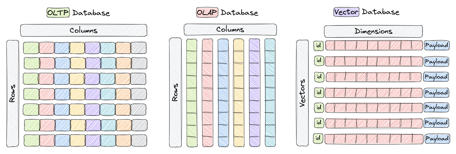
Vector databases are a type of database designed to store and query high-dimensional vectors
efficiently. In traditional [OLTP](https://www.ibm.com/topics/oltp) and [OLAP](https://www.ibm.com/topics/olap)
databases (as seen in the image above), data is organized in rows and columns (and these are
called **Tables**), and queries are performed based on the values in those columns. However,
in certain applications including image recognition, natural language processing, and recommendation
systems, data is often represented as vectors in a high-dimensional space, and these vectors, plus
an id and a payload, are the elements we store in something called a **Collection** a vector
database like Qdrant.
A vector in this context is a mathematical representation of an object or data point, where each
element of the vector corresponds to a specific feature or attribute of the object. For example,
in an image recognition system, a vector could represent an image, with each element of the vector
representing a pixel value or a descriptor/characteristic of that pixel. In a music recommendation
system, each vector would represent a song, and each element of the vector would represent a
characteristic song such as tempo, genre, lyrics, and so on.
Vector databases are optimized for **storing** and **querying** these high-dimensional vectors
efficiently, and they often using specialized data structures and indexing techniques such as
Hierarchical Navigable Small World (HNSW) -- which is used to implement Approximate Nearest
Neighbors -- and Product Quantization, among others. These databases enable fast similarity
and semantic search while allowing users to find vectors that are the closest to a given query
vector based on some distance metric. The most commonly used distance metrics are Euclidean
Distance, Cosine Similarity, and Dot Product, and these three are fully supported Qdrant.
Here's a quick overview of the three:
- [**Cosine Similarity**](https://en.wikipedia.org/wiki/Cosine_similarity) - Cosine similarity
is a way to measure how similar two things are. Think of it like a ruler that tells you how far
apart two points are, but instead of measuring distance, it measures how similar two things
are. It's often used with text to compare how similar two documents or sentences are to each
other. The output of the cosine similarity ranges from -1 to 1, where -1 means the two things
are completely dissimilar, and 1 means the two things are exactly the same. It's a straightforward
and effective way to compare two things!
- [**Dot Product**](https://en.wikipedia.org/wiki/Dot_product) - The dot product similarity
metric is another way of measuring how similar two things are, like cosine similarity. It's
often used in machine learning and data science when working with numbers. The dot product
similarity is calculated by multiplying the values in two sets of numbers, and then adding
up those products. The higher the sum, the more similar the two sets of numbers are. So, it's
like a scale that tells you how closely two sets of numbers match each other.
- [**Euclidean Distance**](https://en.wikipedia.org/wiki/Euclidean_distance) - Euclidean
distance is a way to measure the distance between two points in space, similar to how we
measure the distance between two places on a map. It's calculated by finding the square root
of the sum of the squared differences between the two points' coordinates. This distance metric
is commonly used in machine learning to measure how similar or dissimilar two data points are
or, in other words, to understand how far apart they are.
Now that we know what vector databases are and how they are structurally different than other
databases, let's go over why they are important.
## Why do we need Vector Databases?
Vector databases play a crucial role in various applications that require similarity search, such
as recommendation systems, content-based image retrieval, and personalized search. By taking
advantage of their efficient indexing and searching techniques, vector databases enable faster
and more accurate retrieval of unstructured data already represented as vectors, which can
help put in front of users the most relevant results to their queries.
In addition, other benefits of using vector databases include:
1. Efficient storage and indexing of high-dimensional data.
3. Ability to handle large-scale datasets with billions of data points.
4. Support for real-time analytics and queries.
5. Ability to handle vectors derived from complex data types such as images, videos, and natural language text.
6. Improved performance and reduced latency in machine learning and AI applications.
7. Reduced development and deployment time and cost compared to building a custom solution.
Keep in mind that the specific benefits of using a vector database may vary depending on the
use case of your organization and the features of the database you ultimately choose.
Let's now evaluate, at a high-level, the way Qdrant is architected.
## High-Level Overview of Qdrant's Architecture
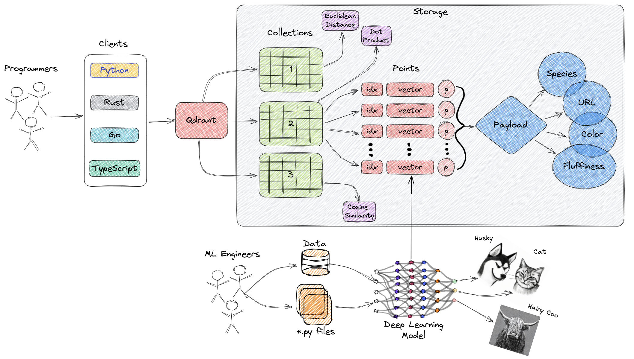
The diagram above represents a high-level overview of some of the main components of Qdrant. Here
are the terminologies you should get familiar with.
- [Collections](../concepts/collections/): A collection is a named set of points (vectors with a payload) among which you can search. The vector of each point within the same collection must have the same dimensionality and be compared by a single metric. [Named vectors](../concepts/collections/#collection-with-multiple-vectors) can be used to have multiple vectors in a single point, each of which can have their own dimensionality and metric requirements.
- [Distance Metrics](https://en.wikipedia.org/wiki/Metric_space): These are used to measure
similarities among vectors and they must be selected at the same time you are creating a
collection. The choice of metric depends on the way the vectors were obtained and, in particular,
on the neural network that will be used to encode new queries.
- [Points](../concepts/points/): The points are the central entity that
Qdrant operates with and they consist of a vector and an optional id and payload.
- id: a unique identifier for your vectors.
- Vector: a high-dimensional representation of data, for example, an image, a sound, a document, a video, etc.
- [Payload](../concepts/payload/): A payload is a JSON object with additional data you can add to a vector.
- [Storage](../concepts/storage/): Qdrant can use one of two options for
storage, **In-memory** storage (Stores all vectors in RAM, has the highest speed since disk
access is required only for persistence), or **Memmap** storage, (creates a virtual address
space associated with the file on disk).
- Clients: the programming languages you can use to connect to Qdrant.
## Next Steps
Now that you know more about vector databases and Qdrant, you are ready to get started with one
of our tutorials. If you've never used a vector database, go ahead and jump straight into
the **Getting Started** section. Conversely, if you are a seasoned developer in these
technology, jump to the section most relevant to your use case.
As you go through the tutorials, please let us know if any questions come up in our
[Discord channel here](https://qdrant.to/discord). 😎
",documentation/overview/_index.md
"---
title: ""Qdrant 1.7.0 has just landed!""
short_description: ""Qdrant 1.7.0 brought a bunch of new features. Let's take a closer look at them!""
description: ""Sparse vectors, Discovery API, user-defined sharding, and snapshot-based shard transfer. That's what you can find in the latest Qdrant 1.7.0 release!""
social_preview_image: /articles_data/qdrant-1.7.x/social_preview.png
small_preview_image: /articles_data/qdrant-1.7.x/icon.svg
preview_dir: /articles_data/qdrant-1.7.x/preview
weight: -90
author: Kacper Łukawski
author_link: https://kacperlukawski.com
date: 2023-12-10T10:00:00Z
draft: false
keywords:
- vector search
- new features
- sparse vectors
- discovery
- exploration
- custom sharding
- snapshot-based shard transfer
- hybrid search
- bm25
- tfidf
- splade
---
Please welcome the long-awaited [Qdrant 1.7.0 release](https://github.com/qdrant/qdrant/releases/tag/v1.7.0). Except for a handful of minor fixes and improvements, this release brings some cool brand-new features that we are excited to share!
The latest version of your favorite vector search engine finally supports **sparse vectors**. That's the feature many of you requested, so why should we ignore it?
We also decided to continue our journey with [vector similarity beyond search](/articles/vector-similarity-beyond-search/). The new Discovery API covers some utterly new use cases. We're more than excited to see what you will build with it!
But there is more to it! Check out what's new in **Qdrant 1.7.0**!
1. Sparse vectors: do you want to use keyword-based search? Support for sparse vectors is finally here!
2. Discovery API: an entirely new way of using vectors for restricted search and exploration.
3. User-defined sharding: you can now decide which points should be stored on which shard.
4. Snapshot-based shard transfer: a new option for moving shards between nodes.
Do you see something missing? Your feedback drives the development of Qdrant, so do not hesitate to [join our Discord community](https://qdrant.to/discord) and help us build the best vector search engine out there!
## New features
Qdrant 1.7.0 brings a bunch of new features. Let's take a closer look at them!
### Sparse vectors
Traditional keyword-based search mechanisms often rely on algorithms like TF-IDF, BM25, or comparable methods. While these techniques internally utilize vectors, they typically involve sparse vector representations. In these methods, the **vectors are predominantly filled with zeros, containing a relatively small number of non-zero values**.
Those sparse vectors are theoretically high dimensional, definitely way higher than the dense vectors used in semantic search. However, since the majority of dimensions are usually zeros, we store them differently and just keep the non-zero dimensions.
Until now, Qdrant has not been able to handle sparse vectors natively. Some were trying to convert them to dense vectors, but that was not the best solution or a suggested way. We even wrote a piece with [our thoughts on building a hybrid search](/articles/hybrid-search/), and we encouraged you to use a different tool for keyword lookup.
Things have changed since then, as so many of you wanted a single tool for sparse and dense vectors. And responding to this [popular](https://github.com/qdrant/qdrant/issues/1678) [demand](https://github.com/qdrant/qdrant/issues/1135), we've now introduced sparse vectors!
If you're coming across the topic of sparse vectors for the first time, our [Brief History of Search](https://qdrant.tech/documentation/overview/vector-search/) explains the difference between sparse and dense vectors.
Check out the [sparse vectors article](../sparse-vectors/) and [sparse vectors index docs](/documentation/concepts/indexing/#sparse-vector-index) for more details on what this new index means for Qdrant users.
### Discovery API
The recently launched [Discovery API](/documentation/concepts/explore/#discovery-api) extends the range of scenarios for leveraging vectors. While its interface mirrors the [Recommendation API](/documentation/concepts/explore/#recommendation-api), it focuses on refining the search parameters for greater precision.
The concept of 'context' refers to a collection of positive-negative pairs that define zones within a space. Each pair effectively divides the space into positive or negative segments. This concept guides the search operation to prioritize points based on their inclusion within positive zones or their avoidance of negative zones. Essentially, the search algorithm favors points that fall within multiple positive zones or steer clear of negative ones.
The Discovery API can be used in two ways - either with or without the target point. The first case is called a **discovery search**, while the second is called a **context search**.
#### Discovery search
*Discovery search* is an operation that uses a target point to find the most relevant points in the collection, while performing the search in the preferred areas only. That is basically a search operation with more control over the search space.

Please refer to the [Discovery API documentation on discovery search](/documentation/concepts/explore/#discovery-search) for more details and the internal mechanics of the operation.
#### Context search
The mode of *context search* is similar to the discovery search, but it does not use a target point. Instead, the `context` is used to navigate the [HNSW graph](https://arxiv.org/abs/1603.09320) towards preferred zones. It is expected that the results in that mode will be diverse, and not centered around one point.
*Context Search* could serve as a solution for individuals seeking a more exploratory approach to navigate the vector space.

### User-defined sharding
Qdrant's collections are divided into shards. A single **shard** is a self-contained store of points, which can be moved between nodes. Up till now, the points were distributed among shards by using a consistent hashing algorithm, so that shards were managing non-intersecting subsets of points.
The latter one remains true, but now you can define your own sharding and decide which points should be stored on which shard. Sounds cool, right? But why would you need that? Well, there are multiple scenarios in which you may want to use custom sharding. For example, you may want to store some points on a dedicated node, or you may want to store points from the same user on the same shard and
While the existing behavior is still the default one, you can now define the shards when you create a collection. Then, you can assign each point to a shard by providing a `shard_key` in the `upsert` operation. What's more, you can also search over the selected shards only, by providing the `shard_key` parameter in the search operation.
```http request
POST /collections/my_collection/points/search
{
""vector"": [0.29, 0.81, 0.75, 0.11],
""shard_key"": [""cats"", ""dogs""],
""limit"": 10,
""with_payload"": true,
}
```
If you want to know more about the user-defined sharding, please refer to the [sharding documentation](/documentation/guides/distributed_deployment/#sharding).
### Snapshot-based shard transfer
That's a really more in depth technical improvement for the distributed mode users, that we implemented a new options the shard transfer mechanism. The new approach is based on the snapshot of the shard, which is transferred to the target node.
Moving shards is required for dynamical scaling of the cluster. Your data can migrate between nodes, and the way you move it is crucial for the performance of the whole system. The good old `stream_records` method (still the default one) transmits all the records between the machines and indexes them on the target node.
In the case of moving the shard, it's necessary to recreate the HNSW index each time. However, with the introduction of the new `snapshot` approach, the snapshot itself, inclusive of all data and potentially quantized content, is transferred to the target node. This comprehensive snapshot includes the entire index, enabling the target node to seamlessly load it and promptly begin handling requests without the need for index recreation.
There are multiple scenarios in which you may prefer one over the other. Please check out the docs of the [shard transfer method](/documentation/guides/distributed_deployment/#shard-transfer-method) for more details and head-to-head comparison. As for now, the old `stream_records` method is still the default one, but we may decide to change it in the future.
## Minor improvements
Beyond introducing new features, Qdrant 1.7.0 enhances performance and addresses various minor issues. Here's a rundown of the key improvements:
1. Improvement of HNSW Index Building on High CPU Systems ([PR#2869](https://github.com/qdrant/qdrant/pull/2869)).
2. Improving [Search Tail Latencies](https://github.com/qdrant/qdrant/pull/2931): improvement for high CPU systems with many parallel searches, directly impacting the user experience by reducing latency.
3. [Adding Index for Geo Map Payloads](https://github.com/qdrant/qdrant/pull/2768): index for geo map payloads can significantly improve search performance, especially for applications involving geographical data.
4. Stability of Consensus on Big High Load Clusters: enhancing the stability of consensus in large, high-load environments is critical for ensuring the reliability and scalability of the system ([PR#3013](https://github.com/qdrant/qdrant/pull/3013), [PR#3026](https://github.com/qdrant/qdrant/pull/3026), [PR#2942](https://github.com/qdrant/qdrant/pull/2942), [PR#3103](https://github.com/qdrant/qdrant/pull/3103), [PR#3054](https://github.com/qdrant/qdrant/pull/3054)).
5. Configurable Timeout for Searches: allowing users to configure the timeout for searches provides greater flexibility and can help optimize system performance under different operational conditions ([PR#2748](https://github.com/qdrant/qdrant/pull/2748), [PR#2771](https://github.com/qdrant/qdrant/pull/2771)).
## Release notes
[Our release notes](https://github.com/qdrant/qdrant/releases/tag/v1.7.0) are a place to go if you are interested in more details. Please remember that Qdrant is an open source project, so feel free to [contribute](https://github.com/qdrant/qdrant/issues)!
",articles/qdrant-1.7.x.md
"---
title: Metric Learning Tips & Tricks
short_description: How to train an object matching model and serve it in production.
description: Practical recommendations on how to train a matching model and serve it in production. Even with no labeled data.
# external_link: https://vasnetsov93.medium.com/metric-learning-tips-n-tricks-2e4cfee6b75b
social_preview_image: /articles_data/metric-learning-tips/preview/social_preview.jpg
preview_dir: /articles_data/metric-learning-tips/preview
small_preview_image: /articles_data/metric-learning-tips/scatter-graph.svg
weight: 20
author: Andrei Vasnetsov
author_link: https://blog.vasnetsov.com/
date: 2021-05-15T10:18:00.000Z
# aliases: [ /articles/metric-learning-tips/ ]
---
## How to train object matching model with no labeled data and use it in production
Currently, most machine-learning-related business cases are solved as a classification problems.
Classification algorithms are so well studied in practice that even if the original problem is not directly a classification task, it is usually decomposed or approximately converted into one.
However, despite its simplicity, the classification task has requirements that could complicate its production integration and scaling.
E.g. it requires a fixed number of classes, where each class should have a sufficient number of training samples.
In this article, I will describe how we overcome these limitations by switching to metric learning.
By the example of matching job positions and candidates, I will show how to train metric learning model with no manually labeled data, how to estimate prediction confidence, and how to serve metric learning in production.
## What is metric learning and why using it?
According to Wikipedia, metric learning is the task of learning a distance function over objects.
In practice, it means that we can train a model that tells a number for any pair of given objects.
And this number should represent a degree or score of similarity between those given objects.
For example, objects with a score of 0.9 could be more similar than objects with a score of 0.5
Actual scores and their direction could vary among different implementations.
In practice, there are two main approaches to metric learning and two corresponding types of NN architectures.
The first is the interaction-based approach, which first builds local interactions (i.e., local matching signals) between two objects. Deep neural networks learn hierarchical interaction patterns for matching.
Examples of neural network architectures include MV-LSTM, ARC-II, and MatchPyramid.

> MV-LSTM, example of interaction-based model, [Shengxian Wan et al.
](https://www.researchgate.net/figure/Illustration-of-MV-LSTM-S-X-and-S-Y-are-the-in_fig1_285271115) via Researchgate
The second is the representation-based approach.
In this case distance function is composed of 2 components:
the Encoder transforms an object into embedded representation - usually a large float point vector, and the Comparator takes embeddings of a pair of objects from the Encoder and calculates their similarity.
The most well-known example of this embedding representation is Word2Vec.
Examples of neural network architectures also include DSSM, C-DSSM, and ARC-I.
The Comparator is usually a very simple function that could be calculated very quickly.
It might be cosine similarity or even a dot production.
Two-stage schema allows performing complex calculations only once per object.
Once transformed, the Comparator can calculate object similarity independent of the Encoder much more quickly.
For more convenience, embeddings can be placed into specialized storages or vector search engines.
These search engines allow to manage embeddings using API, perform searches and other operations with vectors.

> C-DSSM, example of representation-based model, [Xue Li et al.](https://arxiv.org/abs/1901.10710v2) via arXiv
Pre-trained NNs can also be used. The output of the second-to-last layer could work as an embedded representation.
Further in this article, I would focus on the representation-based approach, as it proved to be more flexible and fast.
So what are the advantages of using metric learning comparing to classification?
Object Encoder does not assume the number of classes.
So if you can't split your object into classes,
if the number of classes is too high, or you suspect that it could grow in the future - consider using metric learning.
In our case, business goal was to find suitable vacancies for candidates who specify the title of the desired position.
To solve this, we used to apply a classifier to determine the job category of the vacancy and the candidate.
But this solution was limited to only a few hundred categories.
Candidates were complaining that they couldn't find the right category for them.
Training the classifier for new categories would be too long and require new training data for each new category.
Switching to metric learning allowed us to overcome these limitations, the resulting solution could compare any pair position descriptions, even if we don't have this category reference yet.

> T-SNE with job samples, Image by Author. Play with [Embedding Projector](https://projector.tensorflow.org/?config=https://gist.githubusercontent.com/generall/7e712425e3b340c2c4dbc1a29f515d91/raw/b45b2b6f6c1d5ab3d3363c50805f3834a85c8879/config.json) yourself.
With metric learning, we learn not a concrete job type but how to match job descriptions from a candidate's CV and a vacancy.
Secondly, with metric learning, it is easy to add more reference occupations without model retraining.
We can then add the reference to a vector search engine.
Next time we will match occupations - this new reference vector will be searchable.
## Data for metric learning
Unlike classifiers, a metric learning training does not require specific class labels.
All that is required are examples of similar and dissimilar objects.
We would call them positive and negative samples.
At the same time, it could be a relative similarity between a pair of objects.
For example, twins look more alike to each other than a pair of random people.
And random people are more similar to each other than a man and a cat.
A model can use such relative examples for learning.
The good news is that the division into classes is only a special case of determining similarity.
To use such datasets, it is enough to declare samples from one class as positive and samples from another class as negative.
In this way, it is possible to combine several datasets with mismatched classes into one generalized dataset for metric learning.
But not only datasets with division into classes are suitable for extracting positive and negative examples.
If, for example, there are additional features in the description of the object, the value of these features can also be used as a similarity factor.
It may not be as explicit as class membership, but the relative similarity is also suitable for learning.
In the case of job descriptions, there are many ontologies of occupations, which were able to be combined into a single dataset thanks to this approach.
We even went a step further and used identical job titles to find similar descriptions.
As a result, we got a self-supervised universal dataset that did not require any manual labeling.
Unfortunately, universality does not allow some techniques to be applied in training.
Next, I will describe how to overcome this disadvantage.
## Training the model
There are several ways to train a metric learning model.
Among the most popular is the use of Triplet or Contrastive loss functions, but I will not go deep into them in this article.
However, I will tell you about one interesting trick that helped us work with unified training examples.
One of the most important practices to efficiently train the metric learning model is hard negative mining.
This technique aims to include negative samples on which model gave worse predictions during the last training epoch.
Most articles that describe this technique assume that training data consists of many small classes (in most cases it is people's faces).
With data like this, it is easy to find bad samples - if two samples from different classes have a high similarity score, we can use it as a negative sample.
But we had no such classes in our data, the only thing we have is occupation pairs assumed to be similar in some way.
We cannot guarantee that there is no better match for each job occupation among this pair.
That is why we can't use hard negative mining for our model.

> [Alfonso Medela et al.](https://arxiv.org/abs/1905.10675) via arXiv
To compensate for this limitation we can try to increase the number of random (weak) negative samples.
One way to achieve this is to train the model longer, so it will see more samples by the end of the training.
But we found a better solution in adjusting our loss function.
In a regular implementation of Triplet or Contractive loss, each positive pair is compared with some or a few negative samples.
What we did is we allow pair comparison amongst the whole batch.
That means that loss-function penalizes all pairs of random objects if its score exceeds any of the positive scores in a batch.
This extension gives `~ N * B^2` comparisons where `B` is a size of batch and `N` is a number of batches.
Much bigger than `~ N * B` in regular triplet loss.
This means that increasing the size of the batch significantly increases the number of negative comparisons, and therefore should improve the model performance.
We were able to observe this dependence in our experiments.
Similar idea we also found in the article [Supervised Contrastive Learning](https://arxiv.org/abs/2004.11362).
## Model confidence
In real life it is often needed to know how confident the model was in the prediction.
Whether manual adjustment or validation of the result is required.
With conventional classification, it is easy to understand by scores how confident the model is in the result.
If the probability values of different classes are close to each other, the model is not confident.
If, on the contrary, the most probable class differs greatly, then the model is confident.
At first glance, this cannot be applied to metric learning.
Even if the predicted object similarity score is small it might only mean that the reference set has no proper objects to compare with.
Conversely, the model can group garbage objects with a large score.
Fortunately, we found a small modification to the embedding generator, which allows us to define confidence in the same way as it is done in conventional classifiers with a Softmax activation function.
The modification consists in building an embedding as a combination of feature groups.
Each feature group is presented as a one-hot encoded sub-vector in the embedding.
If the model can confidently predict the feature value - the corresponding sub-vector will have a high absolute value in some of its elements.
For a more intuitive understanding, I recommend thinking about embeddings not as points in space, but as a set of binary features.
To implement this modification and form proper feature groups we would need to change a regular linear output layer to a concatenation of several Softmax layers.
Each softmax component would represent an independent feature and force the neural network to learn them.
Let's take for example that we have 4 softmax components with 128 elements each.
Every such component could be roughly imagined as a one-hot-encoded number in the range of 0 to 127.
Thus, the resulting vector will represent one of `128^4` possible combinations.
If the trained model is good enough, you can even try to interpret the values of singular features individually.

> Softmax feature embeddings, Image by Author.
## Neural rules
Machine learning models rarely train to 100% accuracy.
In a conventional classifier, errors can only be eliminated by modifying and repeating the training process.
Metric training, however, is more flexible in this matter and allows you to introduce additional steps that allow you to correct the errors of an already trained model.
A common error of the metric learning model is erroneously declaring objects close although in reality they are not.
To correct this kind of error, we introduce exclusion rules.
Rules consist of 2 object anchors encoded into vector space.
If the target object falls into one of the anchors' effects area - it triggers the rule. It will exclude all objects in the second anchor area from the prediction result.

> Neural exclusion rules, Image by Author.
The convenience of working with embeddings is that regardless of the number of rules,
you only need to perform the encoding once per object.
Then to find a suitable rule, it is enough to compare the target object's embedding and the pre-calculated embeddings of the rule's anchors.
Which, when implemented, translates into just one additional query to the vector search engine.
## Vector search in production
When implementing a metric learning model in production, the question arises about the storage and management of vectors.
It should be easy to add new vectors if new job descriptions appear in the service.
In our case, we also needed to apply additional conditions to the search.
We needed to filter, for example, the location of candidates and the level of language proficiency.
We did not find a ready-made tool for such vector management, so we created [Qdrant](https://github.com/qdrant/qdrant) - open-source vector search engine.
It allows you to add and delete vectors with a simple API, independent of a programming language you are using.
You can also assign the payload to vectors.
This payload allows additional filtering during the search request.
Qdrant has a pre-built docker image and start working with it is just as simple as running
```bash
docker run -p 6333:6333 qdrant/qdrant
```
Documentation with examples could be found [here](https://qdrant.github.io/qdrant/redoc/index.html).
## Conclusion
In this article, I have shown how metric learning can be more scalable and flexible than the classification models.
I suggest trying similar approaches in your tasks - it might be matching similar texts, images, or audio data.
With the existing variety of pre-trained neural networks and a vector search engine, it is easy to build your metric learning-based application.
",articles/metric-learning-tips.md
"---
title: Qdrant 0.10 released
short_description: A short review of all the features introduced in Qdrant 0.10
description: Qdrant 0.10 brings a lot of changes. Check out what's new!
preview_dir: /articles_data/qdrant-0-10-release/preview
small_preview_image: /articles_data/qdrant-0-10-release/new-svgrepo-com.svg
social_preview_image: /articles_data/qdrant-0-10-release/preview/social_preview.jpg
weight: 70
author: Kacper Łukawski
author_link: https://medium.com/@lukawskikacper
date: 2022-09-19T13:30:00+02:00
draft: false
---
[Qdrant 0.10 is a new version](https://github.com/qdrant/qdrant/releases/tag/v0.10.0) that brings a lot of performance
improvements, but also some new features which were heavily requested by our users. Here is an overview of what has changed.
## Storing multiple vectors per object
Previously, if you wanted to use semantic search with multiple vectors per object, you had to create separate collections
for each vector type. This was even if the vectors shared some other attributes in the payload. With Qdrant 0.10, you can
now store all of these vectors together in the same collection, which allows you to share a single copy of the payload.
This makes it easier to use semantic search with multiple vector types, and reduces the amount of work you need to do to
set up your collections.
## Batch vector search
Previously, you had to send multiple requests to the Qdrant API to perform multiple non-related tasks. However, this
can cause significant network overhead and slow down the process, especially if you have a poor connection speed.
Fortunately, the [new batch search feature](https://blog.qdrant.tech/batch-vector-search-with-qdrant-8c4d598179d5) allows
you to avoid this issue. With just one API call, Qdrant will handle multiple search requests in the most efficient way
possible. This means that you can perform multiple tasks simultaneously without having to worry about network overhead
or slow performance.
## Built-in ARM support
To make our application accessible to ARM users, we have compiled it specifically for that platform. If it is not
compiled for ARM, the device will have to emulate it, which can slow down performance. To ensure the best possible
experience for ARM users, we have created Docker images specifically for that platform. Keep in mind that using
a limited set of processor instructions may affect the performance of your vector search. Therefore, [we have tested
both ARM and non-ARM architectures using similar setups to understand the potential impact on performance
](https://blog.qdrant.tech/qdrant-supports-arm-architecture-363e92aa5026).
## Full-text filtering
Qdrant is a vector database that allows you to quickly search for the nearest neighbors. However, you may need to apply
additional filters on top of the semantic search. Up until version 0.10, Qdrant only supported keyword filters. With the
release of Qdrant 0.10, [you can now use full-text filters](https://blog.qdrant.tech/qdrant-introduces-full-text-filters-and-indexes-9a032fcb5fa)
as well. This new filter type can be used on its own or in combination with other filter types to provide even more
flexibility in your searches.
",articles/qdrant-0-10-release.md
"---
title: ""Question Answering with LangChain and Qdrant without boilerplate""
short_description: ""Large Language Models might be developed fast with modern tool. Here is how!""
description: ""We combined LangChain, pretrained LLM from OpenAI, SentenceTransformers and Qdrant to create a Q&A system with just a few lines of code.""
social_preview_image: /articles_data/langchain-integration/social_preview.png
small_preview_image: /articles_data/langchain-integration/chain.svg
preview_dir: /articles_data/langchain-integration/preview
weight: 6
author: Kacper Łukawski
author_link: https://medium.com/@lukawskikacper
date: 2023-01-31T10:53:20+01:00
draft: false
keywords:
- vector search
- langchain
- llm
- large language models
- question answering
- openai
- embeddings
---
Building applications with Large Language Models don't have to be complicated. A lot has been going on recently to simplify the development,
so you can utilize already pre-trained models and support even complex pipelines with a few lines of code. [LangChain](https://langchain.readthedocs.io)
provides unified interfaces to different libraries, so you can avoid writing boilerplate code and focus on the value you want to bring.
## Question Answering with Qdrant in the loop
It has been reported millions of times recently, but let's say that again. ChatGPT-like models struggle with generating factual statements if no context
is provided. They have some general knowledge but cannot guarantee to produce a valid answer consistently. Thus, it is better to provide some facts we
know are actual, so it can just choose the valid parts and extract them from all the provided contextual data to give a comprehensive answer. Vector database,
such as Qdrant, is of great help here, as their ability to perform a semantic search over a huge knowledge base is crucial to preselect some possibly valid
documents, so they can be provided into the LLM. That's also one of the **chains** implemented in LangChain, which is called `VectorDBQA`. And Qdrant got
integrated with the library, so it might be used to build it effortlessly.
### What do we need?
Surprisingly enough, there will be two models required to set things up. First of all, we need an embedding model that will convert the set of facts into
vectors, and store those into Qdrant. That's an identical process to any other semantic search application. We're going to use one of the
`SentenceTransformers` models, so it can be hosted locally. The embeddings created by that model will be put into Qdrant and used to retrieve the most
similar documents, given the query.
However, when we receive a query, there are two steps involved. First of all, we ask Qdrant to provide the most relevant documents and simply combine all
of them into a single text. Then, we build a prompt to the LLM (in our case OpenAI), including those documents as a context, of course together with the
question asked. So the input to the LLM looks like the following:
```text
Use the following pieces of context to answer the question at the end. If you don't know the answer, just say that you don't know, don't try to make up an answer.
It's as certain as 2 + 2 = 4
...
Question: How much is 2 + 2?
Helpful Answer:
```
There might be several context documents combined, and it is solely up to LLM to choose the right piece of content. But our expectation is, the model should
respond with just `4`.
Why do we need two different models? Both solve some different tasks. The first model performs feature extraction, by converting the text into vectors, while
the second one helps in text generation or summarization. Disclaimer: This is not the only way to solve that task with LangChain. Such a chain is called `stuff`
in the library nomenclature.

Enough theory! This sounds like a pretty complex application, as it involves several systems. But with LangChain, it might be implemented in just a few lines
of code, thanks to the recent integration with Qdrant. We're not even going to work directly with `QdrantClient`, as everything is already done in the background
by LangChain. If you want to get into the source code right away, all the processing is available as a
[Google Colab notebook](https://colab.research.google.com/drive/19RxxkZdnq_YqBH5kBV10Rt0Rax-kminD?usp=sharing).
## Implementing Question Answering with LangChain and Qdrant
### Configuration
A journey of a thousand miles begins with a single step, in our case with the configuration of all the services. We'll be using [Qdrant Cloud](https://qdrant.tech),
so we need an API key. The same is for OpenAI - the API key has to be obtained from their website.

### Building the knowledge base
We also need some facts from which the answers will be generated. There is plenty of public datasets available, and
[Natural Questions](https://ai.google.com/research/NaturalQuestions/visualization) is one of them. It consists of the whole HTML content of the websites they were
scraped from. That means we need some preprocessing to extract plain text content. As a result, we’re going to have two lists of strings - one for questions and
the other one for the answers.
The answers have to be vectorized with the first of our models. The `sentence-transformers/all-mpnet-base-v2` is one of the possibilities, but there are some
other options available. LangChain will handle that part of the process in a single function call.

### Setting up QA with Qdrant in a loop
`VectorDBQA` is a chain that performs the process described above. So it, first of all, loads some facts from Qdrant and then feeds them into OpenAI LLM which
should analyze them to find the answer to a given question. The only last thing to do before using it is to put things together, also with a single function call.

## Testing out the chain
And that's it! We can put some queries, and LangChain will perform all the required processing to find the answer in the provided context.

```text
> what kind of music is scott joplin most famous for
Scott Joplin is most famous for composing ragtime music.
> who died from the band faith no more
Chuck Mosley
> when does maggie come on grey's anatomy
Maggie first appears in season 10, episode 1, which aired on September 26, 2013.
> can't take my eyes off you lyrics meaning
I don't know.
> who lasted the longest on alone season 2
David McIntyre lasted the longest on Alone season 2, with a total of 66 days.
```
The great thing about such a setup is that the knowledge base might be easily extended with some new facts and those will be included in the prompts
sent to LLM later on. Of course, assuming their similarity to the given question will be in the top results returned by Qdrant.
If you want to run the chain on your own, the simplest way to reproduce it is to open the
[Google Colab notebook](https://colab.research.google.com/drive/19RxxkZdnq_YqBH5kBV10Rt0Rax-kminD?usp=sharing).
",articles/langchain-integration.md
"---
title: ""Enhance OpenAI Embeddings with Qdrant's Binary Quantization""
draft: false
slug: binary-quantization-openai
short_description: Use Qdrant's Binary Quantization to enhance OpenAI embeddings
description: Use Qdrant's Binary Quantization to enhance the performance and efficiency of OpenAI embeddings
preview_dir: /articles_data/binary-quantization-openai/preview
preview_image: /articles-data/binary-quantization-openai/Article-Image.png # Change this
small_preview_image: /articles_data/binary-quantization-openai/icon.svg
social_preview_image: /articles_data/binary-quantization-openai/preview/social-preview.png
title_preview_image: /articles_data/binary-quantization-openai/preview/preview.webp # Optional image used for blog post title
date: 2024-02-21T13:12:08-08:00
author: Nirant Kasliwal
author_link: https://www.linkedin.com/in/nirant/
featured: false
tags:
- OpenAI
- binary quantization
- embeddings
weight: -130
aliases: [ /blog/binary-quantization-openai/ ]
---
OpenAI Ada-003 embeddings are a powerful tool for natural language processing (NLP). However, the size of the embeddings are a challenge, especially with real-time search and retrieval. In this article, we explore how you can use Qdrant's Binary Quantization to enhance the performance and efficiency of OpenAI embeddings.
In this post, we discuss:
- The significance of OpenAI embeddings and real-world challenges.
- Qdrant's Binary Quantization, and how it can improve the performance of OpenAI embeddings
- Results of an experiment that highlights improvements in search efficiency and accuracy
- Implications of these findings for real-world applications
- Best practices for leveraging Binary Quantization to enhance OpenAI embeddings
You can also try out these techniques as described in [Binary Quantization OpenAI](https://github.com/qdrant/examples/blob/openai-3/binary-quantization-openai/README.md), which includes Jupyter notebooks.
## New OpenAI Embeddings: Performance and Changes
As the technology of embedding models has advanced, demand has grown. Users are looking more for powerful and efficient text-embedding models. OpenAI's Ada-003 embeddings offer state-of-the-art performance on a wide range of NLP tasks, including those noted in [MTEB](https://huggingface.co/spaces/mteb/leaderboard) and [MIRACL](https://openai.com/blog/new-embedding-models-and-api-updates).
These models include multilingual support in over 100 languages. The transition from text-embedding-ada-002 to text-embedding-3-large has led to a significant jump in performance scores (from 31.4% to 54.9% on MIRACL).
#### Matryoshka Representation Learning
The new OpenAI models have been trained with a novel approach called ""[Matryoshka Representation Learning](https://aniketrege.github.io/blog/2024/mrl/)"". Developers can set up embeddings of different sizes (number of dimensions). In this post, we use small and large variants. Developers can select embeddings which balances accuracy and size.
Here, we show how the accuracy of binary quantization is quite good across different dimensions -- for both the models.
## Enhanced Performance and Efficiency with Binary Quantization
By reducing storage needs, you can scale applications with lower costs. This addresses a critical challenge posed by the original embedding sizes. Binary Quantization also speeds the search process. It simplifies the complex distance calculations between vectors into more manageable bitwise operations, which supports potentially real-time searches across vast datasets.
The accompanying graph illustrates the promising accuracy levels achievable with binary quantization across different model sizes, showcasing its practicality without severely compromising on performance. This dual advantage of storage reduction and accelerated search capabilities underscores the transformative potential of Binary Quantization in deploying OpenAI embeddings more effectively across various real-world applications.

The efficiency gains from Binary Quantization are as follows:
- Reduced storage footprint: It helps with large-scale datasets. It also saves on memory, and scales up to 30x at the same cost.
- Enhanced speed of data retrieval: Smaller data sizes generally leads to faster searches.
- Accelerated search process: It is based on simplified distance calculations between vectors to bitwise operations. This enables real-time querying even in extensive databases.
### Experiment Setup: OpenAI Embeddings in Focus
To identify Binary Quantization's impact on search efficiency and accuracy, we designed our experiment on OpenAI text-embedding models. These models, which capture nuanced linguistic features and semantic relationships, are the backbone of our analysis. We then delve deep into the potential enhancements offered by Qdrant's Binary Quantization feature.
This approach not only leverages the high-caliber OpenAI embeddings but also provides a broad basis for evaluating the search mechanism under scrutiny.
#### Dataset
The research employs 100K random samples from the [OpenAI 1M](https://huggingface.co/datasets/KShivendu/dbpedia-entities-openai-1M) 1M dataset, focusing on 100 randomly selected records. These records serve as queries in the experiment, aiming to assess how Binary Quantization influences search efficiency and precision within the dataset. We then use the embeddings of the queries to search for the nearest neighbors in the dataset.
#### Parameters: Oversampling, Rescoring, and Search Limits
For each record, we run a parameter sweep over the number of oversampling, rescoring, and search limits. We can then understand the impact of these parameters on search accuracy and efficiency. Our experiment was designed to assess the impact of Binary Quantization under various conditions, based on the following parameters:
- **Oversampling**: By oversampling, we can limit the loss of information inherent in quantization. This also helps to preserve the semantic richness of your OpenAI embeddings. We experimented with different oversampling factors, and identified the impact on the accuracy and efficiency of search. Spoiler: higher oversampling factors tend to improve the accuracy of searches. However, they usually require more computational resources.
- **Rescoring**: Rescoring refines the first results of an initial binary search. This process leverages the original high-dimensional vectors to refine the search results, **always** improving accuracy. We toggled rescoring on and off to measure effectiveness, when combined with Binary Quantization. We also measured the impact on search performance.
- **Search Limits**: We specify the number of results from the search process. We experimented with various search limits to measure their impact the accuracy and efficiency. We explored the trade-offs between search depth and performance. The results provide insight for applications with different precision and speed requirements.
Through this detailed setup, our experiment sought to shed light on the nuanced interplay between Binary Quantization and the high-quality embeddings produced by OpenAI's models. By meticulously adjusting and observing the outcomes under different conditions, we aimed to uncover actionable insights that could empower users to harness the full potential of Qdrant in combination with OpenAI's embeddings, regardless of their specific application needs.
### Results: Binary Quantization's Impact on OpenAI Embeddings
To analyze the impact of rescoring (`True` or `False`), we compared results across different model configurations and search limits. Rescoring sets up a more precise search, based on results from an initial query.
#### Rescoring

Here are some key observations, which analyzes the impact of rescoring (`True` or `False`):
1. **Significantly Improved Accuracy**:
- Across all models and dimension configurations, enabling rescoring (`True`) consistently results in higher accuracy scores compared to when rescoring is disabled (`False`).
- The improvement in accuracy is true across various search limits (10, 20, 50, 100).
2. **Model and Dimension Specific Observations**:
- For the `text-embedding-3-large` model with 3072 dimensions, rescoring boosts the accuracy from an average of about 76-77% without rescoring to 97-99% with rescoring, depending on the search limit and oversampling rate.
- The accuracy improvement with increased oversampling is more pronounced when rescoring is enabled, indicating a better utilization of the additional binary codes in refining search results.
- With the `text-embedding-3-small` model at 512 dimensions, accuracy increases from around 53-55% without rescoring to 71-91% with rescoring, highlighting the significant impact of rescoring, especially at lower dimensions.
- For higher dimension models (such as text-embedding-3-large with 3072 dimensions),
In contrast, for lower dimension models (such as text-embedding-3-small with 512 dimensions), the incremental accuracy gains from increased oversampling levels are less significant, even with rescoring enabled. This suggests a diminishing return on accuracy improvement with higher oversampling in lower dimension spaces.
3. **Influence of Search Limit**:
- The performance gain from rescoring seems to be relatively stable across different search limits, suggesting that rescoring consistently enhances accuracy regardless of the number of top results considered.
In summary, enabling rescoring dramatically improves search accuracy across all tested configurations. It is crucial feature for applications where precision is paramount. The consistent performance boost provided by rescoring underscores its value in refining search results, particularly when working with complex, high-dimensional data like OpenAI embeddings. This enhancement is critical for applications that demand high accuracy, such as semantic search, content discovery, and recommendation systems, where the quality of search results directly impacts user experience and satisfaction.
### Dataset Combinations
For those exploring the integration of text embedding models with Qdrant, it's crucial to consider various model configurations for optimal performance. The dataset combinations defined above illustrate different configurations to test against Qdrant. These combinations vary by two primary attributes:
1. **Model Name**: Signifying the specific text embedding model variant, such as ""text-embedding-3-large"" or ""text-embedding-3-small"". This distinction correlates with the model's capacity, with ""large"" models offering more detailed embeddings at the cost of increased computational resources.
2. **Dimensions**: This refers to the size of the vector embeddings produced by the model. Options range from 512 to 3072 dimensions. Higher dimensions could lead to more precise embeddings but might also increase the search time and memory usage in Qdrant.
Optimizing these parameters is a balancing act between search accuracy and resource efficiency. Testing across these combinations allows users to identify the configuration that best meets their specific needs, considering the trade-offs between computational resources and the quality of search results.
```python
dataset_combinations = [
{
""model_name"": ""text-embedding-3-large"",
""dimensions"": 3072,
},
{
""model_name"": ""text-embedding-3-large"",
""dimensions"": 1024,
},
{
""model_name"": ""text-embedding-3-large"",
""dimensions"": 1536,
},
{
""model_name"": ""text-embedding-3-small"",
""dimensions"": 512,
},
{
""model_name"": ""text-embedding-3-small"",
""dimensions"": 1024,
},
{
""model_name"": ""text-embedding-3-small"",
""dimensions"": 1536,
},
]
```
#### Exploring Dataset Combinations and Their Impacts on Model Performance
The code snippet iterates through predefined dataset and model combinations. For each combination, characterized by the model name and its dimensions, the corresponding experiment's results are loaded. These results, which are stored in JSON format, include performance metrics like accuracy under different configurations: with and without oversampling, and with and without a rescore step.
Following the extraction of these metrics, the code computes the average accuracy across different settings, excluding extreme cases of very low limits (specifically, limits of 1 and 5). This computation groups the results by oversampling, rescore presence, and limit, before calculating the mean accuracy for each subgroup.
After gathering and processing this data, the average accuracies are organized into a pivot table. This table is indexed by the limit (the number of top results considered), and columns are formed based on combinations of oversampling and rescoring.
```python
import pandas as pd
for combination in dataset_combinations:
model_name = combination[""model_name""]
dimensions = combination[""dimensions""]
print(f""Model: {model_name}, dimensions: {dimensions}"")
results = pd.read_json(f""../results/results-{model_name}-{dimensions}.json"", lines=True)
average_accuracy = results[results[""limit""] != 1]
average_accuracy = average_accuracy[average_accuracy[""limit""] != 5]
average_accuracy = average_accuracy.groupby([""oversampling"", ""rescore"", ""limit""])[
""accuracy""
].mean()
average_accuracy = average_accuracy.reset_index()
acc = average_accuracy.pivot(
index=""limit"", columns=[""oversampling"", ""rescore""], values=""accuracy""
)
print(acc)
```
#### Impact of Oversampling
You can use oversampling in machine learning to counteract imbalances in datasets.
It works well when one class significantly outnumbers others. This imbalance
can skew the performance of models, which favors the majority class at the
expense of others. By creating additional samples from the minority classes,
oversampling helps equalize the representation of classes in the training dataset, thus enabling more fair and accurate modeling of real-world scenarios.
The screenshot showcases the effect of oversampling on model performance metrics. While the actual metrics aren't shown, we expect to see improvements in measures such as precision, recall, or F1-score. These improvements illustrate the effectiveness of oversampling in creating a more balanced dataset. It allows the model to learn a better representation of all classes, not just the dominant one.
Without an explicit code snippet or output, we focus on the role of oversampling in model fairness and performance. Through graphical representation, you can set up before-and-after comparisons. These comparisons illustrate the contribution to machine learning projects.

### Leveraging Binary Quantization: Best Practices
We recommend the following best practices for leveraging Binary Quantization to enhance OpenAI embeddings:
1. Embedding Model: Use the text-embedding-3-large from MTEB. It is most accurate among those tested.
2. Dimensions: Use the highest dimension available for the model, to maximize accuracy. The results are true for English and other languages.
3. Oversampling: Use an oversampling factor of 3 for the best balance between accuracy and efficiency. This factor is suitable for a wide range of applications.
4. Rescoring: Enable rescoring to improve the accuracy of search results.
5. RAM: Store the full vectors and payload on disk. Limit what you load from memory to the binary quantization index. This helps reduce the memory footprint and improve the overall efficiency of the system. The incremental latency from the disk read is negligible compared to the latency savings from the binary scoring in Qdrant, which uses SIMD instructions where possible.
Want to discuss these findings and learn more about Binary Quantization? [Join our Discord community.](https://discord.gg/qdrant)
Learn more about how to boost your vector search speed and accuracy while reducing costs: [Binary Quantization.](https://qdrant.tech/documentation/guides/quantization/?selector=aHRtbCA%2BIGJvZHkgPiBkaXY6bnRoLW9mLXR5cGUoMSkgPiBzZWN0aW9uID4gZGl2ID4gZGl2ID4gZGl2Om50aC1vZi10eXBlKDIpID4gYXJ0aWNsZSA%2BIGgyOm50aC1vZi10eXBlKDIp)
",articles/binary-quantization-openai.md
"---
title: ""Best Practices for Massive-Scale Deployments: Multitenancy and Custom Sharding""
short_description: ""Combining our most popular features to support scalable machine learning solutions.""
description: ""Combining our most popular features to support scalable machine learning solutions.""
social_preview_image: /articles_data/multitenancy/social_preview.png
preview_dir: /articles_data/multitenancy/preview
small_preview_image: /articles_data/multitenancy/icon.svg
weight: -120
author: David Myriel
date: 2024-02-06T13:21:00.000Z
draft: false
keywords:
- multitenancy
- custom sharding
- multiple partitions
- vector database
---
We are seeing the topics of [multitenancy](https://qdrant.tech/documentation/guides/multiple-partitions/) and [distributed deployment](https://qdrant.tech/documentation/guides/distributed_deployment/#sharding) pop-up daily on our [Discord support channel](https://qdrant.to/discord). This tells us that many of you are looking to scale Qdrant along with the rest of your machine learning setup.
Whether you are building a bank fraud-detection system, RAG for e-commerce, or services for the federal government - you will need to leverage a multitenant architecture to scale your product.
In the world of SaaS and enterprise apps, this setup is the norm. It will considerably increase your application's performance and lower your hosting costs.
We have developed two major features just for this. __You can now scale a single Qdrant cluster and support all of your customers worldwide.__ Under [multitenancy](https://qdrant.tech/documentation/guides/multiple-partitions/), each customer's data is completely isolated and only accessible by them. At times, if this data is location-sensitive, Qdrant also gives you the option to divide your cluster by region or other criteria that further secure your customer's access. This is called [custom sharding](https://qdrant.tech/documentation/guides/distributed_deployment/#user-defined-sharding).
Combining these two will result in an efficiently-partitioned architecture that further leverages the convenience of a single Qdrant cluster. This article will briefly explain the benefits and show how you can get started using both features.
## One collection, many tenants
When working with Qdrant, you can upsert all your data to a single collection, and then partition each vector via its payload. This means that all your users are leveraging the power of a single Qdrant cluster, but their data is still isolated within the collection. Let's take a look at a two-tenant collection:
**Figure 1:** Each individual vector is assigned a specific payload that denotes which tenant it belongs to. This is how a large number of different tenants can share a single Qdrant collection.

Qdrant is built to excel in a single collection with a vast number of tenants. You should only create multiple collections when your data is not homogenous or if users' vectors are created by different embedding models. Creating too many collections may result in resource overhead and cause dependencies. This can increase costs and affect overall performance.
## Sharding your database
With Qdrant, you can also specify a shard for each vector individually. This feature is useful if you want to [control where your data is kept in the cluster](https://qdrant.tech/documentation/guides/distributed_deployment/#sharding). For example, one set of vectors can be assigned to one shard on its own node, while another set can be on a completely different node.
During vector search, your operations will be able to hit only the subset of shards they actually need. In massive-scale deployments, __this can significantly improve the performance of operations that do not require the whole collection to be scanned__.
This works in the other direction as well. Whenever you search for something, you can specify a shard or several shards and Qdrant will know where to find them. It will avoid asking all machines in your cluster for results. This will minimize overhead and maximize performance.
### Common use cases
A clear use-case for this feature is managing a multitenant collection, where each tenant (let it be a user or organization) is assumed to be segregated, so they can have their data stored in separate shards. Sharding solves the problem of region-based data placement, whereby certain data needs to be kept within specific locations. To do this, however, you will need to [move your shards between nodes](https://qdrant.tech/documentation/guides/distributed_deployment/#moving-shards).
**Figure 2:** Users can both upsert and query shards that are relevant to them, all within the same collection. Regional sharding can help avoid cross-continental traffic.

Custom sharding also gives you precise control over other use cases. A time-based data placement means that data streams can index shards that represent latest updates. If you organize your shards by date, you can have great control over the recency of retrieved data. This is relevant for social media platforms, which greatly rely on time-sensitive data.
## Before I go any further.....how secure is my user data?
By design, Qdrant offers three levels of isolation. We initially introduced collection-based isolation, but your scaled setup has to move beyond this level. In this scenario, you will leverage payload-based isolation (from multitenancy) and resource-based isolation (from sharding). The ultimate goal is to have a single collection, where you can manipulate and customize placement of shards inside your cluster more precisely and avoid any kind of overhead. The diagram below shows the arrangement of your data within a two-tier isolation arrangement.
**Figure 3:** Users can query the collection based on two filters: the `group_id` and the individual `shard_key_selector`. This gives your data two additional levels of isolation.

## Create custom shards for a single collection
When creating a collection, you will need to configure user-defined sharding. This lets you control the shard placement of your data, so that operations can hit only the subset of shards they actually need. In big clusters, this can significantly improve the performance of operations, since you won't need to go through the entire collection to retrieve data.
```python
client.create_collection(
collection_name=""{tenant_data}"",
shard_number=2,
sharding_method=models.ShardingMethod.CUSTOM,
# ... other collection parameters
)
client.create_shard_key(""{tenant_data}"", ""canada"")
client.create_shard_key(""{tenant_data}"", ""germany"")
```
In this example, your cluster is divided between Germany and Canada. Canadian and German law differ when it comes to international data transfer. Let's say you are creating a RAG application that supports the healthcare industry. Your Canadian customer data will have to be clearly separated for compliance purposes from your German customer.
Even though it is part of the same collection, data from each shard is isolated from other shards and can be retrieved as such. For additional examples on shards and retrieval, consult [Distributed Deployments](https://qdrant.tech/documentation/guides/distributed_deployment/) documentation and [Qdrant Client specification](https://python-client.qdrant.tech).
## Configure a multitenant setup for users
Let's continue and start adding data. As you upsert your vectors to your new collection, you can add a `group_id` field to each vector. If you do this, Qdrant will assign each vector to its respective group.
Additionally, each vector can now be allocated to a shard. You can specify the `shard_key_selector` for each individual vector. In this example, you are upserting data belonging to `tenant_1` to the Canadian region.
```python
client.upsert(
collection_name=""{tenant_data}"",
points=[
models.PointStruct(
id=1,
payload={""group_id"": ""tenant_1""},
vector=[0.9, 0.1, 0.1],
),
models.PointStruct(
id=2,
payload={""group_id"": ""tenant_1""},
vector=[0.1, 0.9, 0.1],
),
],
shard_key_selector=""canada"",
)
```
Keep in mind that the data for each `group_id` is isolated. In the example below, `tenant_1` vectors are kept separate from `tenant_2`. The first tenant will be able to access their data in the Canadian portion of the cluster. However, as shown below `tenant_2 `might only be able to retrieve information hosted in Germany.
```python
client.upsert(
collection_name=""{tenant_data}"",
points=[
models.PointStruct(
id=3,
payload={""group_id"": ""tenant_2""},
vector=[0.1, 0.1, 0.9],
),
],
shard_key_selector=""germany"",
)
```
## Retrieve data via filters
The access control setup is completed as you specify the criteria for data retrieval. When searching for vectors, you need to use a `query_filter` along with `group_id` to filter vectors for each user.
```python
client.search(
collection_name=""{tenant_data}"",
query_filter=models.Filter(
must=[
models.FieldCondition(
key=""group_id"",
match=models.MatchValue(
value=""tenant_1"",
),
),
]
),
query_vector=[0.1, 0.1, 0.9],
limit=10,
)
```
## Performance considerations
The speed of indexation may become a bottleneck if you are adding large amounts of data in this way, as each user's vector will be indexed into the same collection. To avoid this bottleneck, consider _bypassing the construction of a global vector index_ for the entire collection and building it only for individual groups instead.
By adopting this strategy, Qdrant will index vectors for each user independently, significantly accelerating the process.
To implement this approach, you should:
1. Set `payload_m` in the HNSW configuration to a non-zero value, such as 16.
2. Set `m` in hnsw config to 0. This will disable building global index for the whole collection.
```python
from qdrant_client import QdrantClient, models
client = QdrantClient(""localhost"", port=6333)
client.create_collection(
collection_name=""{tenant_data}"",
vectors_config=models.VectorParams(size=768, distance=models.Distance.COSINE),
hnsw_config=models.HnswConfigDiff(
payload_m=16,
m=0,
),
)
```
3. Create keyword payload index for `group_id` field.
```python
client.create_payload_index(
collection_name=""{tenant_data}"",
field_name=""group_id"",
field_schema=models.PayloadSchemaType.KEYWORD,
)
```
> Note: Keep in mind that global requests (without the `group_id` filter) will be slower since they will necessitate scanning all groups to identify the nearest neighbors.
## Next steps
Qdrant is ready to support a massive-scale architecture for your machine learning project. If you want to see whether our vector database is right for you, try the [quickstart tutorial](https://qdrant.tech/documentation/quick-start/) or read our [docs and tutorials](https://qdrant.tech/documentation/).
To spin up a free instance of Qdrant, sign up for [Qdrant Cloud](https://qdrant.to/cloud) - no strings attached.
Get support or share ideas in our [Discord](https://qdrant.to/discord) community. This is where we talk about vector search theory, publish examples and demos and discuss vector database setups.
",articles/multitenancy.md
"---
title: Semantic Search As You Type
short_description: ""Instant search using Qdrant""
description: To show off Qdrant's performance, we show how to do a quick search-as-you-type that will come back within a few milliseconds.
social_preview_image: /articles_data/search-as-you-type/preview/social_preview.jpg
small_preview_image: /articles_data/search-as-you-type/icon.svg
preview_dir: /articles_data/search-as-you-type/preview
weight: -2
author: Andre Bogus
author_link: https://llogiq.github.io
date: 2023-08-14T00:00:00+01:00
draft: false
keywords: search, semantic, vector, llm, integration, benchmark, recommend, performance, rust
---
Qdrant is one of the fastest vector search engines out there, so while looking for a demo to show off, we came upon the idea to do a search-as-you-type box with a fully semantic search backend. Now we already have a semantic/keyword hybrid search on our website. But that one is written in Python, which incurs some overhead for the interpreter. Naturally, I wanted to see how fast I could go using Rust.
Since Qdrant doesn't embed by itself, I had to decide on an embedding model. The prior version used the [SentenceTransformers](https://www.sbert.net/) package, which in turn employs Bert-based [All-MiniLM-L6-V2](https://huggingface.co/sentence-transformers/all-MiniLM-L6-v2/tree/main) model. This model is battle-tested and delivers fair results at speed, so not experimenting on this front I took an [ONNX version](https://huggingface.co/optimum/all-MiniLM-L6-v2/tree/main) and ran that within the service.
The workflow looks like this:

This will, after tokenizing and embedding send a `/collections/site/points/search` POST request to Qdrant, sending the following JSON:
```json
POST collections/site/points/search
{
""vector"": [-0.06716014,-0.056464013, ...(382 values omitted)],
""limit"": 5,
""with_payload"": true,
}
```
Even with avoiding a network round-trip, the embedding still takes some time. As always in optimization, if you cannot do the work faster, a good solution is to avoid work altogether (please don't tell my employer). This can be done by pre-computing common prefixes and calculating embeddings for them, then storing them in a `prefix_cache` collection. Now the [`recommend`](https://docs.rs/qdrant-client/latest/qdrant_client/client/struct.QdrantClient.html#method.recommend) API method can find the best matches without doing any embedding. For now, I use short (up to and including 5 letters) prefixes, but I can also parse the logs to get the most common search terms and add them to the cache later.

Making that work requires setting up the `prefix_cache` collection with points that have the prefix as their `point_id` and the embedding as their `vector`, which lets us do the lookup with no search or index. The `prefix_to_id` function currently uses the `u64` variant of `PointId`, which can hold eight bytes, enough for this use. If the need arises, one could instead encode the names as UUID, hashing the input. Since I know all our prefixes are within 8 bytes, I decided against this for now.
The `recommend` endpoint works roughly the same as `search_points`, but instead of searching for a vector, Qdrant searches for one or more points (you can also give negative example points the search engine will try to avoid in the results). It was built to help drive recommendation engines, saving the round-trip of sending the current point's vector back to Qdrant to find more similar ones. However Qdrant goes a bit further by allowing us to select a different collection to lookup the points, which allows us to keep our `prefix_cache` collection separate from the site data. So in our case, Qdrant first looks up the point from the `prefix_cache`, takes its vector and searches for that in the `site` collection, using the precomputed embeddings from the cache. The API endpoint expects a POST of the following JSON to `/collections/site/points/recommend`:
```json
POST collections/site/points/recommend
{
""positive"": [1936024932],
""limit"": 5,
""with_payload"": true,
""lookup_from"": {
""collection"": ""prefix_cache""
}
}
```
Now I have, in the best Rust tradition, a blazingly fast semantic search.
To demo it, I used our [Qdrant documentation website](https://qdrant.tech/documentation)'s page search, replacing our previous Python implementation. So in order to not just spew empty words, here is a benchmark, showing different queries that exercise different code paths.
Since the operations themselves are far faster than the network whose fickle nature would have swamped most measurable differences, I benchmarked both the Python and Rust services locally. I'm measuring both versions on the same AMD Ryzen 9 5900HX with 16GB RAM running Linux. The table shows the average time and error bound in milliseconds. I only measured up to a thousand concurrent requests. None of the services showed any slowdown with more requests in that range. I do not expect our service to become DDOS'd, so I didn't benchmark with more load.
Without further ado, here are the results:
| query length | Short | Long |
|---------------|-----------|------------|
| Python 🐍 | 16 ± 4 ms | 16 ± 4 ms |
| Rust 🦀 | 1½ ± ½ ms | 5 ± 1 ms |
The Rust version consistently outperforms the Python version and offers a semantic search even on few-character queries. If the prefix cache is hit (as in the short query length), the semantic search can even get more than ten times faster than the Python version. The general speed-up is due to both the relatively lower overhead of Rust + Actix Web compared to Python + FastAPI (even if that already performs admirably), as well as using ONNX Runtime instead of SentenceTransformers for the embedding. The prefix cache gives the Rust version a real boost by doing a semantic search without doing any embedding work.
As an aside, while the millisecond differences shown here may mean relatively little for our users, whose latency will be dominated by the network in between, when typing, every millisecond more or less can make a difference in user perception. Also search-as-you-type generates between three and five times as much load as a plain search, so the service will experience more traffic. Less time per request means being able to handle more of them.
Mission accomplished! But wait, there's more!
### Prioritizing Exact Matches and Headings
To improve on the quality of the results, Qdrant can do multiple searches in parallel, and then the service puts the results in sequence, taking the first best matches. The extended code searches:
1. Text matches in titles
2. Text matches in body (paragraphs or lists)
3. Semantic matches in titles
4. Any Semantic matches
Those are put together by taking them in the above order, deduplicating as necessary.

Instead of sending a `search` or `recommend` request, one can also send a `search/batch` or `recommend/batch` request, respectively. Each of those contain a `""searches""` property with any number of search/recommend JSON requests:
```json
POST collections/site/points/search/batch
{
""searches"": [
{
""vector"": [-0.06716014,-0.056464013, ...],
""filter"": {
""must"": [
{ ""key"": ""text"", ""match"": { ""text"": }},
{ ""key"": ""tag"", ""match"": { ""any"": [""h1"", ""h2"", ""h3""] }},
]
}
...,
},
{
""vector"": [-0.06716014,-0.056464013, ...],
""filter"": {
""must"": [ { ""key"": ""body"", ""match"": { ""text"": }} ]
}
...,
},
{
""vector"": [-0.06716014,-0.056464013, ...],
""filter"": {
""must"": [ { ""key"": ""tag"", ""match"": { ""any"": [""h1"", ""h2"", ""h3""] }} ]
}
...,
},
{
""vector"": [-0.06716014,-0.056464013, ...],
...,
},
]
}
```
As the queries are done in a batch request, there isn't any additional network overhead and only very modest computation overhead, yet the results will be better in many cases.
The only additional complexity is to flatten the result lists and take the first 5 results, deduplicating by point ID. Now there is one final problem: The query may be short enough to take the recommend code path, but still not be in the prefix cache. In that case, doing the search *sequentially* would mean two round-trips between the service and the Qdrant instance. The solution is to *concurrently* start both requests and take the first successful non-empty result.

While this means more load for the Qdrant vector search engine, this is not the limiting factor. The relevant data is already in cache in many cases, so the overhead stays within acceptable bounds, and the maximum latency in case of prefix cache misses is measurably reduced.
The code is available on the [Qdrant github](https://github.com/qdrant/page-search)
To sum up: Rust is fast, recommend lets us use precomputed embeddings, batch requests are awesome and one can do a semantic search in mere milliseconds.
",articles/search-as-you-type.md
"---
title: Vector Similarity beyond Search
short_description: Harnessing the full capabilities of vector embeddings
description: We explore some of the promising new techniques that can be used to expand use-cases of unstructured data and unlock new similarities-based data exploration tools.
preview_dir: /articles_data/vector-similarity-beyond-search/preview
small_preview_image: /articles_data/vector-similarity-beyond-search/icon.svg
social_preview_image: /articles_data/vector-similarity-beyond-search/preview/social_preview.jpg
weight: -1
author: Luis Cossío
author_link: https://coszio.github.io/
date: 2023-08-08T08:00:00+03:00
draft: false
keywords:
- vector similarity
- exploration
- dissimilarity
- discovery
- diversity
- recommendation
---
When making use of unstructured data, there are traditional go-to solutions that are well-known for developers:
- **Full-text search** when you need to find documents that contain a particular word or phrase.
- **Vector search** when you need to find documents that are semantically similar to a given query.
Sometimes people mix those two approaches, so it might look like the vector similarity is just an extension of full-text search. However, in this article, we will explore some promising new techniques that can be used to expand the use-case of unstructured data and demonstrate that vector similarity creates its own stack of data exploration tools.
{{< figure width=70% src=/articles_data/vector-similarity-beyond-search/venn-diagram.png caption=""Full-text search and Vector Similarity Functionality overlap"" >}}
While there is an intersection in the functionality of these two approaches, there is also a vast area of functions that is unique to each of them.
For example, the exact phrase matching and counting of results are native to full-text search, while vector similarity support for this type of operation is limited.
On the other hand, vector similarity easily allows cross-modal retrieval of images by text or vice-versa, which is impossible with full-text search.
This mismatch in expectations might sometimes lead to confusion.
Attempting to use a vector similarity as a full-text search can result in a range of frustrations, from slow response times to poor search results, to limited functionality.
As an outcome, they are getting only a fraction of the benefits of vector similarity.
Below we will explore why vector similarity stack deserves new interfaces and design patterns that will unlock the full potential of this technology, which can still be used in conjunction with full-text search.
## New Ways to Interact with Similarities
Having a vector representation of unstructured data unlocks new ways of interacting with it.
For example, it can be used to measure semantic similarity between words, to cluster words or documents based on their meaning, to find related images, or even to generate new text.
However, these interactions can go beyond finding their nearest neighbors (kNN).
There are several other techniques that can be leveraged by vector representations beyond the traditional kNN search. These include dissimilarity search, diversity search, recommendations and discovery functions.
## Dissimilarity Search
The Dissimilarity —or farthest— search is the most straightforward concept after the nearest search, which can’t be reproduced in a traditional full-text search.
It aims to find the most un-similar or distant documents across the collection.
{{< figure width=80% src=/articles_data/vector-similarity-beyond-search/dissimilarity.png caption=""Dissimilarity Search"" >}}
Unlike full-text match, Vector similarity can compare any pair of documents (or points) and assign a similarity score.
It doesn’t rely on keywords or other metadata.
With vector similarity, we can easily achieve a dissimilarity search by inverting the search objective from maximizing similarity to minimizing it.
The dissimilarity search can find items in areas where previously no other search could be used.
Let’s look at a few examples.
### Case: Mislabeling Detection
For example, we have a dataset of furniture in which we have classified our items into what kind of furniture they are: tables, chairs, lamps, etc.
To ensure our catalog is accurate, we can use a dissimilarity search to highlight items that are most likely mislabeled.
To do this, we only need to search for the most dissimilar items using the
embedding of the category title itself as a query.
This can be too broad, so, combining it with filters —a [Qdrant superpower](/articles/filtrable-hnsw)—, we can narrow down the search to a specific category.
{{< figure src=/articles_data/vector-similarity-beyond-search/mislabelling.png caption=""Mislabeling Detection"" >}}
The output of this search can be further processed with heavier models or human supervision to detect actual mislabeling.
### Case: Outlier Detection
In some cases, we might not even have labels, but it is still possible to try to detect anomalies in our dataset.
Dissimilarity search can be used for this purpose as well.
{{< figure width=80% src=/articles_data/vector-similarity-beyond-search/anomaly-detection.png caption=""Anomaly Detection"" >}}
The only thing we need is a bunch of reference points that we consider ""normal"".
Then we can search for the most dissimilar points to this reference set and use them as candidates for further analysis.
## Diversity Search
Even with no input provided vector, (dis-)similarity can improve an overall selection of items from the dataset.
The naive approach is to do random sampling.
However, unless our dataset has a uniform distribution, the results of such sampling might be biased toward more frequent types of items.
{{< figure width=80% src=/articles_data/vector-similarity-beyond-search/diversity-random.png caption=""Example of random sampling"" >}}
The similarity information can increase the diversity of those results and make the first overview more interesting.
That is especially useful when users do not yet know what they are looking for and want to explore the dataset.
{{< figure width=80% src=/articles_data/vector-similarity-beyond-search/diversity-force.png caption=""Example of similarity-based sampling"" >}}
The power of vector similarity, in the context of being able to compare any two points, allows making a diverse selection of the collection possible without any labeling efforts.
By maximizing the distance between all points in the response, we can have an algorithm that will sequentially output dissimilar results.
{{< figure src=/articles_data/vector-similarity-beyond-search/diversity.png caption=""Diversity Search"" >}}
Some forms of diversity sampling are already used in the industry and are known as [Maximum Margin Relevance](https://python.langchain.com/docs/integrations/vectorstores/qdrant#maximum-marginal-relevance-search-mmr) (MMR). Techniques like this were developed to enhance similarity on a universal search API.
However, there is still room for new ideas, particularly regarding diversity retrieval.
By utilizing more advanced vector-native engines, it could be possible to take use cases to the next level and achieve even better results.
## Recommendations
Vector similarity can go above a single query vector.
It can combine multiple positive and negative examples for a more accurate retrieval.
Building a recommendation API in a vector database can take advantage of using already stored vectors as part of the queries, by specifying the point id.
Doing this, we can skip query-time neural network inference, and make the recommendation search faster.
There are multiple ways to implement recommendations with vectors.
### Vector-Features Recommendations
The first approach is to take all positive and negative examples and average them to create a single query vector.
In this technique, the more significant components of positive vectors are canceled out by the negative ones, and the resulting vector is a combination of all the features present in the positive examples, but not in the negative ones.
{{< figure width=80% src=/articles_data/vector-similarity-beyond-search/feature-based-recommendations.png caption=""Vector-Features Based Recommendations"" >}}
This approach is already implemented in Qdrant, and while it works great when the vectors are assumed to have each of their dimensions represent some kind of feature of the data, sometimes distances are a better tool to judge negative and positive examples.
### Relative Distance Recommendations
Another approach is to use the distance between negative examples to the candidates to help them create exclusion areas.
In this technique, we perform searches near the positive examples while excluding the points that are closer to a negative example than to a positive one.
{{< figure width=80% src=/articles_data/vector-similarity-beyond-search/relative-distance-recommendations.png caption=""Relative Distance Recommendations"" >}}
The main use-case of both approaches —of course— is to take some history of user interactions and recommend new items based on it.
## Discovery
In many exploration scenarios, the desired destination is not known in advance.
The search process in this case can consist of multiple steps, where each step would provide a little more information to guide the search in the right direction.
To get more intuition about the possible ways to implement this approach, let’s take a look at how similarity modes are trained in the first place:
The most well-known loss function used to train similarity models is a [triplet-loss](https://en.wikipedia.org/wiki/Triplet_loss).
In this loss, the model is trained by fitting the information of relative similarity of 3 objects: the Anchor, Positive, and Negative examples.
{{< figure width=80% src=/articles_data/vector-similarity-beyond-search/triplet-loss.png caption=""Triplet Loss"" >}}
Using the same mechanics, we can look at the training process from the other side.
Given a trained model, the user can provide positive and negative examples, and the goal of the discovery process is then to find suitable anchors across the stored collection of vectors.
{{< figure width=60% src=/articles_data/vector-similarity-beyond-search/discovery.png caption=""Reversed triplet loss"" >}}
Multiple positive-negative pairs can be provided to make the discovery process more accurate.
Worth mentioning, that as well as in NN training, the dataset may contain noise and some portion of contradictory information, so a discovery process should be tolerant to this kind of data imperfections.
{{< figure width=80% src=/articles_data/vector-similarity-beyond-search/discovery-noise.png caption=""Sample pairs"" >}}
The important difference between this and recommendation method is that the positive-negative pairs in discovery method doesn’t assume that the final result should be close to positive, it only assumes that it should be closer than the negative one.
{{< figure width=80% src=/articles_data/vector-similarity-beyond-search/discovery-vs-recommendations.png caption=""Discovery vs Recommendation"" >}}
In combination with filtering or similarity search, the additional context information provided by the discovery pairs can be used as a re-ranking factor.
## A New API Stack for Vector Databases
When you introduce vector similarity capabilities into your text search engine, you extend its functionality.
However, it doesn't work the other way around, as the vector similarity as a concept is much broader than some task-specific implementations of full-text search.
Vector Databases, which introduce built-in full-text functionality, must make several compromises:
- Choose a specific full-text search variant.
- Either sacrifice API consistency or limit vector similarity functionality to only basic kNN search.
- Introduce additional complexity to the system.
Qdrant, on the contrary, puts vector similarity in the center of it's API and architecture, such that it allows us to move towards a new stack of vector-native operations.
We believe that this is the future of vector databases, and we are excited to see what new use-cases will be unlocked by these techniques.
## Wrapping up
Vector similarity offers a range of powerful functions that go far beyond those available in traditional full-text search engines.
From dissimilarity search to diversity and recommendation, these methods can expand the cases in which vectors are useful.
Vector Databases, which are designed to store and process immense amounts of vectors, are the first candidates to implement these new techniques and allow users to exploit their data to its fullest.
",articles/vector-similarity-beyond-search.md
"---
title: Q&A with Similarity Learning
short_description: A complete guide to building a Q&A system with similarity learning.
description: A complete guide to building a Q&A system using Quaterion and SentenceTransformers.
social_preview_image: /articles_data/faq-question-answering/preview/social_preview.jpg
preview_dir: /articles_data/faq-question-answering/preview
small_preview_image: /articles_data/faq-question-answering/icon.svg
weight: 9
author: George Panchuk
author_link: https://medium.com/@george.panchuk
date: 2022-06-28T08:57:07.604Z
# aliases: [ /articles/faq-question-answering/ ]
---
# Question-answering system with Similarity Learning and Quaterion
Many problems in modern machine learning are approached as classification tasks.
Some are the classification tasks by design, but others are artificially transformed into such.
And when you try to apply an approach, which does not naturally fit your problem, you risk coming up with over-complicated or bulky solutions.
In some cases, you would even get worse performance.
Imagine that you got a new task and decided to solve it with a good old classification approach.
Firstly, you will need labeled data.
If it came on a plate with the task, you're lucky, but if it didn't, you might need to label it manually.
And I guess you are already familiar with how painful it might be.
Assuming you somehow labeled all required data and trained a model.
It shows good performance - well done!
But a day later, your manager told you about a bunch of new data with new classes, which your model has to handle.
You repeat your pipeline.
Then, two days later, you've been reached out one more time.
You need to update the model again, and again, and again.
Sounds tedious and expensive for me, does not it for you?
## Automating customer support
Let's now take a look at the concrete example. There is a pressing problem with automating customer support.
The service should be capable of answering user questions and retrieving relevant articles from the documentation without any human involvement.
With the classification approach, you need to build a hierarchy of classification models to determine the question's topic.
You have to collect and label a whole custom dataset of your private documentation topics to train that.
And then, each time you have a new topic in your documentation, you have to re-train the whole pile of classifiers with additionally labeled data.
Can we make it easier?
## Similarity option
One of the possible alternatives is Similarity Learning, which we are going to discuss in this article.
It suggests getting rid of the classes and making decisions based on the similarity between objects instead.
To do it quickly, we would need some intermediate representation - embeddings.
Embeddings are high-dimensional vectors with semantic information accumulated in them.
As embeddings are vectors, one can apply a simple function to calculate the similarity score between them, for example, cosine or euclidean distance.
So with similarity learning, all we need to do is provide pairs of correct questions and answers.
And then, the model will learn to distinguish proper answers by the similarity of embeddings.
>If you want to learn more about similarity learning and applications, check out this [article](https://blog.qdrant.tech/neural-search-tutorial-3f034ab13adc) which might be an asset.
## Let's build
Similarity learning approach seems a lot simpler than classification in this case, and if you have some
doubts on your mind, let me dispel them.
As I have no any resource with exhaustive F.A.Q. which might serve as a dataset, I've scrapped it from sites of popular cloud providers.
The dataset consists of just 8.5k pairs of question and answers, you can take a closer look at it [here](https://github.com/qdrant/demo-cloud-faq).
Once we have data, we need to obtain embeddings for it.
It is not a novel technique in NLP to represent texts as embeddings.
There are plenty of algorithms and models to calculate them.
You could have heard of Word2Vec, GloVe, ELMo, BERT, all these models can provide text embeddings.
However, it is better to produce embeddings with a model trained for semantic similarity tasks.
For instance, we can find such models at [sentence-transformers](https://www.sbert.net/docs/pretrained_models.html).
Authors claim that `all-mpnet-base-v2` provides the best quality, but let's pick `all-MiniLM-L6-v2` for our tutorial
as it is 5x faster and still offers good results.
Having all this, we can test our approach. We won't take all our dataset at the moment, but only
a part of it. To measure model's performance we will use two metrics -
[mean reciprocal rank](https://en.wikipedia.org/wiki/Mean_reciprocal_rank) and
[precision@1](https://en.wikipedia.org/wiki/Evaluation_measures_(information_retrieval)#Precision_at_k).
We have a [ready script](https://github.com/qdrant/demo-cloud-faq/blob/experiments/faq/baseline.py)
for this experiment, let's just launch it now.
That's already quite decent quality, but maybe we can do better?
## Improving results with fine-tuning
Actually, we can! Model we used has a good natural language understanding, but it has never seen
our data. An approach called `fine-tuning` might be helpful to overcome this issue. With
fine-tuning you don't need to design a task-specific architecture, but take a model pre-trained on
another task, apply a couple of layers on top and train its parameters.
Sounds good, but as similarity learning is not as common as classification, it might be a bit inconvenient to fine-tune a model with traditional tools.
For this reason we will use [Quaterion](https://github.com/qdrant/quaterion) - a framework for fine-tuning similarity learning models.
Let's see how we can train models with it
First, create our project and call it `faq`.
> All project dependencies, utils scripts not covered in the tutorial can be found in the
> [repository](https://github.com/qdrant/demo-cloud-faq/tree/tutorial).
### Configure training
The main entity in Quaterion is [TrainableModel](https://quaterion.qdrant.tech/quaterion.train.trainable_model.html).
This class makes model's building process fast and convenient.
`TrainableModel` is a wrapper around [pytorch_lightning.LightningModule](https://pytorch-lightning.readthedocs.io/en/latest/common/lightning_module.html).
[Lightning](https://www.pytorchlightning.ai/) handles all the training process complexities, like training loop, device managing, etc. and saves user from a necessity to implement all this routine manually.
Also Lightning's modularity is worth to be mentioned.
It improves separation of responsibilities, makes code more readable, robust and easy to write.
All these features make Pytorch Lightning a perfect training backend for Quaterion.
To use `TrainableModel` you need to inherit your model class from it.
The same way you would use `LightningModule` in pure `pytorch_lightning`.
Mandatory methods are `configure_loss`, `configure_encoders`, `configure_head`,
`configure_optimizers`.
The majority of mentioned methods are quite easy to implement, you'll probably just need a couple of
imports to do that. But `configure_encoders` requires some code:)
Let's create a `model.py` with model's template and a placeholder for `configure_encoders`
for the moment.
```python
from typing import Union, Dict, Optional
from torch.optim import Adam
from quaterion import TrainableModel
from quaterion.loss import MultipleNegativesRankingLoss, SimilarityLoss
from quaterion_models.encoders import Encoder
from quaterion_models.heads import EncoderHead
from quaterion_models.heads.skip_connection_head import SkipConnectionHead
class FAQModel(TrainableModel):
def __init__(self, lr=10e-5, *args, **kwargs):
self.lr = lr
super().__init__(*args, **kwargs)
def configure_optimizers(self):
return Adam(self.model.parameters(), lr=self.lr)
def configure_loss(self) -> SimilarityLoss:
return MultipleNegativesRankingLoss(symmetric=True)
def configure_encoders(self) -> Union[Encoder, Dict[str, Encoder]]:
... # ToDo
def configure_head(self, input_embedding_size: int) -> EncoderHead:
return SkipConnectionHead(input_embedding_size)
```
- `configure_optimizers` is a method provided by Lightning. An eagle-eye of you could notice
mysterious `self.model`, it is actually a [SimilarityModel](https://quaterion-models.qdrant.tech/quaterion_models.model.html) instance. We will cover it later.
- `configure_loss` is a loss function to be used during training. You can choose a ready-made implementation from Quaterion.
However, since Quaterion's purpose is not to cover all possible losses, or other entities and
features of similarity learning, but to provide a convenient framework to build and use such models,
there might not be a desired loss. In this case it is possible to use [PytorchMetricLearningWrapper](https://quaterion.qdrant.tech/quaterion.loss.extras.pytorch_metric_learning_wrapper.html)
to bring required loss from [pytorch-metric-learning](https://kevinmusgrave.github.io/pytorch-metric-learning/) library, which has a rich collection of losses.
You can also implement a custom loss yourself.
- `configure_head` - model built via Quaterion is a combination of encoders and a top layer - head.
As with losses, some head implementations are provided. They can be found at [quaterion_models.heads](https://quaterion-models.qdrant.tech/quaterion_models.heads.html).
At our example we use [MultipleNegativesRankingLoss](https://quaterion.qdrant.tech/quaterion.loss.multiple_negatives_ranking_loss.html).
This loss is especially good for training retrieval tasks.
It assumes that we pass only positive pairs (similar objects) and considers all other objects as negative examples.
`MultipleNegativesRankingLoss` use cosine to measure distance under the hood, but it is a configurable parameter.
Quaterion provides implementation for other distances as well. You can find available ones at [quaterion.distances](https://quaterion.qdrant.tech/quaterion.distances.html).
Now we can come back to `configure_encoders`:)
### Configure Encoder
The encoder task is to convert objects into embeddings.
They usually take advantage of some pre-trained models, in our case `all-MiniLM-L6-v2` from `sentence-transformers`.
In order to use it in Quaterion, we need to create a wrapper inherited from the [Encoder](https://quaterion-models.qdrant.tech/quaterion_models.encoders.encoder.html) class.
Let's create our encoder in `encoder.py`
```python
import os
from torch import Tensor, nn
from sentence_transformers.models import Transformer, Pooling
from quaterion_models.encoders import Encoder
from quaterion_models.types import TensorInterchange, CollateFnType
class FAQEncoder(Encoder):
def __init__(self, transformer, pooling):
super().__init__()
self.transformer = transformer
self.pooling = pooling
self.encoder = nn.Sequential(self.transformer, self.pooling)
@property
def trainable(self) -> bool:
# Defines if we want to train encoder itself, or head layer only
return False
@property
def embedding_size(self) -> int:
return self.transformer.get_word_embedding_dimension()
def forward(self, batch: TensorInterchange) -> Tensor:
return self.encoder(batch)[""sentence_embedding""]
def get_collate_fn(self) -> CollateFnType:
return self.transformer.tokenize
@staticmethod
def _transformer_path(path: str):
return os.path.join(path, ""transformer"")
@staticmethod
def _pooling_path(path: str):
return os.path.join(path, ""pooling"")
def save(self, output_path: str):
transformer_path = self._transformer_path(output_path)
os.makedirs(transformer_path, exist_ok=True)
pooling_path = self._pooling_path(output_path)
os.makedirs(pooling_path, exist_ok=True)
self.transformer.save(transformer_path)
self.pooling.save(pooling_path)
@classmethod
def load(cls, input_path: str) -> Encoder:
transformer = Transformer.load(cls._transformer_path(input_path))
pooling = Pooling.load(cls._pooling_path(input_path))
return cls(transformer=transformer, pooling=pooling)
```
As you can notice, there are more methods implemented, then we've already discussed. Let's go
through them now!
- In `__init__` we register our pre-trained layers, similar as you do in [torch.nn.Module](https://pytorch.org/docs/stable/generated/torch.nn.Module.html) descendant.
- `trainable` defines whether current `Encoder` layers should be updated during training or not. If `trainable=False`, then all layers will be frozen.
- `embedding_size` is a size of encoder's output, it is required for proper `head` configuration.
- `get_collate_fn` is a tricky one. Here you should return a method which prepares a batch of raw
data into the input, suitable for the encoder. If `get_collate_fn` is not overridden, then the [default_collate](https://pytorch.org/docs/stable/data.html#torch.utils.data.default_collate) will be used.
The remaining methods are considered self-describing.
As our encoder is ready, we now are able to fill `configure_encoders`.
Just insert the following code into `model.py`:
```python
...
from sentence_transformers import SentenceTransformer
from sentence_transformers.models import Transformer, Pooling
from faq.encoder import FAQEncoder
class FAQModel(TrainableModel):
...
def configure_encoders(self) -> Union[Encoder, Dict[str, Encoder]]:
pre_trained_model = SentenceTransformer(""all-MiniLM-L6-v2"")
transformer: Transformer = pre_trained_model[0]
pooling: Pooling = pre_trained_model[1]
encoder = FAQEncoder(transformer, pooling)
return encoder
```
### Data preparation
Okay, we have raw data and a trainable model. But we don't know yet how to feed this data to our model.
Currently, Quaterion takes two types of similarity representation - pairs and groups.
The groups format assumes that all objects split into groups of similar objects. All objects inside
one group are similar, and all other objects outside this group considered dissimilar to them.
But in the case of pairs, we can only assume similarity between explicitly specified pairs of objects.
We can apply any of the approaches with our data, but pairs one seems more intuitive.
The format in which Similarity is represented determines which loss can be used.
For example, _ContrastiveLoss_ and _MultipleNegativesRankingLoss_ works with pairs format.
[SimilarityPairSample](https://quaterion.qdrant.tech/quaterion.dataset.similarity_samples.html#quaterion.dataset.similarity_samples.SimilarityPairSample) could be used to represent pairs.
Let's take a look at it:
```python
@dataclass
class SimilarityPairSample:
obj_a: Any
obj_b: Any
score: float = 1.0
subgroup: int = 0
```
Here might be some questions: what `score` and `subgroup` are?
Well, `score` is a measure of expected samples similarity.
If you only need to specify if two samples are similar or not, you can use `1.0` and `0.0` respectively.
`subgroups` parameter is required for more granular description of what negative examples could be.
By default, all pairs belong the subgroup zero.
That means that we would need to specify all negative examples manually.
But in most cases, we can avoid this by enabling different subgroups.
All objects from different subgroups will be considered as negative examples in loss, and thus it
provides a way to set negative examples implicitly.
With this knowledge, we now can create our `Dataset` class in `dataset.py` to feed our model:
```python
import json
from typing import List, Dict
from torch.utils.data import Dataset
from quaterion.dataset.similarity_samples import SimilarityPairSample
class FAQDataset(Dataset):
""""""Dataset class to process .jsonl files with FAQ from popular cloud providers.""""""
def __init__(self, dataset_path):
self.dataset: List[Dict[str, str]] = self.read_dataset(dataset_path)
def __getitem__(self, index) -> SimilarityPairSample:
line = self.dataset[index]
question = line[""question""]
# All questions have a unique subgroup
# Meaning that all other answers are considered negative pairs
subgroup = hash(question)
return SimilarityPairSample(
obj_a=question,
obj_b=line[""answer""],
score=1,
subgroup=subgroup
)
def __len__(self):
return len(self.dataset)
@staticmethod
def read_dataset(dataset_path) -> List[Dict[str, str]]:
""""""Read jsonl-file into a memory.""""""
with open(dataset_path, ""r"") as fd:
return [json.loads(json_line) for json_line in fd]
```
We assigned a unique subgroup for each question, so all other objects which have different question will be considered as negative examples.
### Evaluation Metric
We still haven't added any metrics to the model. For this purpose Quaterion provides `configure_metrics`.
We just need to override it and attach interested metrics.
Quaterion has some popular retrieval metrics implemented - such as _precision @ k_ or _mean reciprocal rank_.
They can be found in [quaterion.eval](https://quaterion.qdrant.tech/quaterion.eval.html) package.
But there are just a few metrics, it is assumed that desirable ones will be made by user or taken from another libraries.
You will probably need to inherit from `PairMetric` or `GroupMetric` to implement a new one.
In `configure_metrics` we need to return a list of `AttachedMetric`.
They are just wrappers around metric instances and helps to log metrics more easily.
Under the hood `logging` is handled by `pytorch-lightning`.
You can configure it as you want - pass required parameters as keyword arguments to `AttachedMetric`.
For additional info visit [logging documentation page](https://pytorch-lightning.readthedocs.io/en/stable/extensions/logging.html)
Let's add mentioned metrics for our `FAQModel`.
Add this code to `model.py`:
```python
...
from quaterion.eval.pair import RetrievalPrecision, RetrievalReciprocalRank
from quaterion.eval.attached_metric import AttachedMetric
class FAQModel(TrainableModel):
def __init__(self, lr=10e-5, *args, **kwargs):
self.lr = lr
super().__init__(*args, **kwargs)
...
def configure_metrics(self):
return [
AttachedMetric(
""RetrievalPrecision"",
RetrievalPrecision(k=1),
prog_bar=True,
on_epoch=True,
),
AttachedMetric(
""RetrievalReciprocalRank"",
RetrievalReciprocalRank(),
prog_bar=True,
on_epoch=True
),
]
```
### Fast training with Cache
Quaterion has one more cherry on top of the cake when it comes to non-trainable encoders.
If encoders are frozen, they are deterministic and emit the exact embeddings for the same input data on each epoch.
It provides a way to avoid repeated calculations and reduce training time.
For this purpose Quaterion has a cache functionality.
Before training starts, the cache runs one epoch to pre-calculate all embeddings with frozen encoders and then store them on a device you chose (currently CPU or GPU).
Everything you need is to define which encoders are trainable or not and set cache settings.
And that's it: everything else Quaterion will handle for you.
To configure cache you need to override `configure_cache` method in `TrainableModel`.
This method should return an instance of [CacheConfig](https://quaterion.qdrant.tech/quaterion.train.cache.cache_config.html#quaterion.train.cache.cache_config.CacheConfig).
Let's add cache to our model:
```python
...
from quaterion.train.cache import CacheConfig, CacheType
...
class FAQModel(TrainableModel):
...
def configure_caches(self) -> Optional[CacheConfig]:
return CacheConfig(CacheType.AUTO)
...
```
[CacheType](https://quaterion.qdrant.tech/quaterion.train.cache.cache_config.html#quaterion.train.cache.cache_config.CacheType) determines how the cache will be stored in memory.
### Training
Now we need to combine all our code together in `train.py` and launch a training process.
```python
import torch
import pytorch_lightning as pl
from quaterion import Quaterion
from quaterion.dataset import PairsSimilarityDataLoader
from faq.dataset import FAQDataset
def train(model, train_dataset_path, val_dataset_path, params):
use_gpu = params.get(""cuda"", torch.cuda.is_available())
trainer = pl.Trainer(
min_epochs=params.get(""min_epochs"", 1),
max_epochs=params.get(""max_epochs"", 500),
auto_select_gpus=use_gpu,
log_every_n_steps=params.get(""log_every_n_steps"", 1),
gpus=int(use_gpu),
)
train_dataset = FAQDataset(train_dataset_path)
val_dataset = FAQDataset(val_dataset_path)
train_dataloader = PairsSimilarityDataLoader(
train_dataset, batch_size=1024
)
val_dataloader = PairsSimilarityDataLoader(
val_dataset, batch_size=1024
)
Quaterion.fit(model, trainer, train_dataloader, val_dataloader)
if __name__ == ""__main__"":
import os
from pytorch_lightning import seed_everything
from faq.model import FAQModel
from faq.config import DATA_DIR, ROOT_DIR
seed_everything(42, workers=True)
faq_model = FAQModel()
train_path = os.path.join(
DATA_DIR,
""train_cloud_faq_dataset.jsonl""
)
val_path = os.path.join(
DATA_DIR,
""val_cloud_faq_dataset.jsonl""
)
train(faq_model, train_path, val_path, {})
faq_model.save_servable(os.path.join(ROOT_DIR, ""servable""))
```
Here are a couple of unseen classes, `PairsSimilarityDataLoader`, which is a native dataloader for
`SimilarityPairSample` objects, and `Quaterion` is an entry point to the training process.
### Dataset-wise evaluation
Up to this moment we've calculated only batch-wise metrics.
Such metrics can fluctuate a lot depending on a batch size and can be misleading.
It might be helpful if we can calculate a metric on a whole dataset or some large part of it.
Raw data may consume a huge amount of memory, and usually we can't fit it into one batch.
Embeddings, on the contrary, most probably will consume less.
That's where `Evaluator` enters the scene.
At first, having dataset of `SimilaritySample`, `Evaluator` encodes it via `SimilarityModel` and compute corresponding labels.
After that, it calculates a metric value, which could be more representative than batch-wise ones.
However, you still can find yourself in a situation where evaluation becomes too slow, or there is no enough space left in the memory.
A bottleneck might be a squared distance matrix, which one needs to calculate to compute a retrieval metric.
You can mitigate this bottleneck by calculating a rectangle matrix with reduced size.
`Evaluator` accepts `sampler` with a sample size to select only specified amount of embeddings.
If sample size is not specified, evaluation is performed on all embeddings.
Fewer words! Let's add evaluator to our code and finish `train.py`.
```python
...
from quaterion.eval.evaluator import Evaluator
from quaterion.eval.pair import RetrievalReciprocalRank, RetrievalPrecision
from quaterion.eval.samplers.pair_sampler import PairSampler
...
def train(model, train_dataset_path, val_dataset_path, params):
...
metrics = {
""rrk"": RetrievalReciprocalRank(),
""rp@1"": RetrievalPrecision(k=1)
}
sampler = PairSampler()
evaluator = Evaluator(metrics, sampler)
results = Quaterion.evaluate(evaluator, val_dataset, model.model)
print(f""results: {results}"")
```
### Train Results
At this point we can train our model, I do it via `python3 -m faq.train`.
After training all the metrics have been increased.
And this training was done in just 3 minutes on a single gpu!
There is no overfitting and the results are steadily growing, although I think there is still room for improvement and experimentation.
## Model serving
As you could already notice, Quaterion framework is split into two separate libraries: `quaterion`
and [quaterion-models](https://quaterion-models.qdrant.tech/).
The former one contains training related stuff like losses, cache, `pytorch-lightning` dependency, etc.
While the latter one contains only modules necessary for serving: encoders, heads and `SimilarityModel` itself.
The reasons for this separation are:
- less amount of entities you need to operate in a production environment
- reduced memory footprint
It is essential to isolate training dependencies from the serving environment cause the training step is usually more complicated.
Training dependencies are quickly going out of control, significantly slowing down the deployment and serving timings and increasing unnecessary resource usage.
The very last row of `train.py` - `faq_model.save_servable(...)` saves encoders and the model in a fashion that eliminates all Quaterion dependencies and stores only the most necessary data to run a model in production.
In `serve.py` we load and encode all the answers and then look for the closest vectors to the questions we are interested in:
```python
import os
import json
import torch
from quaterion_models.model import SimilarityModel
from quaterion.distances import Distance
from faq.config import DATA_DIR, ROOT_DIR
if __name__ == ""__main__"":
device = ""cuda:0"" if torch.cuda.is_available() else ""cpu""
model = SimilarityModel.load(os.path.join(ROOT_DIR, ""servable""))
model.to(device)
dataset_path = os.path.join(DATA_DIR, ""val_cloud_faq_dataset.jsonl"")
with open(dataset_path) as fd:
answers = [json.loads(json_line)[""answer""] for json_line in fd]
# everything is ready, let's encode our answers
answer_embeddings = model.encode(answers, to_numpy=False)
# Some prepared questions and answers to ensure that our model works as intended
questions = [
""what is the pricing of aws lambda functions powered by aws graviton2 processors?"",
""can i run a cluster or job for a long time?"",
""what is the dell open manage system administrator suite (omsa)?"",
""what are the differences between the event streams standard and event streams enterprise plans?"",
]
ground_truth_answers = [
""aws lambda functions powered by aws graviton2 processors are 20% cheaper compared to x86-based lambda functions"",
""yes, you can run a cluster for as long as is required"",
""omsa enables you to perform certain hardware configuration tasks and to monitor the hardware directly via the operating system"",
""to find out more information about the different event streams plans, see choosing your plan"",
]
# encode our questions and find the closest to them answer embeddings
question_embeddings = model.encode(questions, to_numpy=False)
distance = Distance.get_by_name(Distance.COSINE)
question_answers_distances = distance.distance_matrix(
question_embeddings, answer_embeddings
)
answers_indices = question_answers_distances.min(dim=1)[1]
for q_ind, a_ind in enumerate(answers_indices):
print(""Q:"", questions[q_ind])
print(""A:"", answers[a_ind], end=""\n\n"")
assert (
answers[a_ind] == ground_truth_answers[q_ind]
), f""<{answers[a_ind]}> != <{ground_truth_answers[q_ind]}>""
```
We stored our collection of answer embeddings in memory and perform search directly in Python.
For production purposes, it's better to use some sort of vector search engine like [Qdrant](https://qdrant.tech/).
It provides durability, speed boost, and a bunch of other features.
So far, we've implemented a whole training process, prepared model for serving and even applied a
trained model today with `Quaterion`.
Thank you for your time and attention!
I hope you enjoyed this huge tutorial and will use `Quaterion` for your similarity learning projects.
All ready to use code can be found [here](https://github.com/qdrant/demo-cloud-faq/tree/tutorial).
Stay tuned!:)",articles/faq-question-answering.md
"---
title: ""Discovery needs context"" #required
short_description: Discover points by constraining the space.
description: Qdrant released a new functionality that lets you constrain the space in which a search is performed, relying only on vectors. #required
social_preview_image: /articles_data/discovery-search/social_preview.jpg # This image will be used in social media previews, should be 1200x630px. Required.
small_preview_image: /articles_data/discovery-search/icon.svg # This image will be used in the list of articles at the footer, should be 40x40px
preview_dir: /articles_data/discovery-search/preview # This directory contains images that will be used in the article preview. They can be generated from one image. Read more below. Required.
weight: -110 # This is the order of the article in the list of articles at the footer. The lower the number, the higher the article will be in the list.
author: Luis Cossío # Author of the article. Required.
author_link: https://coszio.github.io # Link to the author's page. Required.
date: 2024-01-31T08:00:00-03:00 # Date of the article. Required.
draft: false # If true, the article will not be published
keywords: # Keywords for SEO
- why use a vector database
- specialty
- search
- discovery
- state-of-the-art
- vector-search
---
When Christopher Columbus and his crew sailed to cross the Atlantic Ocean, they were not looking for America. They were looking for a new route to India, and they were convinced that the Earth was round. They didn't know anything about America, but since they were going west, they stumbled upon it.
They couldn't reach their _target_, because the geography didn't let them, but once they realized it wasn't India, they claimed it a new ""discovery"" for their crown. If we consider that sailors need water to sail, then we can establish a _context_ which is positive in the water, and negative on land. Once the sailor's search was stopped by the land, they could not go any further, and a new route was found. Let's keep this concepts of _target_ and _context_ in mind as we explore the new functionality of Qdrant: __Discovery search__.
In version 1.7, Qdrant [released](/articles/qdrant-1.7.x/) this novel API that lets you constrain the space in which a search is performed, relying only on pure vectors. This is a powerful tool that lets you explore the vector space in a more controlled way. It can be used to find points that are not necessarily closest to the target, but are still relevant to the search.
You can already select which points are available to the search by using payload filters. This by itself is very versatile because it allows us to craft complex filters that show only the points that satisfy their criteria deterministically. However, the payload associated with each point is arbitrary and cannot tell us anything about their position in the vector space. In other words, filtering out irrelevant points can be seen as creating a _mask_ rather than a hyperplane –cutting in between the positive and negative vectors– in the space.
This is where a __vector _context___ can help. We define _context_ as a list of pairs. Each pair is made up of a positive and a negative vector. With a context, we can define hyperplanes within the vector space, which always prefer the positive over the negative vectors. This effectively partitions the space where the search is performed. After the space is partitioned, we then need a _target_ to return the points that are more similar to it.

While positive and negative vectors might suggest the use of the recommendation interface, in the case of _context_ they require to be paired up in a positive-negative fashion. This is inspired from the machine-learning concept of _triplet loss_, where you have three vectors: an anchor, a positive, and a negative. Triplet loss is an evaluation of how much the anchor is closer to the positive than to the negative vector, so that learning happens by ""moving"" the positive and negative points to try to get a better evaluation. However, during discovery, we consider the positive and negative vectors as static points, and we search through the whole dataset for the ""anchors"", or result candidates, which fit this characteristic better.

[__Discovery search__](#discovery-search), then, is made up of two main inputs:
- __target__: the main point of interest
- __context__: the pairs of positive and negative points we just defined.
However, it is not the only way to use it. Alternatively, you can __only__ provide a context, which invokes a [__Context Search__](#context-search). This is useful when you want to explore the space defined by the context, but don't have a specific target in mind. But hold your horses, we'll get to that [later ↪](#context-search).
## Discovery search
Let's talk about the first case: context with a target.
To understand why this is useful, let's take a look at a real-world example: using a multimodal encoder like [CLIP](https://openai.com/blog/clip/) to search for images, from text __and__ images.
CLIP is a neural network that can embed both images and text into the same vector space. This means that you can search for images using either a text query or an image query. For this example, we'll reuse our [food recommendations demo](https://food-discovery.qdrant.tech/) by typing ""burger"" in the text input:

This is basically nearest neighbor search, and while technically we have only images of burgers, one of them is a logo representation of a burger. We're looking for actual burgers, though. Let's try to exclude images like that by adding it as a negative example:

Wait a second, what has just happened? These pictures have __nothing__ to do with burgers, and still, they appear on the first results. Is the demo broken?
Turns out, multimodal encoders might not work how you expect them to. Images and text are embedded in the same space, but they are not necessarily close to each other. This means that we can create a mental model of the distribution as two separate planes, one for images and one for text.

This is where discovery excels, because it allows us to constrain the space considering the same mode (images) while using a target from the other mode (text).

Discovery also lets us keep giving feedback to the search engine in the shape of more context pairs, so we can keep refining our search until we find what we are looking for.
Another intuitive example: imagine you're looking for a fish pizza, but pizza names can be confusing, so you can just type ""pizza"", and prefer a fish over meat. Discovery search will let you use these inputs to suggest a fish pizza... even if it's not called fish pizza!

## Context search
Now, second case: only providing context.
Ever been caught in the same recommendations on your favourite music streaming service? This may be caused by getting stuck in a similarity bubble. As user input gets more complex, diversity becomes scarce, and it becomes harder to force the system to recommend something different.

__Context search__ solves this by de-focusing the search around a single point. Instead, it selects points randomly from within a zone in the vector space. This search is the most influenced by _triplet loss_, as the score can be thought of as _""how much a point is closer to a negative than a positive vector?""_. If it is closer to the positive one, then its score will be zero, same as any other point within the same zone. But if it is on the negative side, it will be assigned a more and more negative score the further it gets.

Creating complex tastes in a high-dimensional space becomes easier, since you can just add more context pairs to the search. This way, you should be able to constrain the space enough so you select points from a per-search ""category"" created just from the context in the input.

This way you can give refeshing recommendations, while still being in control by providing positive and negative feedback, or even by trying out different permutations of pairs.
## Wrapping up
Discovery search is a powerful tool that lets you explore the vector space in a more controlled way. It can be used to find points that are not necessarily close to the target, but are still relevant to the search. It can also be used to represent complex tastes, and break out of the similarity bubble. Check out the [documentation](/documentation/concepts/explore/#discovery-api) to learn more about the math behind it and how to use it.
",articles/discovery-search.md
"---
title: ""FastEmbed: Fast and Lightweight Embedding Generation for Text""
short_description: ""FastEmbed: Quantized Embedding models for fast CPU Generation""
description: ""FastEmbed is a Python library engineered for speed, efficiency, and accuracy""
social_preview_image: /articles_data/fastembed/preview/social_preview.jpg
small_preview_image: /articles_data/fastembed/preview/lightning.svg
preview_dir: /articles_data/fastembed/preview
weight: -60
author: Nirant Kasliwal
author_link: https://nirantk.com/about/
date: 2023-10-18T10:00:00+03:00
draft: false
keywords:
- vector search
- embedding models
- Flag Embedding
- OpenAI Ada
- NLP
- embeddings
- ONNX Runtime
- quantized embedding model
---
Data Science and Machine Learning practitioners often find themselves navigating through a labyrinth of models, libraries, and frameworks. Which model to choose, what embedding size, how to approach tokenizing, these are just some questions you are faced with when starting your work. We understood how, for many data scientists, they wanted an easier and intuitive means to do their embedding work. This is why we built FastEmbed (docs: https://qdrant.github.io/fastembed/) —a Python library engineered for speed, efficiency, and above all, usability. We have created easy to use default workflows, handling the 80% use cases in NLP embedding.
### Current State of Affairs for Generating Embeddings
Usually you make embedding by utilizing PyTorch or TensorFlow models under the hood. But using these libraries comes at a cost in terms of ease of use and computational speed. This is at least in part because these are built for both: model inference and improvement e.g. via fine-tuning.
To tackle these problems we built a small library focused on the task of quickly and efficiently creating text embeddings. We also decided to start with only a small sample of best in class transformer models. By keeping it small and focused on a particular use case, we could make our library focused without all the extraneous dependencies. We ship with limited models, quantize the model weights and seamlessly integrate them with the ONNX Runtime. FastEmbed strikes a balance between inference time, resource utilization and performance (recall/accuracy).
### Quick Example
Here is an example of how simple we have made embedding text documents:
```python
documents: List[str] = [
""Hello, World!"",
""fastembed is supported by and maintained by Qdrant.""
]
embedding_model = DefaultEmbedding()
embeddings: List[np.ndarray] = list(embedding_model.embed(documents))
```
These 3 lines of code do a lot of heavy lifting for you: They download the quantized model, load it using ONNXRuntime, and then run a batched embedding creation of your documents.
### Code Walkthrough
Let’s delve into a more advanced example code snippet line-by-line:
```python
from fastembed.embedding import DefaultEmbedding
```
Here, we import the FlagEmbedding class from FastEmbed and alias it as Embedding. This is the core class responsible for generating embeddings based on your chosen text model. This is also the class which you can import directly as DefaultEmbedding which is [BAAI/bge-small-en-v1.5](https://huggingface.co/baai/bge-small-en-v1.5)
```python
documents: List[str] = [
""passage: Hello, World!"",
""query: How is the World?"",
""passage: This is an example passage."",
""fastembed is supported by and maintained by Qdrant.""
]
```
In this list called documents, we define four text strings that we want to convert into embeddings.
Note the use of prefixes “passage” and “query” to differentiate the types of embeddings to be generated. This is inherited from the cross-encoder implementation of the BAAI/bge series of models themselves. This is particularly useful for retrieval and we strongly recommend using this as well.
The use of text prefixes like “query” and “passage” isn’t merely syntactic sugar; it informs the algorithm on how to treat the text for embedding generation. A “query” prefix often triggers the model to generate embeddings that are optimized for similarity comparisons, while “passage” embeddings are fine-tuned for contextual understanding. If you omit the prefix, the default behavior is applied, although specifying it is recommended for more nuanced results.
Next, we initialize the Embedding model with the default model: [BAAI/bge-small-en-v1.5](https://huggingface.co/baai/bge-small-en-v1.5).
```python
embedding_model = DefaultEmbedding()
```
The default model and several other models have a context window of maximum 512 tokens. This maximum limit comes from the embedding model training and design itself.If you'd like to embed sequences larger than that, we'd recommend using some pooling strategy to get a single vector out of the sequence. For example, you can use the mean of the embeddings of different chunks of a document. This is also what the [SBERT Paper recommends](https://lilianweng.github.io/posts/2021-05-31-contrastive/#sentence-bert)
This model strikes a balance between speed and accuracy, ideal for real-world applications.
```python
embeddings: List[np.ndarray] = list(embedding_model.embed(documents))
```
Finally, we call the `embed()` method on our embedding_model object, passing in the documents list. The method returns a Python generator, so we convert it to a list to get all the embeddings. These embeddings are NumPy arrays, optimized for fast mathematical operations.
The `embed()` method returns a list of NumPy arrays, each corresponding to the embedding of a document in your original documents list. The dimensions of these arrays are determined by the model you chose e.g. for “BAAI/bge-small-en-v1.5” it’s a 384-dimensional vector.
You can easily parse these NumPy arrays for any downstream application—be it clustering, similarity comparison, or feeding them into a machine learning model for further analysis.
## Key Features
FastEmbed is built for inference speed, without sacrificing (too much) performance:
1. 50% faster than PyTorch Transformers
2. Better performance than Sentence Transformers and OpenAI Ada-002
3. Cosine similarity of quantized and original model vectors is 0.92
We use `BAAI/bge-small-en-v1.5` as our DefaultEmbedding, hence we've chosen that for comparison:

## Under the Hood
**Quantized Models**: We quantize the models for CPU (and Mac Metal) – giving you the best buck for your compute model. Our default model is so small, you can run this in AWS Lambda if you’d like!
Shout out to Huggingface's [Optimum](https://github.com/huggingface/optimum) – which made it easier to quantize models.
**Reduced Installation Time**:
FastEmbed sets itself apart by maintaining a low minimum RAM/Disk usage.
It’s designed to be agile and fast, useful for businesses looking to integrate text embedding for production usage. For FastEmbed, the list of dependencies is refreshingly brief:
> - onnx: Version ^1.11 – We’ll try to drop this also in the future if we can!
> - onnxruntime: Version ^1.15
> - tqdm: Version ^4.65 – used only at Download
> - requests: Version ^2.31 – used only at Download
> - tokenizers: Version ^0.13
This minimized list serves two purposes. First, it significantly reduces the installation time, allowing for quicker deployments. Second, it limits the amount of disk space required, making it a viable option even for environments with storage limitations.
Notably absent from the dependency list are bulky libraries like PyTorch, and there’s no requirement for CUDA drivers. This is intentional. FastEmbed is engineered to deliver optimal performance right on your CPU, eliminating the need for specialized hardware or complex setups.
**ONNXRuntime**: The ONNXRuntime gives us the ability to support multiple providers. The quantization we do is limited for CPU (Intel), but we intend to support GPU versions of the same in future as well. This allows for greater customization and optimization, further aligning with your specific performance and computational requirements.
## Current Models
We’ve started with a small set of supported models:
All the models we support are [quantized](https://pytorch.org/docs/stable/quantization.html) to enable even faster computation!
If you're using FastEmbed and you've got ideas or need certain features, feel free to let us know. Just drop an issue on our GitHub page. That's where we look first when we're deciding what to work on next. Here's where you can do it: [FastEmbed GitHub Issues](https://github.com/qdrant/fastembed/issues).
When it comes to FastEmbed's DefaultEmbedding model, we're committed to supporting the best Open Source models.
If anything changes, you'll see a new version number pop up, like going from 0.0.6 to 0.1. So, it's a good idea to lock in the FastEmbed version you're using to avoid surprises.
## Usage with Qdrant
Qdrant is a Vector Store, offering a comprehensive, efficient, and scalable solution for modern machine learning and AI applications. Whether you are dealing with billions of data points, require a low latency performant vector solution, or specialized quantization methods – [Qdrant is engineered](https://qdrant.tech/documentation/overview/) to meet those demands head-on.
The fusion of FastEmbed with Qdrant’s vector store capabilities enables a transparent workflow for seamless embedding generation, storage, and retrieval. This simplifies the API design — while still giving you the flexibility to make significant changes e.g. you can use FastEmbed to make your own embedding other than the DefaultEmbedding and use that with Qdrant.
Below is a detailed guide on how to get started with FastEmbed in conjunction with Qdrant.
### Installation
Before diving into the code, the initial step involves installing the Qdrant Client along with the FastEmbed library. This can be done using pip:
```
pip install qdrant-client[fastembed]
```
For those using zsh as their shell, you might encounter syntax issues. In such cases, wrap the package name in quotes:
```
pip install 'qdrant-client[fastembed]'
```
### Initializing the Qdrant Client
After successful installation, the next step involves initializing the Qdrant Client. This can be done either in-memory or by specifying a database path:
```python
from qdrant_client import QdrantClient
# Initialize the client
client = QdrantClient("":memory:"") # or QdrantClient(path=""path/to/db"")
```
### Preparing Documents, Metadata, and IDs
Once the client is initialized, prepare the text documents you wish to embed, along with any associated metadata and unique IDs:
```python
docs = [
""Qdrant has Langchain integrations"",
""Qdrant also has Llama Index integrations""
]
metadata = [
{""source"": ""Langchain-docs""},
{""source"": ""LlamaIndex-docs""},
]
ids = [42, 2]
```
Note that the add method we’ll use is overloaded: If you skip the ids, we’ll generate those for you. metadata is obviously optional. So, you can simply use this too:
```python
docs = [
""Qdrant has Langchain integrations"",
""Qdrant also has Llama Index integrations""
]
```
### Adding Documents to a Collection
With your documents, metadata, and IDs ready, you can proceed to add these to a specified collection within Qdrant using the add method:
```python
client.add(
collection_name=""demo_collection"",
documents=docs,
metadata=metadata,
ids=ids
)
```
Inside this function, Qdrant Client uses FastEmbed to make the text embedding, generate ids if they’re missing and then adding them to the index with metadata. This uses the DefaultEmbedding model: [BAAI/bge-small-en-v1.5](https://huggingface.co/baai/bge-small-en-v1.5)

### Performing Queries
Finally, you can perform queries on your stored documents. Qdrant offers a robust querying capability, and the query results can be easily retrieved as follows:
```python
search_result = client.query(
collection_name=""demo_collection"",
query_text=""This is a query document""
)
print(search_result)
```
Behind the scenes, we first convert the query_text to the embedding and use that to query the vector index.

By following these steps, you effectively utilize the combined capabilities of FastEmbed and Qdrant, thereby streamlining your embedding generation and retrieval tasks.
Qdrant is designed to handle large-scale datasets with billions of data points. Its architecture employs techniques like binary and scalar quantization for efficient storage and retrieval. When you inject FastEmbed’s CPU-first design and lightweight nature into this equation, you end up with a system that can scale seamlessly while maintaining low latency.
## Summary
If you're curious about how FastEmbed and Qdrant can make your search tasks a breeze, why not take it for a spin? You get a real feel for what it can do. Here are two easy ways to get started:
1. **Cloud**: Get started with a free plan on the [Qdrant Cloud](https://qdrant.to/cloud?utm_source=qdrant&utm_medium=website&utm_campaign=fastembed&utm_content=article).
2. **Docker Container**: If you're the DIY type, you can set everything up on your own machine. Here's a quick guide to help you out: [Quick Start with Docker](https://qdrant.tech/documentation/quick-start/?utm_source=qdrant&utm_medium=website&utm_campaign=fastembed&utm_content=article).
So, go ahead, take it for a test drive. We're excited to hear what you think!
Lastly, If you find FastEmbed useful and want to keep up with what we're doing, giving our GitHub repo a star would mean a lot to us. Here's the link to [star the repository](https://github.com/qdrant/fastembed).
If you ever have questions about FastEmbed, please ask them on the Qdrant Discord: [https://discord.gg/Qy6HCJK9Dc](https://discord.gg/Qy6HCJK9Dc)
",articles/fastembed.md
"---
title: ""Qdrant under the hood: Product Quantization""
short_description: ""Vector search with low memory? Try out our brand-new Product Quantization!""
description: ""Vector search with low memory? Try out our brand-new Product Quantization!""
social_preview_image: /articles_data/product-quantization/social_preview.png
small_preview_image: /articles_data/product-quantization/product-quantization-icon.svg
preview_dir: /articles_data/product-quantization/preview
weight: 4
author: Kacper Łukawski
author_link: https://medium.com/@lukawskikacper
date: 2023-05-30T09:45:00+02:00
draft: false
keywords:
- vector search
- product quantization
- memory optimization
aliases: [ /articles/product_quantization/ ]
---
Qdrant 1.1.0 brought the support of [Scalar Quantization](/articles/scalar-quantization/),
a technique of reducing the memory footprint by even four times, by using `int8` to represent
the values that would be normally represented by `float32`.
The memory usage in vector search might be reduced even further! Please welcome **Product
Quantization**, a brand-new feature of Qdrant 1.2.0!
## Product Quantization
Product Quantization converts floating-point numbers into integers like every other quantization
method. However, the process is slightly more complicated than Scalar Quantization and is more
customizable, so you can find the sweet spot between memory usage and search precision. This article
covers all the steps required to perform Product Quantization and the way it's implemented in Qdrant.
Let’s assume we have a few vectors being added to the collection and that our optimizer decided
to start creating a new segment.

### Cutting the vector into pieces
First of all, our vectors are going to be divided into **chunks** aka **subvectors**. The number
of chunks is configurable, but as a rule of thumb - the lower it is, the higher the compression rate.
That also comes with reduced search precision, but in some cases, you may prefer to keep the memory
usage as low as possible.

Qdrant API allows choosing the compression ratio from 4x up to 64x. In our example, we selected 16x,
so each subvector will consist of 4 floats (16 bytes), and it will eventually be represented by
a single byte.
### Clustering
The chunks of our vectors are then used as input for clustering. Qdrant uses the K-means algorithm,
with $ K = 256 $. It was selected a priori, as this is the maximum number of values a single byte
represents. As a result, we receive a list of 256 centroids for each chunk and assign each of them
a unique id. **The clustering is done separately for each group of chunks.**

Each chunk of a vector might now be mapped to the closest centroid. That’s where we lose the precision,
as a single point will only represent a whole subspace. Instead of using a subvector, we can store
the id of the closest centroid. If we repeat that for each chunk, we can approximate the original
embedding as a vector of subsequent ids of the centroids. The dimensionality of the created vector
is equal to the number of chunks, in our case 2.

### Full process
All those steps build the following pipeline of Product Quantization:

## Measuring the distance
Vector search relies on the distances between the points. Enabling Product Quantization slightly changes
the way it has to be calculated. The query vector is divided into chunks, and then we figure the overall
distance as a sum of distances between the subvectors and the centroids assigned to the specific id of
the vector we compare to. We know the coordinates of the centroids, so that's easy.

#### Qdrant implementation
Search operation requires calculating the distance to multiple points. Since we calculate the
distance to a finite set of centroids, those might be precomputed and reused. Qdrant creates
a lookup table for each query, so it can then simply sum up several terms to measure the
distance between a query and all the centroids.
| | Centroid 0 | Centroid 1 | ... |
|-------------|------------|------------|-----|
| **Chunk 0** | 0.14213 | 0.51242 | |
| **Chunk 1** | 0.08421 | 0.00142 | |
| **...** | ... | ... | ... |
## Benchmarks
Product Quantization comes with a cost - there are some additional operations to perform so
that the performance might be reduced. However, memory usage might be reduced drastically as
well. As usual, we did some benchmarks to give you a brief understanding of what you may expect.
Again, we reused the same pipeline as in [the other benchmarks we published](/benchmarks). We
selected [Arxiv-titles-384-angular-no-filters](https://github.com/qdrant/ann-filtering-benchmark-datasets)
and [Glove-100](https://github.com/erikbern/ann-benchmarks/) datasets to measure the impact
of Product Quantization on precision and time. Both experiments were launched with $ EF = 128 $.
The results are summarized in the tables:
#### Glove-100
Original
1D clusters
2D clusters
3D clusters
Mean precision
0.7158
0.7143
0.6731
0.5854
Mean search time
2336 µs
2750 µs
2597 µs
2534 µs
Compression
x1
x4
x8
x12
Upload & indexing time
147 s
339 s
217 s
178 s
Product Quantization increases both indexing and searching time. The higher the compression ratio,
the lower the search precision. The main benefit is undoubtedly the reduced usage of memory.
#### Arxiv-titles-384-angular-no-filters
Original
1D clusters
2D clusters
4D clusters
8D clusters
Mean precision
0.9837
0.9677
0.9143
0.8068
0.6618
Mean search time
2719 µs
4134 µs
2947 µs
2175 µs
2053 µs
Compression
x1
x4
x8
x16
x32
Upload & indexing time
332 s
921 s
597 s
481 s
474 s
It turns out that in some cases, Product Quantization may not only reduce the memory usage,
but also the search time.
## Good practices
Compared to Scalar Quantization, Product Quantization offers a higher compression rate. However, this comes with considerable trade-offs in accuracy, and at times, in-RAM search speed.
Product Quantization tends to be favored in certain specific scenarios:
- Deployment in a low-RAM environment where the limiting factor is the number of disk reads rather than the vector comparison itself
- Situations where the dimensionality of the original vectors is sufficiently high
- Cases where indexing speed is not a critical factor
In circumstances that do not align with the above, Scalar Quantization should be the preferred choice.
Qdrant documentation on [Product Quantization](/documentation/guides/quantization/#setting-up-product-quantization)
will help you to set and configure the new quantization for your data and achieve even
up to 64x memory reduction.
",articles/product-quantization.md
"---
title: ""What is a Vector Database?""
draft: false
slug: what-is-a-vector-database?
short_description: What is a Vector Database?
description: An overview of vector databases, detailing their functionalities, architecture, and diverse use cases in modern data processing.
preview_dir: /articles_data/what-is-a-vector-database/preview
weight: -100
social_preview_image: /articles_data/what-is-a-vector-database/preview/social-preview.jpg
small_preview_image: /articles_data/what-is-a-vector-database/icon.svg
date: 2024-01-25T09:29:33-03:00
author: Sabrina Aquino
featured: true
tags:
- vector-search
- vector-database
- embeddings
aliases: [ /blog/what-is-a-vector-database/ ]
---
> A Vector Database is a specialized database system designed for efficiently indexing, querying, and retrieving high-dimensional vector data. Those systems enable advanced data analysis and similarity-search operations that extend well beyond the traditional, structured query approach of conventional databases.
## Why use a Vector Database?
The data flood is real.
In 2024, we're drowning in unstructured data like images, text, and audio, that don’t fit into neatly organized tables. Still, we need a way to easily tap into the value within this chaos of almost 330 million terabytes of data being created each day.
Traditional databases, even with extensions that provide some vector handling capabilities, struggle with the complexities and demands of high-dimensional vector data.
Handling of vector data is extremely resource-intensive. A traditional vector is around 6Kb. You can see how scaling to millions of vectors can demand substantial system memory and computational resources. Which is at least very challenging for traditional [OLTP](https://www.ibm.com/topics/oltp) and [OLAP](https://www.ibm.com/topics/olap) databases to manage.

Vector databases allow you to understand the **context** or **conceptual similarity** of unstructured data by representing them as **vectors**, enabling advanced analysis and retrieval based on data similarity.
For example, in recommendation systems, vector databases can analyze user behavior and item characteristics to suggest products or content with a high degree of personal relevance.
In search engines and research databases, they enhance the user experience by providing results that are **semantically** similar to the query. They do not rely solely on the exact words typed into the search bar.
If you're new to the vector search space, this article explains the key concepts and relationships that you need to know.
So let's get into it.
## What is Vector Data?
To understand vector databases, let's begin by defining what is a 'vector' or 'vector data'.
Vectors are a **numerical representation** of some type of complex information.
To represent textual data, for example, it will encapsulate the nuances of language, such as semantics and context.
With an image, the vector data encapsulates aspects like color, texture, and shape. The **dimensions** relate to the complexity and the amount of information each image contains.
Each pixel in an image can be seen as one dimension, as it holds data (like color intensity values for red, green, and blue channels in a color image). So even a small image with thousands of pixels translates to thousands of dimensions.
So from now on, when we talk about high-dimensional data, we mean that the data contains a large number of data points (pixels, features, semantics, syntax).
The **creation** of vector data (so we can store this high-dimensional data on our vector database) is primarily done through **embeddings**.

### How do Embeddings Work?
Embeddings translate this high-dimensional data into a more manageable, **lower-dimensional** vector form that's more suitable for machine learning and data processing applications, typically through **neural network models**.
In creating dimensions for text, for example, the process involves analyzing the text to capture its linguistic elements.
Transformer-based neural networks like **BERT** (Bidirectional Encoder Representations from Transformers) and **GPT** (Generative Pre-trained Transformer), are widely used for creating text embeddings.
Each layer extracts different levels of features, such as context, semantics, and syntax.

The final layers of the network condense this information into a vector that is a compact, lower-dimensional representation of the image but still retains the essential information.
## Core Functionalities of Vector Databases
### What is Indexing?
Have you ever tried to find a specific face in a massive crowd photo? Well, vector databases face a similar challenge when dealing with tons of high-dimensional vectors.
Now, imagine dividing the crowd into smaller groups based on hair color, then eye color, then clothing style. Each layer gets you closer to who you’re looking for. Vector databases use similar **multi-layered** structures called indexes to organize vectors based on their ""likeness.""
This way, finding similar images becomes a quick hop across related groups, instead of scanning every picture one by one.

Different indexing methods exist, each with its strengths. [HNSW](https://qdrant.tech/articles/filtrable-hnsw/) balances speed and accuracy like a well-connected network of shortcuts in the crowd. Others, like IVF or Product Quantization, focus on specific tasks or memory efficiency.
#### What is Binary Quantization?
Quantization is a technique used for reducing the total size of the database. It works by compressing vectors into a more compact representation at the cost of accuracy.
[Binary Quantization](https://qdrant.tech/articles/binary-quantization/) is a fast indexing and data compression method used by Qdrant. It supports vector comparisons, which can dramatically speed up query processing times (up to 40x faster!).
Think of each data point as a ruler. Binary quantization splits this ruler in half at a certain point, marking everything above as ""1"" and everything below as ""0"". This [binarization](https://deepai.org/machine-learning-glossary-and-terms/binarization) process results in a string of bits, representing the original vector.

This ""quantized"" code is much smaller and easier to compare. Especially for OpenAI embeddings, this type of quantization has proven to achieve a massive performance improvement at a lower cost of accuracy.
### What is Similarity Search?
[Similarity search](https://qdrant.tech/documentation/concepts/search/) allows you to search not by keywords but by meaning. This way you can do searches such as similar songs that evoke the same mood, finding images that match your artistic vision, or even exploring emotional patterns in text.
The way it works is, when the user queries the database, this query is also converted into a vector (the query vector). The [vector search](https://qdrant.tech/documentation/overview/vector-search/) starts at the top layer of the HNSW index, where the algorithm quickly identifies the area of the graph likely to contain vectors closest to the query vector. The algorithm compares your query vector to all the others, using metrics like ""distance"" or ""similarity"" to gauge how close they are.
The search then moves down progressively narrowing down to more closely related vectors. The goal is to narrow down the dataset to the most relevant items. The image below illustrates this.

Once the closest vectors are identified at the bottom layer, these points translate back to actual data, like images or music, representing your search results.
### Scalability
Vector databases often deal with datasets that comprise billions of high-dimensional vectors. This data isn't just large in volume but also complex in nature, requiring more computing power and memory to process. Scalable systems can handle this increased complexity without performance degradation. This is achieved through a combination of a **distributed architecture**, **dynamic resource allocation**, **data partitioning**, **load balancing**, and **optimization techniques**.
Systems like Qdrant exemplify scalability in vector databases. It leverages Rust's efficiency in **memory management** and **performance**, which allows handling of large-scale data with optimized resource usage.
### Efficient Query Processing
The key to efficient query processing in these databases is linked to their **indexing methods**, which enable quick navigation through complex data structures. By mapping and accessing the high-dimensional vector space, HNSW and similar indexing techniques significantly reduce the time needed to locate and retrieve relevant data.

Other techniques like **handling computational load** and **parallel processing** are used for performance, especially when managing multiple simultaneous queries. Complementing them, **strategic caching** is also employed to store frequently accessed data, facilitating a quicker retrieval for subsequent queries.
### Using Metadata and Filters
Filters use metadata to refine search queries within the database. For example, in a database containing text documents, a user might want to search for documents not only based on textual similarity but also filter the results by publication date or author.
When a query is made, the system can use **both** the vector data and the metadata to process the query. In other words, the database doesn’t just look for the closest vectors. It also considers the additional criteria set by the metadata filters, creating a more customizable search experience.

### Data Security and Access Control
Vector databases often store sensitive information. This could include personal data in customer databases, confidential images, or proprietary text documents. Ensuring data security means protecting this information from unauthorized access, breaches, and other forms of cyber threats.
At Qdrant, this includes mechanisms such as:
- User authentication
- Encryption for data at rest and in transit
- Keeping audit trails
- Advanced database monitoring and anomaly detection
## Architecture of a Vector Database
A vector database is made of multiple different entities and relations. Here's a high-level overview of Qdrant's terminologies and how they fit into the larger picture:

**Collections**: [Collections](https://qdrant.tech/documentation/concepts/collections/) are a named set of data points, where each point is a vector with an associated payload. All vectors within a collection must have the same dimensionality and be comparable using a single metric.
**Distance Metrics**: These metrics are used to measure the similarity between vectors. The choice of distance metric is made when creating a collection. It depends on the nature of the vectors and how they were generated, considering the neural network used for the encoding.
**Points**: Each [point](https://qdrant.tech/documentation/concepts/points/) consists of a **vector** and can also include an optional **identifier** (ID) and **[payload](https://qdrant.tech/documentation/concepts/payload/)**. The vector represents the high-dimensional data and the payload carries metadata information in a JSON format, giving the data point more context or attributes.
**Storage Options**: There are two primary storage options. The in-memory storage option keeps all vectors in RAM, which allows for the highest speed in data access since disk access is only required for persistence.
Alternatively, the Memmap storage option creates a virtual address space linked with the file on disk, giving a balance between memory usage and access speed.
**Clients**: Qdrant supports various programming languages for client interaction, such as Python, Go, Rust, and Typescript. This way developers can connect to and interact with Qdrant using the programming language they prefer.
### Vector Database Use Cases
If we had to summarize the use cases for vector databases into a single word, it would be ""match"". They are great at finding non-obvious ways to correspond or “match” data with a given query. Whether it's through similarity in images, text, user preferences, or patterns in data.
Here’s some examples on how to take advantage of using vector databases:
**Personalized recommendation systems** to analyze and interpret complex user data, such as preferences, behaviors, and interactions. For example, on Spotify, if a user frequently listens to the same song or skips it, the recommendation engine takes note of this to personalize future suggestions.
**Semantic search** allows for systems to be able to capture the deeper semantic meaning of words and text. In modern search engines, if someone searches for ""tips for planting in spring,"" it tries to understand the intent and contextual meaning behind the query. It doesn’t try just matching the words themselves. Here’s an example of a [vector search engine for Startups](https://demo.qdrant.tech/) made with Qdrant:

There are many other use cases like for **fraud detection and anomaly analysis** used in sectors like finance and cybersecurity, to detect anomalies and potential fraud. And **Content-Based Image Retrieval (CBIR)** for images by comparing vector representations rather than metadata or tags.
Those are just a few examples. The ability of vector databases to “match” data with queries makes them essential for multiple types of applications. Here are some more [use cases examples](https://qdrant.tech/use-cases/) you can take a look at.
### Starting Your First Vector Database Project
Now that you're familiar with the core concepts around vector databases, it’s time to get our hands dirty. [Start by building your own semantic search engine](https://qdrant.tech/documentation/tutorials/search-beginners/) for science fiction books in just about 5 minutes with the help of Qdrant. You can also watch our [video tutorial](https://www.youtube.com/watch?v=AASiqmtKo54).
Feeling ready to dive into a more complex project? Take the next step and get started building an actual [Neural Search Service with a complete API and a dataset](https://qdrant.tech/documentation/tutorials/neural-search/).
Let’s get into action!
",articles/what-is-a-vector-database.md
"---
title: Layer Recycling and Fine-tuning Efficiency
short_description: Tradeoff between speed and performance in layer recycling
description: Learn when and how to use layer recycling to achieve different performance targets.
preview_dir: /articles_data/embedding-recycling/preview
small_preview_image: /articles_data/embedding-recycling/icon.svg
social_preview_image: /articles_data/embedding-recycling/preview/social_preview.jpg
weight: 10
author: Yusuf Sarıgöz
author_link: https://medium.com/@yusufsarigoz
date: 2022-08-23T13:00:00+03:00
draft: false
aliases: [ /articles/embedding-recycler/ ]
---
A recent [paper](https://arxiv.org/abs/2207.04993)
by Allen AI has attracted attention in the NLP community as they cache the output of a certain intermediate layer
in the training and inference phases to achieve a speedup of ~83%
with a negligible loss in model performance.
This technique is quite similar to [the caching mechanism in Quaterion](https://quaterion.qdrant.tech/tutorials/cache_tutorial.html),
but the latter is intended for any data modalities while the former focuses only on language models
despite presenting important insights from their experiments.
In this post, I will share our findings combined with those,
hoping to provide the community with a wider perspective on layer recycling.
## How layer recycling works
The main idea of layer recycling is to accelerate the training (and inference)
by avoiding repeated passes of the same data object through the frozen layers.
Instead, it is possible to pass objects through those layers only once,
cache the output
and use them as inputs to the unfrozen layers in future epochs.
In the paper, they usually cache 50% of the layers, e.g., the output of the 6th multi-head self-attention block in a 12-block encoder.
However, they find out that it does not work equally for all the tasks.
For example, the question answering task suffers from a more significant degradation in performance with 50% of the layers recycled,
and they choose to lower it down to 25% for this task,
so they suggest determining the level of caching based on the task at hand.
they also note that caching provides a more considerable speedup for larger models and on lower-end machines.
In layer recycling, the cache is hit for exactly the same object.
It is easy to achieve this in textual data as it is easily hashable,
but you may need more advanced tricks to generate keys for the cache
when you want to generalize this technique to diverse data types.
For instance, hashing PyTorch tensors [does not work as you may expect](https://github.com/joblib/joblib/issues/1282).
Quaterion comes with an intelligent key extractor that may be applied to any data type,
but it is also allowed to customize it with a callable passed as an argument.
Thanks to this flexibility, we were able to run a variety of experiments in different setups,
and I believe that these findings will be helpful for your future projects.
## Experiments
We conducted different experiments to test the performance with:
1. Different numbers of layers recycled in [the similar cars search example](https://quaterion.qdrant.tech/tutorials/cars-tutorial.html).
2. Different numbers of samples in the dataset for training and fine-tuning for similar cars search.
3. Different numbers of layers recycled in [the question answerring example](https://quaterion.qdrant.tech/tutorials/nlp_tutorial.html).
## Easy layer recycling with Quaterion
The easiest way of caching layers in Quaterion is to compose a [TrainableModel](https://quaterion.qdrant.tech/quaterion.train.trainable_model.html#quaterion.train.trainable_model.TrainableModel)
with a frozen [Encoder](https://quaterion-models.qdrant.tech/quaterion_models.encoders.encoder.html#quaterion_models.encoders.encoder.Encoder)
and an unfrozen [EncoderHead](https://quaterion-models.qdrant.tech/quaterion_models.heads.encoder_head.html#quaterion_models.heads.encoder_head.EncoderHead).
Therefore, we modified the `TrainableModel` in the [example](https://github.com/qdrant/quaterion/blob/master/examples/cars/models.py)
as in the following:
```python
class Model(TrainableModel):
# ...
def configure_encoders(self) -> Union[Encoder, Dict[str, Encoder]]:
pre_trained_encoder = torchvision.models.resnet34(pretrained=True)
self.avgpool = copy.deepcopy(pre_trained_encoder.avgpool)
self.finetuned_block = copy.deepcopy(pre_trained_encoder.layer4)
modules = []
for name, child in pre_trained_encoder.named_children():
modules.append(child)
if name == ""layer3"":
break
pre_trained_encoder = nn.Sequential(*modules)
return CarsEncoder(pre_trained_encoder)
def configure_head(self, input_embedding_size) -> EncoderHead:
return SequentialHead(self.finetuned_block,
self.avgpool,
nn.Flatten(),
SkipConnectionHead(512, dropout=0.3, skip_dropout=0.2),
output_size=512)
# ...
```
This trick lets us finetune one more layer from the base model as a part of the `EncoderHead`
while still benefiting from the speedup in the frozen `Encoder` provided by the cache.
## Experiment 1: Percentage of layers recycled
The paper states that recycling 50% of the layers yields little to no loss in performance when compared to full fine-tuning.
In this setup, we compared performances of four methods:
1. Freeze the whole base model and train only `EncoderHead`.
2. Move one of the four residual blocks `EncoderHead` and train it together with the head layer while freezing the rest (75% layer recycling).
3. Move two of the four residual blocks to `EncoderHead` while freezing the rest (50% layer recycling).
4. Train the whole base model together with `EncoderHead`.
**Note**: During these experiments, we used ResNet34 instead of ResNet152 as the pretrained model
in order to be able to use a reasonable batch size in full training.
The baseline score with ResNet34 is 0.106.
| Model | RRP |
| ------------- | ---- |
| Full training | 0.32 |
| 50% recycling | 0.31 |
| 75% recycling | 0.28 |
| Head only | 0.22 |
| Baseline | 0.11 |
As is seen in the table, the performance in 50% layer recycling is very close to that in full training.
Additionally, we can still have a considerable speedup in 50% layer recycling with only a small drop in performance.
Although 75% layer recycling is better than training only `EncoderHead`,
its performance drops quickly when compared to 50% layer recycling and full training.
## Experiment 2: Amount of available data
In the second experiment setup, we compared performances of fine-tuning strategies with different dataset sizes.
We sampled 50% of the training set randomly while still evaluating models on the whole validation set.
| Model | RRP |
| ------------- | ---- |
| Full training | 0.27 |
| 50% recycling | 0.26 |
| 75% recycling | 0.25 |
| Head only | 0.21 |
| Baseline | 0.11 |
This experiment shows that, the smaller the available dataset is,
the bigger drop in performance we observe in full training, 50% and 75% layer recycling.
On the other hand, the level of degradation in training only `EncoderHead` is really small when compared to others.
When we further reduce the dataset size, full training becomes untrainable at some point,
while we can still improve over the baseline by training only `EncoderHead`.
## Experiment 3: Layer recycling in question answering
We also wanted to test layer recycling in a different domain
as one of the most important takeaways of the paper is that
the performance of layer recycling is task-dependent.
To this end, we set up an experiment with the code from the [Question Answering with Similarity Learning tutorial](https://quaterion.qdrant.tech/tutorials/nlp_tutorial.html).
| Model | RP@1 | RRK |
| ------------- | ---- | ---- |
| Full training | 0.76 | 0.65 |
| 50% recycling | 0.75 | 0.63 |
| 75% recycling | 0.69 | 0.59 |
| Head only | 0.67 | 0.58 |
| Baseline | 0.64 | 0.55 |
In this task, 50% layer recycling can still do a good job with only a small drop in performance when compared to full training.
However, the level of degradation is smaller than that in the similar cars search example.
This can be attributed to several factors such as the pretrained model quality, dataset size and task definition,
and it can be the subject of a more elaborate and comprehensive research project.
Another observation is that the performance of 75% layer recycling is closer to that of training only `EncoderHead`
than 50% layer recycling.
## Conclusion
We set up several experiments to test layer recycling under different constraints
and confirmed that layer recycling yields varying performances with different tasks and domains.
One of the most important observations is the fact that the level of degradation in layer recycling
is sublinear with a comparison to full training, i.e., we lose a smaller percentage of performance than
the percentage we recycle. Additionally, training only `EncoderHead`
is more resistant to small dataset sizes.
There is even a critical size under which full training does not work at all.
The issue of performance differences shows that there is still room for further research on layer recycling,
and luckily Quaterion is flexible enough to run such experiments quickly.
We will continue to report our findings on fine-tuning efficiency.
**Fun fact**: The preview image for this article was created with Dall.e with the following prompt: ""Photo-realistic robot using a tuning fork to adjust a piano.""
[Click here](/articles_data/embedding-recycling/full.png)
to see it in full size!",articles/embedding-recycler.md
"---
title: ""What are Vector Embeddings?""
draft: false
slug: what-are-embeddings?
short_description: What are Vector Embeddings?
description: Explore the key functionalities of vector embeddings and learn how they convert complex data into a format that machines can understand.
preview_dir: /articles_data/what-are-embeddings/preview
weight: -102
social_preview_image: /articles_data/what-are-embeddings/preview/social-preview.jpg
small_preview_image: /articles_data/what-are-embeddings/icon.svg
date: 2024-02-06T15:29:33-03:00
author: Sabrina Aquino
author_link: https://github.com/sabrinaaquino
featured: true
tags:
- vector-search
- vector-database
- embeddings
- machine-learning
- artificial intelligence
---
> **Embeddings** are numerical machine learning representations of the semantic of the input data. They capture the meaning of complex, high-dimensional data, like text, images, or audio, into vectors. Enabling algorithms to process and analyze the data more efficiently.
You know when you’re scrolling through your social media feeds and the content just feels incredibly tailored to you? There's the news you care about, followed by a perfect tutorial with your favorite tech stack, and then a meme that makes you laugh so hard you snort.
Or what about how YouTube recommends videos you ended up loving. It’s by creators you've never even heard of and you didn’t even send YouTube a note about your ideal content lineup.
This is the magic of embeddings.
These are the result of **deep learning models** analyzing the data of your interactions online. From your likes, shares, comments, searches, the kind of content you linger on, and even the content you decide to skip. It also allows the algorithm to predict future content that you are likely to appreciate.
The same embeddings can be repurposed for search, ads, and other features, creating a highly personalized user experience.

They make [high-dimensional](https://www.sciencedirect.com/topics/computer-science/high-dimensional-data) data more manageable. This reduces storage requirements, improves computational efficiency, and makes sense of a ton of **unstructured** data.
## Why Use Vector Embeddings?
The **nuances** of natural language or the hidden **meaning** in large datasets of images, sounds, or user interactions are hard to fit into a table. Traditional relational databases can't efficiently query most types of data being currently used and produced, making the **retrieval** of this information very limited.
In the embeddings space, synonyms tend to appear in similar contexts and end up having similar embeddings. The space is a system smart enough to understand that ""pretty"" and ""attractive"" are playing for the same team. Without being explicitly told so.
That’s the magic.
At their core, vector embeddings are about semantics. They take the idea that ""a word is known by the company it keeps"" and apply it on a grand scale.

This capability is crucial for creating search systems, recommendation engines, retrieval augmented generation (RAG) and any application that benefits from a deep understanding of content.
## How do embeddings work?
Embeddings are created through neural networks. They capture complex relationships and semantics into [dense vectors](https://www1.se.cuhk.edu.hk/~seem5680/lecture/semantics-with-dense-vectors-2018.pdf) which are more suitable for machine learning and data processing applications. They can then project these vectors into a proper **high-dimensional** space, specifically, a [Vector Database](https://qdrant.tech/articles/what-is-a-vector-database/).

The meaning of a data point is implicitly defined by its **position** on the vector space. After the vectors are stored, we can use their spatial properties to perform [nearest neighbor searches](https://en.wikipedia.org/wiki/Nearest_neighbor_search#:~:text=Nearest%20neighbor%20search%20(NNS)%2C,the%20larger%20the%20function%20values.). These searches retrieve semantically similar items based on how close they are in this space.
> The quality of the vector representations drives the performance. The embedding model that works best for you depends on your use case.
### Creating Vector Embeddings
Embeddings translate the complexities of human language to a format that computers can understand. It uses neural networks to assign **numerical values** to the input data, in a way that similar data has similar values.

For example, if I want to make my computer understand the word 'right', I can assign a number like 1.3. So when my computer sees 1.3, it sees the word 'right’.
Now I want to make my computer understand the context of the word ‘right’. I can use a two-dimensional vector, such as [1.3, 0.8], to represent 'right'. The first number 1.3 still identifies the word 'right', but the second number 0.8 specifies the context.
We can introduce more dimensions to capture more nuances. For example, a third dimension could represent formality of the word, a fourth could indicate its emotional connotation (positive, neutral, negative), and so on.
The evolution of this concept led to the development of embedding models like [Word2Vec](https://en.wikipedia.org/wiki/Word2vec) and [GloVe](https://en.wikipedia.org/wiki/GloVe). They learn to understand the context in which words appear to generate high-dimensional vectors for each word, capturing far more complex properties.

However, these models still have limitations. They generate a single vector per word, based on its usage across texts. This means all the nuances of the word ""right"" are blended into one vector representation. That is not enough information for computers to fully understand the context.
So, how do we help computers grasp the nuances of language in different contexts? In other words, how do we differentiate between:
* ""your answer is right""
* ""turn right at the corner""
* ""everyone has the right to freedom of speech""
Each of these sentences use the word 'right', with different meanings.
More advanced models like [BERT](https://en.wikipedia.org/wiki/BERT_(language_model)) and [GPT](https://en.wikipedia.org/wiki/Generative_pre-trained_transformer) use deep learning models based on the [transformer architecture](https://arxiv.org/abs/1706.03762), which helps computers consider the full context of a word. These models pay attention to the entire context. The model understands the specific use of a word in its **surroundings**, and then creates different embeddings for each.

But how does this process of understanding and interpreting work in practice? Think of the term: ""biophilic design"", for example. To generate its embedding, the transformer architecture can use the following contexts:
* ""Biophilic design incorporates natural elements into architectural planning.""
* ""Offices with biophilic design elements report higher employee well-being.""
* ""...plant life, natural light, and water features are key aspects of biophilic design.""
And then it compares contexts to known architectural and design principles:
* ""Sustainable designs prioritize environmental harmony.""
* ""Ergonomic spaces enhance user comfort and health.""
The model creates a vector embedding for ""biophilic design"" that encapsulates the concept of integrating natural elements into man-made environments. Augmented with attributes that highlight the correlation between this integration and its positive impact on health, well-being, and environmental sustainability.
### Integration with Embedding APIs
Selecting the right embedding model for your use case is crucial to your application performance. Qdrant makes it easier by offering seamless integration with the best selection of embedding APIs, including [Cohere](https://qdrant.tech/documentation/embeddings/cohere/), [Gemini](https://qdrant.tech/documentation/embeddings/gemini/), [Jina Embeddings](https://qdrant.tech/documentation/embeddings/jina-embeddings/), [OpenAI](https://qdrant.tech/documentation/embeddings/openai/), [Aleph Alpha](https://qdrant.tech/documentation/embeddings/aleph-alpha/), [Fastembed](https://github.com/qdrant/fastembed), and [AWS Bedrock](https://qdrant.tech/documentation/embeddings/bedrock/).
If you’re looking for NLP and rapid prototyping, including language translation, question-answering, and text generation, OpenAI is a great choice. Gemini is ideal for image search, duplicate detection, and clustering tasks.
Fastembed, which we’ll use on the example below, is designed for efficiency and speed, great for applications needing low-latency responses, such as autocomplete and instant content recommendations.
We plan to go deeper into selecting the best model based on performance, cost, integration ease, and scalability in a future post.
## Create a Neural Search Service with Fastembed
Now that you’re familiar with the core concepts around vector embeddings, how about start building your own [Neural Search Service](https://qdrant.tech/documentation/tutorials/neural-search-fastembed/)?
Tutorial guides you through a practical application of how to use Qdrant for document management based on descriptions of companies from [startups-list.com](https://www.startups-list.com/). From embedding data, integrating it with Qdrant's vector database, constructing a search API, and finally deploying your solution with FastAPI.
Check out what the final version of this project looks like on the [live online demo](https://qdrant.to/semantic-search-demo).
Let us know what you’re building with embeddings! Join our [Discord](https://discord.gg/qdrant-907569970500743200) community and share your projects!",articles/what-are-embeddings.md
"---
title: ""Qdrant under the hood: Scalar Quantization""
short_description: ""Scalar Quantization is a newly introduced mechanism of reducing the memory footprint and increasing performance""
description: ""Scalar Quantization is a newly introduced mechanism of reducing the memory footprint and increasing performance""
social_preview_image: /articles_data/scalar-quantization/social_preview.png
small_preview_image: /articles_data/scalar-quantization/scalar-quantization-icon.svg
preview_dir: /articles_data/scalar-quantization/preview
weight: 5
author: Kacper Łukawski
author_link: https://medium.com/@lukawskikacper
date: 2023-03-27T10:45:00+01:00
draft: false
keywords:
- vector search
- scalar quantization
- memory optimization
---
High-dimensional vector embeddings can be memory-intensive, especially when working with
large datasets consisting of millions of vectors. Memory footprint really starts being
a concern when we scale things up. A simple choice of the data type used to store a single
number impacts even billions of numbers and can drive the memory requirements crazy. The
higher the precision of your type, the more accurately you can represent the numbers.
The more accurate your vectors, the more precise is the distance calculation. But the
advantages stop paying off when you need to order more and more memory.
Qdrant chose `float32` as a default type used to store the numbers of your embeddings.
So a single number needs 4 bytes of the memory and a 512-dimensional vector occupies
2 kB. That's only the memory used to store the vector. There is also an overhead of the
HNSW graph, so as a rule of thumb we estimate the memory size with the following formula:
```text
memory_size = 1.5 * number_of_vectors * vector_dimension * 4 bytes
```
While Qdrant offers various options to store some parts of the data on disk, starting
from version 1.1.0, you can also optimize your memory by compressing the embeddings.
We've implemented the mechanism of **Scalar Quantization**! It turns out to have not
only a positive impact on memory but also on the performance.
## Scalar Quantization
Scalar quantization is a data compression technique that converts floating point values
into integers. In case of Qdrant `float32` gets converted into `int8`, so a single number
needs 75% less memory. It's not a simple rounding though! It's a process that makes that
transformation partially reversible, so we can also revert integers back to floats with
a small loss of precision.
### Theoretical background
Assume we have a collection of `float32` vectors and denote a single value as `f32`.
In reality neural embeddings do not cover a whole range represented by the floating
point numbers, but rather a small subrange. Since we know all the other vectors, we can
establish some statistics of all the numbers. For example, the distribution of the values
will be typically normal:

Our example shows that 99% of the values come from a `[-2.0, 5.0]` range. And the
conversion to `int8` will surely lose some precision, so we rather prefer keeping the
representation accuracy within the range of 99% of the most probable values and ignoring
the precision of the outliers. There might be a different choice of the range width,
actually, any value from a range `[0, 1]`, where `0` means empty range, and `1` would
keep all the values. That's a hyperparameter of the procedure called `quantile`. A value
of `0.95` or `0.99` is typically a reasonable choice, but in general `quantile ∈ [0, 1]`.
#### Conversion to integers
Let's talk about the conversion to `int8`. Integers also have a finite set of values that
might be represented. Within a single byte they may represent up to 256 different values,
either from `[-128, 127]` or `[0, 255]`.

Since we put some boundaries on the numbers that might be represented by the `f32`, and
`i8` has some natural boundaries, the process of converting the values between those
two ranges is quite natural:
$$ f32 = \alpha \times i8 + offset $$
$$ i8 = \frac{f32 - offset}{\alpha} $$
The parameters $ \alpha $ and $ offset $ has to be calculated for a given set of vectors,
but that comes easily by putting the minimum and maximum of the represented range for
both `f32` and `i8`.

For the unsigned `int8` it will go as following:
$$ \begin{equation}
\begin{cases} -2 = \alpha \times 0 + offset \\\\ 5 = \alpha \times 255 + offset \end{cases}
\end{equation} $$
In case of signed `int8`, we'll just change the represented range boundaries:
$$ \begin{equation}
\begin{cases} -2 = \alpha \times (-128) + offset \\\\ 5 = \alpha \times 127 + offset \end{cases}
\end{equation} $$
For any set of vector values we can simply calculate the $ \alpha $ and $ offset $ and
those values have to be stored along with the collection to enable to conversion between
the types.
#### Distance calculation
We do not store the vectors in the collections represented by `int8` instead of `float32`
just for the sake of compressing the memory. But the coordinates are being used while we
calculate the distance between the vectors. Both dot product and cosine distance requires
multiplying the corresponding coordinates of two vectors, so that's the operation we
perform quite often on `float32`. Here is how it would look like if we perform the
conversion to `int8`:
$$ f32 \times f32' = $$
$$ = (\alpha \times i8 + offset) \times (\alpha \times i8' + offset) = $$
$$ = \alpha^{2} \times i8 \times i8' + \underbrace{offset \times \alpha \times i8' + offset \times \alpha \times i8 + offset^{2}}_\text{pre-compute} $$
The first term, $ \alpha^{2} \times i8 \times i8' $ has to be calculated when we measure the
distance as it depends on both vectors. However, both the second and the third term
($ offset \times \alpha \times i8' $ and $ offset \times \alpha \times i8 $ respectively),
depend only on a single vector and those might be precomputed and kept for each vector.
The last term, $ offset^{2} $ does not depend on any of the values, so it might be even
computed once and reused.
If we had to calculate all the terms to measure the distance, the performance could have
been even worse than without the conversion. But thanks for the fact we can precompute
the majority of the terms, things are getting simpler. And in turns out the scalar
quantization has a positive impact not only on the memory usage, but also on the
performance. As usual, we performed some benchmarks to support this statement!
## Benchmarks
We simply used the same approach as we use in all [the other benchmarks we publish](/benchmarks).
Both [Arxiv-titles-384-angular-no-filters](https://github.com/qdrant/ann-filtering-benchmark-datasets)
and [Gist-960](https://github.com/erikbern/ann-benchmarks/) datasets were chosen to make
the comparison between non-quantized and quantized vectors. The results are summarized
in the tables:
#### Arxiv-titles-384-angular-no-filters
ef = 128
ef = 256
ef = 512
Upload and indexing time
Mean search precision
Mean search time
Mean search precision
Mean search time
Mean search precision
Mean search time
Non-quantized vectors
649 s
0.989
0.0094
0.994
0.0932
0.996
0.161
Scalar Quantization
496 s
0.986
0.0037
0.993
0.060
0.996
0.115
Difference
-23.57%
-0.3%
-60.64%
-0.1%
-35.62%
0%
-28.57%
A slight decrease in search precision results in a considerable improvement in the
latency. Unless you aim for the highest precision possible, you should not notice the
difference in your search quality.
#### Gist-960
ef = 128
ef = 256
ef = 512
Upload and indexing time
Mean search precision
Mean search time
Mean search precision
Mean search time
Mean search precision
Mean search time
Non-quantized vectors
452
0.802
0.077
0.887
0.135
0.941
0.231
Scalar Quantization
312
0.802
0.043
0.888
0.077
0.941
0.135
Difference
-30.79%
0%
-44,16%
+0.11%
-42.96%
0%
-41,56%
In all the cases, the decrease in search precision is negligible, but we keep a latency
reduction of at least 28.57%, even up to 60,64%, while searching. As a rule of thumb,
the higher the dimensionality of the vectors, the lower the precision loss.
### Oversampling and Rescoring
A distinctive feature of the Qdrant architecture is the ability to combine the search for quantized and original vectors in a single query.
This enables the best combination of speed, accuracy, and RAM usage.
Qdrant stores the original vectors, so it is possible to rescore the top-k results with
the original vectors after doing the neighbours search in quantized space. That obviously
has some impact on the performance, but in order to measure how big it is, we made the
comparison in different search scenarios.
We used a machine with a very slow network-mounted disk and tested the following scenarios with different amounts of allowed RAM:
| Setup | RPS | Precision |
|-----------------------------|------|-----------|
| 4.5Gb memory | 600 | 0.99 |
| 4.5Gb memory + SQ + rescore | 1000 | 0.989 |
And another group with more strict memory limits:
| Setup | RPS | Precision |
|------------------------------|------|-----------|
| 2Gb memory | 2 | 0.99 |
| 2Gb memory + SQ + rescore | 30 | 0.989 |
| 2Gb memory + SQ + no rescore | 1200 | 0.974 |
In those experiments, throughput was mainly defined by the number of disk reads, and quantization efficiently reduces it by allowing more vectors in RAM.
Read more about on-disk storage in Qdrant and how we measure its performance in our article: [Minimal RAM you need to serve a million vectors
](https://qdrant.tech/articles/memory-consumption/).
The mechanism of Scalar Quantization with rescoring disabled pushes the limits of low-end
machines even further. It seems like handling lots of requests does not require an
expensive setup if you can agree to a small decrease in the search precision.
### Good practices
Qdrant documentation on [Scalar Quantization](https://qdrant.tech/documentation/quantization/#setting-up-quantization-in-qdrant)
is a great resource describing different scenarios and strategies to achieve up to 4x
lower memory footprint and even up to 2x performance increase.
",articles/scalar-quantization.md
"---
title: Extending ChatGPT with a Qdrant-based knowledge base
short_description: ""ChatGPT factuality might be improved with semantic search. Here is how.""
description: ""ChatGPT factuality might be improved with semantic search. Here is how.""
social_preview_image: /articles_data/chatgpt-plugin/social_preview.jpg
small_preview_image: /articles_data/chatgpt-plugin/chatgpt-plugin-icon.svg
preview_dir: /articles_data/chatgpt-plugin/preview
weight: 7
author: Kacper Łukawski
author_link: https://medium.com/@lukawskikacper
date: 2023-03-23T18:01:00+01:00
draft: false
keywords:
- openai
- chatgpt
- chatgpt plugin
- knowledge base
- similarity search
---
In recent months, ChatGPT has revolutionised the way we communicate, learn, and interact
with technology. Our social platforms got flooded with prompts, responses to them, whole
articles and countless other examples of using Large Language Models to generate content
unrecognisable from the one written by a human.
Despite their numerous benefits, these models have flaws, as evidenced by the phenomenon
of hallucination - the generation of incorrect or nonsensical information in response to
user input. This issue, which can compromise the reliability and credibility of
AI-generated content, has become a growing concern among researchers and users alike.
Those concerns started another wave of entirely new libraries, such as Langchain, trying
to overcome those issues, for example, by combining tools like vector databases to bring
the required context into the prompts. And that is, so far, the best way to incorporate
new and rapidly changing knowledge into the neural model. So good that OpenAI decided to
introduce a way to extend the model capabilities with external plugins at the model level.
These plugins, designed to enhance the model's performance, serve as modular extensions
that seamlessly interface with the core system. By adding a knowledge base plugin to
ChatGPT, we can effectively provide the AI with a curated, trustworthy source of
information, ensuring that the generated content is more accurate and relevant. Qdrant
may act as a vector database where all the facts will be stored and served to the model
upon request.
If you’d like to ask ChatGPT questions about your data sources, such as files, notes, or
emails, starting with the official [ChatGPT retrieval plugin repository](https://github.com/openai/chatgpt-retrieval-plugin)
is the easiest way. Qdrant is already integrated, so that you can use it right away. In
the following sections, we will guide you through setting up the knowledge base using
Qdrant and demonstrate how this powerful combination can significantly improve ChatGPT's
performance and output quality.
## Implementing a knowledge base with Qdrant
The official ChatGPT retrieval plugin uses a vector database to build your knowledge base.
Your documents are chunked and vectorized with the OpenAI's text-embedding-ada-002 model
to be stored in Qdrant. That enables semantic search capabilities. So, whenever ChatGPT
thinks it might be relevant to check the knowledge base, it forms a query and sends it
to the plugin to incorporate the results into its response. You can now modify the
knowledge base, and ChatGPT will always know the most recent facts. No model fine-tuning
is required. Let’s implement that for your documents. In our case, this will be Qdrant’s
documentation, so you can ask even technical questions about Qdrant directly in ChatGPT.
Everything starts with cloning the plugin's repository.
```bash
git clone git@github.com:openai/chatgpt-retrieval-plugin.git
```
Please use your favourite IDE to open the project once cloned.
### Prerequisites
You’ll need to ensure three things before we start:
1. Create an OpenAI API key, so you can use their embeddings model programmatically. If
you already have an account, you can generate one at https://platform.openai.com/account/api-keys.
Otherwise, registering an account might be required.
2. Run a Qdrant instance. The instance has to be reachable from the outside, so you
either need to launch it on-premise or use the [Qdrant Cloud](https://cloud.qdrant.io/)
offering. A free 1GB cluster is available, which might be enough in many cases. We’ll
use the cloud.
3. Since ChatGPT will interact with your service through the network, you must deploy it,
making it possible to connect from the Internet. Unfortunately, localhost is not an
option, but any provider, such as Heroku or fly.io, will work perfectly. We will use
[fly.io](https://fly.io/), so please register an account. You may also need to install
the flyctl tool for the deployment. The process is described on the homepage of fly.io.
### Configuration
The retrieval plugin is a FastAPI-based application, and its default functionality might
be enough in most cases. However, some configuration is required so ChatGPT knows how and
when to use it. However, we can start setting up Fly.io, as we need to know the service's
hostname to configure it fully.
First, let’s login into the Fly CLI:
```bash
flyctl auth login
```
That will open the browser, so you can simply provide the credentials, and all the further
commands will be executed with your account. If you have never used fly.io, you may need
to give the credit card details before running any instance, but there is a Hobby Plan
you won’t be charged for.
Let’s try to launch the instance already, but do not deploy it. We’ll get the hostname
assigned and have all the details to fill in the configuration. The retrieval plugin
uses TCP port 8080, so we need to configure fly.io, so it redirects all the traffic to it
as well.
```bash
flyctl launch --no-deploy --internal-port 8080
```
We’ll be prompted about the application name and the region it should be deployed to.
Please choose whatever works best for you. After that, we should see the hostname of the
newly created application:
```text
...
Hostname: your-application-name.fly.dev
...
```
Let’s note it down. We’ll need it for the configuration of the service. But we’re going
to start with setting all the applications secrets:
```bash
flyctl secrets set DATASTORE=qdrant \
OPENAI_API_KEY= \
QDRANT_URL=https://.aws.cloud.qdrant.io \
QDRANT_API_KEY= \
BEARER_TOKEN=eyJhbGciOiJIUzI1NiJ9.e30.ZRrHA1JJJW8opsbCGfG_HACGpVUMN_a9IV7pAx_Zmeo
```
The secrets will be staged for the first deployment. There is an example of a minimal
Bearer token generated by https://jwt.io/. **Please adjust the token and do not expose
it publicly, but you can keep the same value for the demo.**
Right now, let’s dive into the application config files. You can optionally provide your
icon and keep it as `.well-known/logo.png` file, but there are two additional files we’re
going to modify.
The `.well-known/openapi.yaml` file describes the exposed API in the OpenAPI format.
Lines 3 to 5 might be filled with the application title and description, but the essential
part is setting the server URL the application will run. Eventually, the top part of the
file should look like the following:
```yaml
openapi: 3.0.0
info:
title: Qdrant Plugin API
version: 1.0.0
description: Plugin for searching through the Qdrant doc…
servers:
- url: https://your-application-name.fly.dev
...
```
There is another file in the same directory, and that’s the most crucial piece to
configure. It contains the description of the plugin we’re implementing, and ChatGPT
uses this description to determine if it should communicate with our knowledge base.
The file is called `.well-known/ai-plugin.json`, and let’s edit it before we finally
deploy the app. There are various properties we need to fill in:
| **Property** | **Meaning** | **Example** |
|-------------------------|----------------------------------------------------------------------------------------------------------------------|-----------------------------------------------------------------------------------------------------------------------------------------------------------------------------------------------------------------------------------------|
| `name_for_model` | Name of the plugin for the ChatGPT model | *qdrant* |
| `name_for_human` | Human-friendly model name, to be displayed in ChatGPT UI | *Qdrant Documentation Plugin* |
| `description_for_model` | Description of the purpose of the plugin, so ChatGPT knows in what cases it should be using it to answer a question. | *Plugin for searching through the Qdrant documentation to find answers to questions and retrieve relevant information. Use it whenever a user asks something that might be related to Qdrant vector database or semantic vector search* |
| `description_for_human` | Short description of the plugin, also to be displayed in the ChatGPT UI. | *Search through Qdrant docs* |
| `auth` | Authorization scheme used by the application. By default, the bearer token has to be configured. | ```{""type"": ""user_http"", ""authorization_type"": ""bearer""}``` |
| `api.url` | Link to the OpenAPI schema definition. Please adjust based on your application URL. | *https://your-application-name.fly.dev/.well-known/openapi.yaml* |
| `logo_url` | Link to the application logo. Please adjust based on your application URL. | *https://your-application-name.fly.dev/.well-known/logo.png* |
A complete file may look as follows:
```json
{
""schema_version"": ""v1"",
""name_for_model"": ""qdrant"",
""name_for_human"": ""Qdrant Documentation Plugin"",
""description_for_model"": ""Plugin for searching through the Qdrant documentation to find answers to questions and retrieve relevant information. Use it whenever a user asks something that might be related to Qdrant vector database or semantic vector search"",
""description_for_human"": ""Search through Qdrant docs"",
""auth"": {
""type"": ""user_http"",
""authorization_type"": ""bearer""
},
""api"": {
""type"": ""openapi"",
""url"": ""https://your-application-name.fly.dev/.well-known/openapi.yaml"",
""has_user_authentication"": false
},
""logo_url"": ""https://your-application-name.fly.dev/.well-known/logo.png"",
""contact_email"": ""email@domain.com"",
""legal_info_url"": ""email@domain.com""
}
```
That was the last step before running the final command. The command that will deploy
the application on the server:
```bash
flyctl deploy
```
The command will build the image using the Dockerfile and deploy the service at a given
URL. Once the command is finished, the service should be running on the hostname we got
previously:
```text
https://your-application-name.fly.dev
```
## Integration with ChatGPT
Once we have deployed the service, we can point ChatGPT to it, so the model knows how to
connect. When you open the ChatGPT UI, you should see a dropdown with a Plugins tab
included:

Once selected, you should be able to choose one of check the plugin store:

There are some premade plugins available, but there’s also a possibility to install your
own plugin by clicking on the ""*Develop your own plugin*"" option in the bottom right
corner:

We need to confirm our plugin is ready, but since we relied on the official retrieval
plugin from OpenAI, this should be all fine:

After clicking on ""*My manifest is ready*"", we can already point ChatGPT to our newly
created service:

A successful plugin installation should end up with the following information:

There is a name and a description of the plugin we provided. Let’s click on ""*Done*"" and
return to the ""*Plugin store*"" window again. There is another option we need to choose in
the bottom right corner:

Our plugin is not officially verified, but we can, of course, use it freely. The
installation requires just the service URL:

OpenAI cannot guarantee the plugin provides factual information, so there is a warning
we need to accept:

Finally, we need to provide the Bearer token again:

Our plugin is now ready to be tested. Since there is no data inside the knowledge base,
extracting any facts is impossible, but we’re going to put some data using the Swagger UI
exposed by our service at https://your-application-name.fly.dev/docs. We need to authorize
first, and then call the upsert method with some docs. For the demo purposes, we can just
put a single document extracted from the Qdrant documentation to see whether integration
works properly:

We can come back to ChatGPT UI, and send a prompt, but we need to make sure the plugin
is selected:

Now if our prompt seems somehow related to the plugin description provided, the model
will automatically form a query and send it to the HTTP API. The query will get vectorized
by our app, and then used to find some relevant documents that will be used as a context
to generate the response.

We have a powerful language model, that can interact with our knowledge base, to return
not only grammatically correct but also factual information. And this is how your
interactions with the model may start to look like:
However, a single document is not enough to enable the full power of the plugin. If you
want to put more documents that you have collected, there are already some scripts
available in the `scripts/` directory that allows converting JSON, JSON lines or even
zip archives.
",articles/chatgpt-plugin.md
"---
title: Deliver Better Recommendations with Qdrant’s new API
short_description: Qdrant 1.6 brings recommendations strategies and more flexibility to the Recommendation API.
description: Qdrant 1.6 brings recommendations strategies and more flexibility to the Recommendation API.
preview_dir: /articles_data/new-recommendation-api/preview
social_preview_image: /articles_data/new-recommendation-api/preview/social_preview.png
small_preview_image: /articles_data/new-recommendation-api/icon.svg
weight: -80
author: Kacper Łukawski
author_link: https://medium.com/@lukawskikacper
date: 2023-10-25T09:46:00.000Z
---
The most popular use case for vector search engines, such as Qdrant, is Semantic search with a single query vector. Given the
query, we can vectorize (embed) it and find the closest points in the index. But [Vector Similarity beyond Search](/articles/vector-similarity-beyond-search/)
does exist, and recommendation systems are a great example. Recommendations might be seen as a multi-aim search, where we want
to find items close to positive and far from negative examples. This use of vector databases has many applications, including
recommendation systems for e-commerce, content, or even dating apps.
Qdrant has provided the [Recommendation API](https://qdrant.tech/documentation/concepts/search/#recommendation-api) for a while, and with the latest release, [Qdrant 1.6](https://github.com/qdrant/qdrant/releases/tag/v1.6.0),
we're glad to give you more flexibility and control over the Recommendation API.
Here, we'll discuss some internals and show how they may be used in practice.
### Recap of the old recommendations API
The previous [Recommendation API](https://qdrant.tech/documentation/concepts/search/#recommendation-api) in Qdrant came with some limitations. First of all, it was required to pass vector IDs for
both positive and negative example points. If you wanted to use vector embeddings directly, you had to either create a new point
in a collection or mimic the behaviour of the Recommendation API by using the [Search API](https://qdrant.tech/documentation/concepts/search/#search-api).
Moreover, in the previous releases of Qdrant, you were always asked to provide at least one positive example. This requirement
was based on the algorithm used to combine multiple samples into a single query vector. It was a simple, yet effective approach.
However, if the only information you had was that your user dislikes some items, you couldn't use it directly.
Qdrant 1.6 brings a more flexible API. You can now provide both IDs and vectors of positive and negative examples. You can even
combine them within a single request. That makes the new implementation backward compatible, so you can easily upgrade an existing
Qdrant instance without any changes in your code. And the default behaviour of the API is still the same as before. However, we
extended the API, so **you can now choose the strategy of how to find the recommended points**.
```http
POST /collections/{collection_name}/points/recommend
{
""positive"": [100, 231],
""negative"": [718, [0.2, 0.3, 0.4, 0.5]],
""filter"": {
""must"": [
{
""key"": ""city"",
""match"": {
""value"": ""London""
}
}
]
},
""strategy"": ""average_vector"",
""limit"": 3
}
```
There are two key changes in the request. First of all, we can adjust the strategy of search and set it to `average_vector` (the
default) or `best_score`. Moreover, we can pass both IDs (`718`) and embeddings (`[0.2, 0.3, 0.4, 0.5]`) as both positive and
negative examples.
## HNSW ANN example and strategy
Let’s start with an example to help you understand the [HNSW graph](https://qdrant.tech/articles/filtrable-hnsw/). Assume you want
to travel to a small city on another continent:
1. You start from your hometown and take a bus to the local airport.
2. Then, take a flight to one of the closest hubs.
3. From there, you have to take another flight to a hub on your destination continent.
4. Hopefully, one last flight to your destination city.
5. You still have one more leg on local transport to get to your final address.
This journey is similar to the HNSW graph’s use in Qdrant's approximate nearest neighbours search.

HNSW is a multilayer graph of vectors (embeddings), with connections based on vector proximity. The top layer has the least
points, and the distances between those points are the biggest. The deeper we go, the more points we have, and the distances
get closer. The graph is built in a way that the points are connected to their closest neighbours at every layer.
All the points from a particular layer are also in the layer below, so switching the search layer while staying in the same
location is possible. In the case of transport networks, the top layer would be the airline hubs, well-connected but with big
distances between the airports. Local airports, along with railways and buses, with higher density and smaller distances, make
up the middle layers. Lastly, our bottom layer consists of local means of transport, which is the densest and has the smallest
distances between the points.
You don’t have to check all the possible connections when you travel. You select an intercontinental flight, then a local one,
and finally a bus or a taxi. All the decisions are made based on the distance between the points.
The search process in HNSW is also based on similarly traversing the graph. Start from the entry point in the top layer, find
its closest point and then use that point as the entry point into the next densest layer. This process repeats until we reach
the bottom layer. Visited points and distances to the original query vector are kept in memory. If none of the neighbours of
the current point is better than the best match, we can stop the traversal, as this is a local minimum. We start at the biggest
scale, and then gradually zoom in.
In this oversimplified example, we assumed that the distance between the points is the only factor that matters. In reality, we
might want to consider other criteria, such as the ticket price, or avoid some specific locations due to certain restrictions.
That means, there are various strategies for choosing the best match, which is also true in the case of vector recommendations.
We can use different approaches to determine the path of traversing the HNSW graph by changing how we calculate the score of a
candidate point during traversal. The default behaviour is based on pure distance, but Qdrant 1.6 exposes two strategies for the
recommendation API.
### Average vector
The default strategy, called `average_vector` is the previous one, based on the average of positive and negative examples. It
simplifies the recommendations process and converts it into a single vector search. It supports both point IDs and vectors as
parameters. For example, you can get recommendations based on past interactions with existing points combined with query vector
embedding. Internally, that mechanism is based on the averages of positive and negative examples and was calculated with the
following formula:
$$
\text{average vector} = \text{avg}(\text{positive vectors}) + \left( \text{avg}(\text{positive vectors}) - \text{avg}(\text{negative vectors}) \right)
$$
The `average_vector` converts the problem of recommendations into a single vector search.
### The new hotness - Best score
The new strategy is called `best_score`. It does not rely on averages and is more flexible. It allows you to pass just negative
samples and uses a slightly more sophisticated algorithm under the hood.
The best score is chosen at every step of HNSW graph traversal. We separately calculate the distance between a traversed point
and every positive and negative example. In the case of the best score strategy, **there is no single query vector anymore, but a
bunch of positive and negative queries**. As a result, for each sample in the query, we have a set of distances, one for each
sample. In the next step, we simply take the best scores for positives and negatives, creating two separate values. Best scores
are just the closest distances of a query to positives and negatives. The idea is: **if a point is closer to any negative than to
any positive example, we do not want it**. We penalize being close to the negatives, so instead of using the similarity value
directly, we check if it’s closer to positives or negatives. The following formula is used to calculate the score of a traversed
potential point:
```rust
if best_positive_score > best_negative_score {
score = best_positive_score
} else {
score = -(best_negative_score * best_negative_score)
}
```
If the point is closer to the negatives, we penalize it by taking the negative squared value of the best negative score. For a
closer negative, the score of the candidate point will always be lower or equal to zero, making the chances of choosing that point
significantly lower. However, if the best negative score is higher than the best positive score, we still prefer those that are
further away from the negatives. That procedure effectively **pulls the traversal procedure away from the negative examples**.
If you want to know more about the internals of HNSW, you can check out the article about the
[Filtrable HNSW](https://qdrant.tech/articles/filtrable-hnsw/) that covers the topic thoroughly.
## Food Discovery demo
Our [Food Discovery demo](https://qdrant.tech/articles/food-discovery-demo/) is an application built on top of the new [Recommendation API](https://qdrant.tech/documentation/concepts/search/#recommendation-api).
It allows you to find a meal based on liked and disliked photos. There are some updates, enabled by the new Qdrant release:
* **Ability to include multiple textual queries in the recommendation request.** Previously, we only allowed passing a single
query to solve the cold start problem. Right now, you can pass multiple queries and mix them with the liked/disliked photos.
This became possible because of the new flexibility in parameters. We can pass both point IDs and embedding vectors in the same
request, and user queries are obviously not a part of the collection.
* **Switch between the recommendation strategies.** You can now choose between the `average_vector` and the `best_score` scoring
algorithm.
### Differences between the strategies
The UI of the Food Discovery demo allows you to switch between the strategies. The `best_vector` is the default one, but with just
a single switch, you can see how the results differ when using the previous `average_vector` strategy.
If you select just a single positive example, both algorithms work identically.
##### One positive example
The difference only becomes apparent when you start adding more examples, especially if you choose some negatives.
##### One positive and one negative example
The more likes and dislikes we add, the more diverse the results of the `best_score` strategy will be. In the old strategy, there
is just a single vector, so all the examples are similar to it. The new one takes into account all the examples separately, making
the variety richer.
##### Multiple positive and negative examples
Choosing the right strategy is dataset-dependent, and the embeddings play a significant role here. Thus, it’s always worth trying
both of them and comparing the results in a particular case.
#### Handling the negatives only
In the case of our Food Discovery demo, passing just the negative images can work as an outlier detection mechanism. While the dataset
was supposed to contain only food photos, this is not actually true. A simple way to find these outliers is to pass in food item photos
as negatives, leading to the results being the most ""unlike"" food images. In our case you will see pill bottles and books.
**The `average_vector` strategy still requires providing at least one positive example!** However, since cosine distance is set up
for the collection used in the demo, we faked it using [a trick described in the previous article](/articles/food-discovery-demo/#negative-feedback-only).
In a nutshell, if you only pass negative examples, their vectors will be averaged, and the negated resulting vector will be used as
a query to the search endpoint.
##### Negatives only
Still, both methods return different results, so they each have their place depending on the questions being asked and the datasets
being used.
#### Challenges with multimodality
Food Discovery uses the [CLIP embeddings model](https://huggingface.co/sentence-transformers/clip-ViT-B-32), which is multimodal,
allowing both images and texts encoded into the same vector space. Using this model allows for image queries, text queries, or both of
them combined. We utilized that mechanism in the updated demo, allowing you to pass the textual queries to filter the results further.
##### A single text query
Text queries might be mixed with the liked and disliked photos, so you can combine them in a single request. However, you might be
surprised by the results achieved with the new strategy, if you start adding the negative examples.
##### A single text query with negative example
This is an issue related to the embeddings themselves. Our dataset contains a bunch of image embeddings that are pretty close to each
other. On the other hand, our text queries are quite far from most of the image embeddings, but relatively close to some of them, so the
text-to-image search seems to work well. When all query items come from the same domain, such as only text, everything works fine.
However, if we mix positive text and negative image embeddings, the results of the `best_score` are overwhelmed by the negative samples,
which are simply closer to the dataset embeddings. If you experience such a problem, the `average_vector` strategy might be a better
choice.
### Check out the demo
The [Food Discovery Demo](https://food-discovery.qdrant.tech/) is available online, so you can test and see the difference.
This is an open source project, so you can easily deploy it on your own. The source code is available in the [GitHub repository
](https://github.com/qdrant/demo-food-discovery/) and the [README](https://github.com/qdrant/demo-food-discovery/blob/main/README.md) describes the process of setting it up.
Since calculating the embeddings takes a while, we precomputed them and exported them as a [snapshot](https://storage.googleapis.com/common-datasets-snapshots/wolt-clip-ViT-B-32.snapshot),
which might be easily imported into any Qdrant instance. [Qdrant Cloud is the easiest way to start](https://cloud.qdrant.io/), though!
",articles/new-recommendation-api.md
"---
title: Question Answering as a Service with Cohere and Qdrant
short_description: ""End-to-end Question Answering system for the biomedical data with SaaS tools: Cohere co.embed API and Qdrant""
description: ""End-to-end Question Answering system for the biomedical data with SaaS tools: Cohere co.embed API and Qdrant""
social_preview_image: /articles_data/qa-with-cohere-and-qdrant/social_preview.png
small_preview_image: /articles_data/qa-with-cohere-and-qdrant/q-and-a-article-icon.svg
preview_dir: /articles_data/qa-with-cohere-and-qdrant/preview
weight: 7
author: Kacper Łukawski
author_link: https://medium.com/@lukawskikacper
date: 2022-11-29T15:45:00+01:00
draft: false
keywords:
- vector search
- question answering
- cohere
- co.embed
- embeddings
---
Bi-encoders are probably the most efficient way of setting up a semantic Question Answering system.
This architecture relies on the same neural model that creates vector embeddings for both questions and answers.
The assumption is, both question and answer should have representations close to each other in the latent space.
It should be like that because they should both describe the same semantic concept. That doesn't apply
to answers like ""Yes"" or ""No"" though, but standard FAQ-like problems are a bit easier as there is typically
an overlap between both texts. Not necessarily in terms of wording, but in their semantics.

And yeah, you need to **bring your own embeddings**, in order to even start. There are various ways how
to obtain them, but using Cohere [co.embed API](https://docs.cohere.ai/reference/embed) is probably
the easiest and most convenient method.
## Why co.embed API and Qdrant go well together?
Maintaining a **Large Language Model** might be hard and expensive. Scaling it up and down, when the traffic
changes, require even more effort and becomes unpredictable. That might be definitely a blocker for any semantic
search system. But if you want to start right away, you may consider using a SaaS model, Cohere’s
[co.embed API](https://docs.cohere.ai/reference/embed) in particular. It gives you state-of-the-art language
models available as a Highly Available HTTP service with no need to train or maintain your own service. As all
the communication is done with JSONs, you can simply provide the co.embed output as Qdrant input.
```python
# Putting the co.embed API response directly as Qdrant method input
qdrant_client.upsert(
collection_name=""collection"",
points=rest.Batch(
ids=[...],
vectors=cohere_client.embed(...).embeddings,
payloads=[...],
),
)
```
Both tools are easy to combine, so you can start working with semantic search in a few minutes, not days.
And what if your needs are so specific that you need to fine-tune a general usage model? Co.embed API goes beyond
pre-trained encoders and allows providing some custom datasets to
[customize the embedding model with your own data](https://docs.cohere.com/docs/finetuning).
As a result, you get the quality of domain-specific models, but without worrying about infrastructure.
## System architecture overview
In real systems, answers get vectorized and stored in an efficient vector search database. We typically don’t
even need to provide specific answers, but just use sentences or paragraphs of text and vectorize them instead.
Still, if a bit longer piece of text contains the answer to a particular question, its distance to the question
embedding should not be that far away. And for sure closer than all the other, non-matching answers. Storing the
answer embeddings in a vector database makes the search process way easier.

## Looking for the correct answer
Once our database is working and all the answer embeddings are already in place, we can start querying it.
We basically perform the same vectorization on a given question and ask the database to provide some near neighbours.
We rely on the embeddings to be close to each other, so we expect the points with the smallest distance in the latent
space to contain the proper answer.

## Implementing the QA search system with SaaS tools
We don’t want to maintain our own service for the neural encoder, nor even set up a Qdrant instance. There are SaaS
solutions for both — Cohere’s [co.embed API](https://docs.cohere.ai/reference/embed)
and [Qdrant Cloud](https://qdrant.to/cloud), so we’ll use them instead of on-premise tools.
### Question Answering on biomedical data
We’re going to implement the Question Answering system for the biomedical data. There is a
*[pubmed_qa](https://huggingface.co/datasets/pubmed_qa)* dataset, with it *pqa_labeled* subset containing 1,000 examples
of questions and answers labelled by domain experts. Our system is going to be fed with the embeddings generated by
co.embed API and we’ll load them to Qdrant. Using Qdrant Cloud vs your own instance does not matter much here.
There is a subtle difference in how to connect to the cloud instance, but all the other operations are executed
in the same way.
```python
from datasets import load_dataset
# Loading the dataset from HuggingFace hub. It consists of several columns: pubid,
# question, context, long_answer and final_decision. For the purposes of our system,
# we’ll use question and long_answer.
dataset = load_dataset(""pubmed_qa"", ""pqa_labeled"")
```
| **pubid** | **question** | **context** | **long_answer** | **final_decision** |
|-----------|---------------------------------------------------|-------------|---------------------------------------------------|--------------------|
| 18802997 | Can calprotectin predict relapse risk in infla... | ... | Measuring calprotectin may help to identify UC... | maybe |
| 20538207 | Should temperature be monitorized during kidne... | ... | The new storage can affords more stable temper... | no |
| 25521278 | Is plate clearing a risk factor for obesity? | ... | The tendency to clear one's plate when eating ... | yes |
| 17595200 | Is there an intrauterine influence on obesity? | ... | Comparison of mother-offspring and father-offs.. | no |
| 15280782 | Is unsafe sexual behaviour increasing among HI... | ... | There was no evidence of a trend in unsafe sex... | no |
### Using Cohere and Qdrant to build the answers database
In order to start generating the embeddings, you need to [create a Cohere account](https://dashboard.cohere.ai/welcome/register).
That will start your trial period, so you’ll be able to vectorize the texts for free. Once logged in, your default API key will
be available in [Settings](https://dashboard.cohere.ai/api-keys). We’ll need it to call the co.embed API. with the official python package.
```python
import cohere
cohere_client = cohere.Client(COHERE_API_KEY)
# Generating the embeddings with Cohere client library
embeddings = cohere_client.embed(
texts=[""A test sentence""],
model=""large"",
)
vector_size = len(embeddings.embeddings[0])
print(vector_size) # output: 4096
```
Let’s connect to the Qdrant instance first and create a collection with the proper configuration, so we can put some embeddings into it later on.
```python
# Connecting to Qdrant Cloud with qdrant-client requires providing the api_key.
# If you use an on-premise instance, it has to be skipped.
qdrant_client = QdrantClient(
host=""xyz-example.eu-central.aws.cloud.qdrant.io"",
prefer_grpc=True,
api_key=QDRANT_API_KEY,
)
```
Now we’re able to vectorize all the answers. They are going to form our collection, so we can also put them already into Qdrant, along with the
payloads and identifiers. That will make our dataset easily searchable.
```python
answer_response = cohere_client.embed(
texts=dataset[""train""][""long_answer""],
model=""large"",
)
vectors = [
# Conversion to float is required for Qdrant
list(map(float, vector))
for vector in answer_response.embeddings
]
ids = [entry[""pubid""] for entry in dataset[""train""]]
# Filling up Qdrant collection with the embeddings generated by Cohere co.embed API
qdrant_client.upsert(
collection_name=""pubmed_qa"",
points=rest.Batch(
ids=ids,
vectors=vectors,
payloads=list(dataset[""train""]),
)
)
```
And that’s it. Without even setting up a single server on our own, we created a system that might be easily asked a question. I don’t want to call
it serverless, as this term is already taken, but co.embed API with Qdrant Cloud makes everything way easier to maintain.
### Answering the questions with semantic search — the quality
It’s high time to query our database with some questions. It might be interesting to somehow measure the quality of the system in general.
In those kinds of problems we typically use *top-k accuracy*. We assume the prediction of the system was correct if the correct answer
was present in the first *k* results.
```python
# Finding the position at which Qdrant provided the expected answer for each question.
# That allows to calculate accuracy@k for different values of k.
k_max = 10
answer_positions = []
for embedding, pubid in tqdm(zip(question_response.embeddings, ids)):
response = qdrant_client.search(
collection_name=""pubmed_qa"",
query_vector=embedding,
limit=k_max,
)
answer_ids = [record.id for record in response]
if pubid in answer_ids:
answer_positions.append(answer_ids.index(pubid))
else:
answer_positions.append(-1)
```
Saved answer positions allow us to calculate the metric for different *k* values.
```python
# Prepared answer positions are being used to calculate different values of accuracy@k
for k in range(1, k_max + 1):
correct_answers = len(
list(
filter(lambda x: 0 <= x < k, answer_positions)
)
)
print(f""accuracy@{k} ="", correct_answers / len(dataset[""train""]))
```
Here are the values of the top-k accuracy for different values of k:
| **metric** | **value** |
|-------------|-----------|
| accuracy@1 | 0.877 |
| accuracy@2 | 0.921 |
| accuracy@3 | 0.942 |
| accuracy@4 | 0.950 |
| accuracy@5 | 0.956 |
| accuracy@6 | 0.960 |
| accuracy@7 | 0.964 |
| accuracy@8 | 0.971 |
| accuracy@9 | 0.976 |
| accuracy@10 | 0.977 |
It seems like our system worked pretty well even if we consider just the first result, with the lowest distance.
We failed with around 12% of questions. But numbers become better with the higher values of k. It might be also
valuable to check out what questions our system failed to answer, their perfect match and our guesses.
We managed to implement a working Question Answering system within just a few lines of code. If you are fine
with the results achieved, then you can start using it right away. Still, if you feel you need a slight improvement,
then fine-tuning the model is a way to go. If you want to check out the full source code,
it is available on [Google Colab](https://colab.research.google.com/drive/1YOYq5PbRhQ_cjhi6k4t1FnWgQm8jZ6hm?usp=sharing).
",articles/qa-with-cohere-and-qdrant.md
"---
title: RAG is Dead. Long Live RAG!
short_description: Why are vector databases needed for RAG? We debunk claims of increased LLM accuracy and look into drawbacks of large context windows.
description: Why are vector databases needed for RAG? We debunk claims of increased LLM accuracy and look into drawbacks of large context windows.
social_preview_image: /articles_data/rag-is-dead/preview/social_preview.jpg
small_preview_image: /articles_data/rag-is-dead/icon.svg
preview_dir: /articles_data/rag-is-dead/preview
weight: -131
author: David Myriel
author_link: https://github.com/davidmyriel
date: 2024-02-27T00:00:00.000Z
draft: false
keywords:
- vector database
- vector search
- retrieval augmented generation
- gemini 1.5
---
When Anthropic came out with a context window of 100K tokens, they said: “*Vector search is dead. LLMs are getting more accurate and won’t need RAG anymore.*”
Google’s Gemini 1.5 now offers a context window of 10 million tokens. [Their supporting paper](https://storage.googleapis.com/deepmind-media/gemini/gemini_v1_5_report.pdf) claims victory over accuracy issues, even when applying Greg Kamradt’s [NIAH methodology](https://twitter.com/GregKamradt/status/1722386725635580292).
*It’s over. RAG must be completely obsolete now. Right?*
No.
Larger context windows are never the solution. Let me repeat. Never. They require more computational resources and lead to slower processing times.
The community is already stress testing Gemini 1.5:

This is not surprising. LLMs require massive amounts of compute and memory to run. To cite Grant, running such a model by itself “would deplete a small coal mine to generate each completion”. Also, who is waiting 30 seconds for a response?
## Context stuffing is not the solution
> Relying on context is expensive, and it doesn’t improve response quality in real-world applications. Retrieval based on vector search offers much higher precision.
If you solely rely on an LLM to perfect retrieval and precision, you are doing it wrong.
A large context window makes it harder to focus on relevant information. This increases the risk of errors or hallucinations in its responses.
Google found Gemini 1.5 significantly more accurate than GPT-4 at shorter context lengths and “a very small decrease in recall towards 1M tokens”. The recall is still below 0.8.

We don’t think 60-80% is good enough. The LLM might retrieve enough relevant facts in its context window, but it still loses up to 40% of the available information.
> The whole point of vector search is to circumvent this process by efficiently picking the information your app needs to generate the best response. A vector database keeps the compute load low and the query response fast. You don’t need to wait for the LLM at all.
Qdrant’s benchmark results are strongly in favor of accuracy and efficiency. We recommend that you consider them before deciding that an LLM is enough. Take a look at our [open-source benchmark reports](https://qdrant.tech/benchmarks/) and [try out the tests](https://github.com/qdrant/vector-db-benchmark) yourself.
## Vector search in compound systems
The future of AI lies in careful system engineering. As per [Zaharia et al.](https://bair.berkeley.edu/blog/2024/02/18/compound-ai-systems/), results from Databricks find that “60% of LLM applications use some form of RAG, while 30% use multi-step chains.”
Even Gemini 1.5 demonstrates the need for a complex strategy. When looking at [Google’s MMLU Benchmark](https://storage.googleapis.com/deepmind-media/gemini/gemini_v1_5_report.pdf), the model was called 32 times to reach a score of 90.0% accuracy. This shows us that even a basic compound arrangement is superior to monolithic models.
As a retrieval system, a vector database perfectly fits the need for compound systems. Introducing them into your design opens the possibilities for superior applications of LLMs. It is superior because it’s faster, more accurate, and much cheaper to run.
> The key advantage of RAG is that it allows an LLM to pull in real-time information from up-to-date internal and external knowledge sources, making it more dynamic and adaptable to new information. - Oliver Molander, CEO of IMAGINAI
>
## Qdrant scales to enterprise RAG scenarios
People still don’t understand the economic benefit of vector databases. Why would a large corporate AI system need a stand-alone vector db like Qdrant? In our minds, this is the most important question. Let’s pretend that LLMs cease struggling with context thresholds altogether.
**How much would all of this cost?**
If you are running a RAG solution in an enterprise environment with petabytes of private data, your compute bill will be unimaginable. Let's assume 1 cent per 1K input tokens (which is the current GPT-4 Turbo pricing). Whatever you are doing, every time you go 100 thousand tokens deep, it will cost you $1.
That’s a buck a question.
> According to our estimations, vector search queries are **at least** 100 million times cheaper than queries made by LLMs.
Conversely, the only up-front investment with vector databases is the indexing (which requires more compute). After this step, everything else is a breeze. Once setup, Qdrant easily scales via [features like Multitenancy and Sharding](https://qdrant.tech/articles/multitenancy/). This lets you scale up your reliance on the vector retrieval process and minimize your use of the compute-heavy LLMs. As an optimization measure, Qdrant is irreplaceable.
Julien Simon from HuggingFace says it best:
> RAG is not a workaround for limited context size. For mission-critical enterprise use cases, RAG is a way to leverage high-value, proprietary company knowledge that will never be found in public datasets used for LLM training. At the moment, the best place to index and query this knowledge is some sort of vector index. In addition, RAG downgrades the LLM to a writing assistant. Since built-in knowledge becomes much less important, a nice small 7B open-source model usually does the trick at a fraction of the cost of a huge generic model.
## Long Live RAG
As LLMs continue to require enormous computing power, users will need to leverage vector search and RAG.
Our customers remind us of this fact every day. As a product, our vector database is highly scalable and business-friendly. We develop our features strategically to follow our company’s Unix philosophy.
We want to keep Qdrant compact, efficient and with a focused purpose. This purpose is to empower our customers to use it however they see fit.
When large enterprises release their generative AI into production, they need to keep costs under control, while retaining the best possible quality of responses. Qdrant has the tools to do just that. Whether through [RAG, Semantic Search, Dissimilarity Search, Recommendations or Multimodality](https://qdrant.tech/articles/vector-similarity-beyond-search/) - Qdrant will continue to journey on.",articles/rag-is-dead.md
"---
title: ""Binary Quantization - Vector Search, 40x Faster ""
short_description: ""Binary Quantization is a newly introduced mechanism of reducing the memory footprint and increasing performance""
description: ""Binary Quantization is a newly introduced mechanism of reducing the memory footprint and increasing performance""
social_preview_image: /articles_data/binary-quantization/social_preview.png
small_preview_image: /articles_data/binary-quantization/binary-quantization-icon.svg
preview_dir: /articles_data/binary-quantization/preview
weight: -40
author: Nirant Kasliwal
author_link:
date: 2023-09-18T13:00:00+03:00
draft: false
keywords:
- vector search
- binary quantization
- memory optimization
---
#### Optimizing high-dimensional vectors
Qdrant is built to handle typical scaling challenges: high throughput, low latency and efficient indexing. **Binary quantization (BQ)** is our latest attempt to give our customers the edge they need to scale efficiently. This feature is particularly excellent for collections with large vector lengths and a large number of points.
Our results are dramatic: Using BQ will reduce your memory consumption and improve retrieval speeds by up to 40x.
As is the case with other quantization methods, these benefits come at the cost of recall degradation. However, our implementation lets you balance the tradeoff between speed and recall accuracy at time of search, rather than time of index creation.
The rest of this article will cover:
1. The importance of binary quantization
2. Basic implementation using our Python client
3. Benchmark analysis and usage recommendations
## What is Binary Quantization?
Binary quantization (BQ) converts any vector embedding of floating point numbers into a vector of binary or boolean values. This feature is an extension of our past work on [scalar quantization](/articles/scalar-quantization/) where we convert `float32` to `uint8` and then leverage a specific SIMD CPU instruction to perform fast vector comparison.

**This binarization function is how we convert a range to binary values. All numbers greater than zero are marked as 1. If it's zero or less, they become 0.**
The benefit of reducing the vector embeddings to binary values is that boolean operations are very fast and need significantly less CPU instructions. In exchange for reducing our 32 bit embeddings to 1 bit embeddings we can see up to a 40x retrieval speed up gain!
One of the reasons vector search still works with such a high compression rate is that these large vectors are over-parameterized for retrieval. This is because they are designed for ranking, clustering, and similar use cases, which typically need more information encoded in the vector.
For example, The 1536 dimension OpenAI embedding is worse than Open Source counterparts of 384 dimension at retrieval and ranking. Specifically, it scores 49.25 on the same [Embedding Retrieval Benchmark](https://huggingface.co/spaces/mteb/leaderboard) where the Open Source `bge-small` scores 51.82. This 2.57 points difference adds up quite soon.
Our implementation of quantization achieves a good balance between full, large vectors at ranking time and binary vectors at search and retrieval time. It also has the ability for you to adjust this balance depending on your use case.
## Fast Search and Retrieval
Unlike product quantization, binary quantization does not rely on reducing the search space for each probe. Instead, we build a binary index that helps us achieve large increases in search speed.

HNSW is the approximate nearest neighbor search. This means our accuracy improves up to a point of diminishing returns, as we check the index for more similar candidates. In the context of binary quantization, this is referred to as the **oversampling rate**.
For example, if `oversampling=2.0` and the `limit=100`, then 200 vectors will first be selected using a quantized index. For those 200 vectors, the full 32 bit vector will be used with their HNSW index to a much more accurate 100 item result set. As opposed to doing a full HNSW search, we oversample a preliminary search and then only do the full search on this much smaller set of vectors.
## Improved Storage Efficiency
The following diagram shows the binarization function, whereby we reduce 32 bits storage to 1 bit information.
Text embeddings can be over 1024 elements of floating point 32 bit numbers. For example, remember that OpenAI embeddings are 1536 element vectors. This means each vector is 6kB for just storing the vector.

In addition to storing the vector, we also need to maintain an index for faster search and retrieval. Qdrant’s formula to estimate overall memory consumption is:
`memory_size = 1.5 * number_of_vectors * vector_dimension * 4 bytes`
For 100K OpenAI Embedding (`ada-002`) vectors we would need 900 Megabytes of RAM and disk space. This consumption can start to add up rapidly as you create multiple collections or add more items to the database.
**With binary quantization, those same 100K OpenAI vectors only require 128 MB of RAM.** We benchmarked this result using methods similar to those covered in our [Scalar Quantization memory estimation](/articles/scalar-quantization/#benchmarks).
This reduction in RAM needed is achieved through the compression that happens in the binary conversion. Instead of putting the HNSW index for the full vectors into RAM, we just put the binary vectors into RAM, use them for the initial oversampled search, and then use the HNSW full index of the oversampled results for the final precise search. All of this happens under the hoods without any intervention needed on your part.
#### When should you not use BQ?
Since this method exploits the over-parameterization of embedding, you can expect poorer results for small embeddings i.e. less than 1024 dimensions. With the smaller number of elements, there is not enough information maintained in the binary vector to achieve good results.
You will still get faster boolean operations and reduced RAM usage, but the accuracy degradation might be too high.
## Sample Implementation
Now that we have introduced you to binary quantization, let’s try our a basic implementation. In this example, we will be using OpenAI and Cohere with Qdrant.
#### Create a collection with Binary Quantization enabled
Here is what you should do at indexing time when you create the collection:
1. We store all the ""full"" vectors on disk.
2. Then we set the binary embeddings to be in RAM.
By default, both the full vectors and BQ get stored in RAM. We move the full vectors to disk because this saves us memory and allows us to store more vectors in RAM. By doing this, we explicitly move the binary vectors to memory by setting `always_ram=True`.
```python
from qdrant_client import QdrantClient
#collect to our Qdrant Server
client = QdrantClient(
url=""http://localhost:6333"",
prefer_grpc=True,
)
#Create the collection to hold our embeddings
# on_disk=True and the quantization_config are the areas to focus on
collection_name = ""binary-quantization""
client.recreate_collection(
collection_name=f""{collection_name}"",
vectors_config=models.VectorParams(
size=1536,
distance=models.Distance.DOT,
on_disk=True,
),
optimizers_config=models.OptimizersConfigDiff(
default_segment_number=5,
indexing_threshold=0,
),
quantization_config=models.BinaryQuantization(
binary=models.BinaryQuantizationConfig(always_ram=True),
),
)
```
#### What is happening in the OptimizerConfig?
We're setting `indexing_threshold` to 0 i.e. disabling the indexing to zero. This allows faster uploads of vectors and payloads. We will turn it back on down below, once all the data is loaded
We're changing the `default_segment_number` to 5. Segment numbers influence the number of graph nodes in the underlying HNSW index, thereby indirectly influencing the memory efficiency.
#### Next, we upload our vectors to this and then enable indexing:
```python
batch_size = 10000
client.upload_collection(
collection_name=collection_name,
ids=range(len(dataset)),
vectors=dataset[""openai""],
payload=[
{""text"": x} for x in dataset[""text""]
],
parallel=10,
)
```
Enable indexing again:
```python
client.update_collection(
collection_name=f""{collection_name}"",
optimizer_config=models.OptimizersConfigDiff(
indexing_threshold=20000
)
)
```
#### Configure the search parameters:
When setting search parameters, we specify that we want to use `oversampling` and `rescore`.
```python
client.search(
collection_name=""{collection_name}"",
query_vector=[0.2, 0.1, 0.9, 0.7, ...],
search_params=models.SearchParams(
quantization=models.QuantizationSearchParams(
ignore=False,
rescore=True,
oversampling=2.0,
)
)
)
```
After Qdrant pulls the oversampled vectors set, the full vectors which will be, say 1536 dimensions for OpenAI will then be pulled up from disk. Qdrant computes the nearest neighbor with the query vector and returns the accurate, rescored order. This method produces much more accurate results. We enabled this by setting `rescore=True`.
These two parameters are how you are going to balance speed versus accuracy. The larger the size of your oversample, the more items you need to read from disk and the more elements you have to search with the relatively slower full vector index. On the other hand, doing this will produce more accurate results.
If you have lower accuracy requirements you can even try doing a small oversample without rescoring. Or maybe, for your data set combined with your accuracy versus speed requirements you can just search the binary index and no rescoring, i.e. leaving those two parameters out of the search query.
## Benchmark results
We retrieved some early results on the relationship between limit and oversampling using the the DBPedia OpenAI 1M vector dataset. We ran all these experiments on a Qdrant instance where 100K vectors were indexed and used 100 random queries.
We varied the 3 parameters that will affect query time and accuracy: limit, rescore and oversampling. We offer these as an initial exploration of this new feature. You are highly encouraged to reproduce these experiments with your data sets.
> Aside: Since this is a new innovation in vector databases, we are keen to hear feedback and results. [Join our Discord server](https://discord.gg/Qy6HCJK9Dc) for further discussion!
**Oversampling:**
In the figure below, we illustrate the relationship between recall and number of candidates:

We see that ""correct"" results i.e. recall increases as the number of potential ""candidates"" increase (limit x oversampling). To highlight the impact of changing the `limit`, different limit values are broken apart into different curves. For example, we see that the lowest recall for limit 50 is around 94 correct, with 100 candidates. This also implies we used an oversampling of 2.0
As oversampling increases, we see a general improvement in results – but that does not hold in every case.
**Rescore:**
As expected, rescoring increases the time it takes to return a query.
We also repeated the experiment with oversampling except this time we looked at how rescore impacted result accuracy.

**Limit:**
We experiment with limits from Top 1 to Top 50 and we are able to get to 100% recall at limit 50, with rescore=True, in an index with 100K vectors.
## Recommendations
Quantization gives you the option to make tradeoffs against other parameters:
Dimension count/embedding size
Throughput and Latency requirements
Recall requirements
If you're working with OpenAI or Cohere embeddings, we recommend the following oversampling settings:
|Method|Dimensionality|Test Dataset|Recall|Oversampling|
|-|-|-|-|-|
|OpenAI text-embedding-ada-002|1536|[DbPedia](https://huggingface.co/datasets/KShivendu/dbpedia-entities-openai-1M) 1M|0.98|4x|
|Cohere AI embed-english-v2.0|4096|[Wikipedia](https://huggingface.co/datasets/nreimers/wikipedia-22-12-large/tree/main) 1M|0.98|2x|
If you determine that binary quantization is appropriate for your datasets and queries then we suggest the following:
- Binary Quantization with always_ram=True
- Vectors stored on disk
- Oversampling=2.0 (or more)
- Rescore=True
## What's next?
Binary quantization is exceptional if you need to work with large volumes of data under high recall expectations. You can try this feature either by spinning up a [Qdrant container image](https://hub.docker.com/r/qdrant/qdrant) locally or, having us create one for you through a [free account](https://cloud.qdrant.io/login) in our cloud hosted service.
The article gives examples of data sets and configuration you can use to get going. Our documentation covers [adding the data](/documentation/tutorials/bulk-upload/) to your Qdrant instance as well as [creating your indices](/documentation/tutorials/optimize/).
If you have any feedback, drop us a note on Twitter or LinkedIn to tell us about your results. [Join our lively Discord Server](https://discord.gg/Qy6HCJK9Dc) if you want to discuss BQ with like-minded people!
",articles/binary-quantization.md
"---
title: Introducing Qdrant 0.11
short_description: Check out what's new in Qdrant 0.11
description: Replication support is the most important change introduced by Qdrant 0.11. Check out what else has been added!
preview_dir: /articles_data/qdrant-0-11-release/preview
small_preview_image: /articles_data/qdrant-0-11-release/announcement-svgrepo-com.svg
social_preview_image: /articles_data/qdrant-0-11-release/preview/social_preview.jpg
weight: 65
author: Kacper Łukawski
author_link: https://medium.com/@lukawskikacper
date: 2022-10-26T13:55:00+02:00
draft: false
---
We are excited to [announce the release of Qdrant v0.11](https://github.com/qdrant/qdrant/releases/tag/v0.11.0),
which introduces a number of new features and improvements.
## Replication
One of the key features in this release is replication support, which allows Qdrant to provide a high availability
setup with distributed deployment out of the box. This, combined with sharding, enables you to horizontally scale
both the size of your collections and the throughput of your cluster. This means that you can use Qdrant to handle
large amounts of data without sacrificing performance or reliability.
## Administration API
Another new feature is the administration API, which allows you to disable write operations to the service. This is
useful in situations where search availability is more critical than updates, and can help prevent issues like memory
usage watermarks from affecting your searches.
## Exact search
We have also added the ability to report indexed payload points in the info API, which allows you to verify that
payload values were properly formatted for indexing. In addition, we have introduced a new `exact` search parameter
that allows you to force exact searches of vectors, even if an ANN index is built. This can be useful for validating
the accuracy of your HNSW configuration.
## Backward compatibility
This release is backward compatible with v0.10.5 storage in single node deployment, but unfortunately, distributed
deployment is not compatible with previous versions due to the large number of changes required for the replica set
implementation. However, clients are tested for backward compatibility with the v0.10.x service.
",articles/qdrant-0-11-release.md
"---
title: Finding errors in datasets with Similarity Search
short_description: Finding errors datasets with distance-based methods
description: Improving quality of text-and-images datasets on the online furniture marketplace example.
preview_dir: /articles_data/dataset-quality/preview
social_preview_image: /articles_data/dataset-quality/preview/social_preview.jpg
small_preview_image: /articles_data/dataset-quality/icon.svg
weight: 8
author: George Panchuk
author_link: https://medium.com/@george.panchuk
date: 2022-07-18T10:18:00.000Z
# aliases: [ /articles/dataset-quality/ ]
---
Nowadays, people create a huge number of applications of various types and solve problems in different areas.
Despite such diversity, they have something in common - they need to process data.
Real-world data is a living structure, it grows day by day, changes a lot and becomes harder to work with.
In some cases, you need to categorize or label your data, which can be a tough problem given its scale.
The process of splitting or labelling is error-prone and these errors can be very costly.
Imagine that you failed to achieve the desired quality of the model due to inaccurate labels.
Worse, your users are faced with a lot of irrelevant items, unable to find what they need and getting annoyed by it.
Thus, you get poor retention, and it directly impacts company revenue.
It is really important to avoid such errors in your data.
## Furniture web-marketplace
Let’s say you work on an online furniture marketplace.
{{< figure src=https://storage.googleapis.com/demo-dataset-quality-public/article/furniture_marketplace.png caption=""Furniture marketplace"" >}}
In this case, to ensure a good user experience, you need to split items into different categories: tables, chairs, beds, etc.
One can arrange all the items manually and spend a lot of money and time on this.
There is also another way: train a classification or similarity model and rely on it.
With both approaches it is difficult to avoid mistakes.
Manual labelling is a tedious task, but it requires concentration.
Once you got distracted or your eyes became blurred mistakes won't keep you waiting.
The model also can be wrong.
You can analyse the most uncertain predictions and fix them, but the other errors will still leak to the site.
There is no silver bullet. You should validate your dataset thoroughly, and you need tools for this.
When you are sure that there are not many objects placed in the wrong category, they can be considered outliers or anomalies.
Thus, you can train a model or a bunch of models capable of looking for anomalies, e.g. autoencoder and a classifier on it.
However, this is again a resource-intensive task, both in terms of time and manual labour, since labels have to be provided for classification.
On the contrary, if the proportion of out-of-place elements is high enough, outlier search methods are likely to be useless.
### Similarity search
The idea behind similarity search is to measure semantic similarity between related parts of the data.
E.g. between category title and item images.
The hypothesis is, that unsuitable items will be less similar.
We can't directly compare text and image data.
For this we need an intermediate representation - embeddings.
Embeddings are just numeric vectors containing semantic information.
We can apply a pre-trained model to our data to produce these vectors.
After embeddings are created, we can measure the distances between them.
Assume we want to search for something other than a single bed in «Single beds» category.
{{< figure src=https://storage.googleapis.com/demo-dataset-quality-public/article/similarity_search.png caption=""Similarity search"" >}}
One of the possible pipelines would look like this:
- Take the name of the category as an anchor and calculate the anchor embedding.
- Calculate embeddings for images of each object placed into this category.
- Compare obtained anchor and object embeddings.
- Find the furthest.
For instance, we can do it with the [CLIP](https://huggingface.co/sentence-transformers/clip-ViT-B-32-multilingual-v1) model.
{{< figure src=https://storage.googleapis.com/demo-dataset-quality-public/article/category_vs_image_transparent.png caption=""Category vs. Image"" >}}
We can also calculate embeddings for titles instead of images, or even for both of them to find more errors.
{{< figure src=https://storage.googleapis.com/demo-dataset-quality-public/article/category_vs_name_and_image_transparent.png caption=""Category vs. Title and Image"" >}}
As you can see, different approaches can find new errors or the same ones.
Stacking several techniques or even the same techniques with different models may provide better coverage.
Hint: Caching embeddings for the same models and reusing them among different methods can significantly speed up your lookup.
### Diversity search
Since pre-trained models have only general knowledge about the data, they can still leave some misplaced items undetected.
You might find yourself in a situation when the model focuses on non-important features, selects a lot of irrelevant elements, and fails to find genuine errors.
To mitigate this issue, you can perform a diversity search.
Diversity search is a method for finding the most distinctive examples in the data.
As similarity search, it also operates on embeddings and measures the distances between them.
The difference lies in deciding which point should be extracted next.
Let's imagine how to get 3 points with similarity search and then with diversity search.
Similarity:
1. Calculate distance matrix
2. Choose your anchor
3. Get a vector corresponding to the distances from the selected anchor from the distance matrix
4. Sort fetched vector
5. Get top-3 embeddings
Diversity:
1. Calculate distance matrix
2. Initialize starting point (randomly or according to the certain conditions)
3. Get a distance vector for the selected starting point from the distance matrix
4. Find the furthest point
5. Get a distance vector for the new point
6. Find the furthest point from all of already fetched points
{{< figure src=https://storage.googleapis.com/demo-dataset-quality-public/article/diversity_transparent.png caption=""Diversity search"" >}}
Diversity search utilizes the very same embeddings, and you can reuse them.
If your data is huge and does not fit into memory, vector search engines like [Qdrant](https://qdrant.tech/) might be helpful.
Although the described methods can be used independently. But they are simple to combine and improve detection capabilities.
If the quality remains insufficient, you can fine-tune the models using a similarity learning approach (e.g. with [Quaterion](https://quaterion.qdrant.tech) both to provide a better representation of your data and pull apart dissimilar objects in space.
## Conclusion
In this article, we enlightened distance-based methods to find errors in categorized datasets.
Showed how to find incorrectly placed items in the furniture web store.
I hope these methods will help you catch sneaky samples leaked into the wrong categories in your data, and make your users` experience more enjoyable.
Poke the [demo](https://dataset-quality.qdrant.tech).
Stay tuned :)
",articles/dataset-quality.md
"---
title: ""Sparse Vectors in Qdrant: Pure Vector-based Hybrid Search""
short_description: ""Combining the precision of exact keyword search with NN-based ranking""
description: ""Sparse vectors are the generalization of TF-IDF and BM25, that allows to leverage the power of neural networks for text retrieval.""
social_preview_image: /articles_data/sparse-vectors/social_preview.png
small_preview_image: /articles_data/sparse-vectors/sparse-vectors-icon.svg
preview_dir: /articles_data/sparse-vectors/preview
weight: -100
author: Nirant Kasliwal
author_link:
date: 2023-12-09T13:00:00+03:00
draft: false
keywords:
- sparse vectors
- SPLADE
- hybrid search
- vector search
---
Think of a library with a vast index card system. Each index card only has a few keywords marked out (sparse vector) of a large possible set for each book (document). This is what sparse vectors enable for text.
## What is a Sparse Vector?
Sparse vectors are like the Marie Kondo of data—keeping only what sparks joy (or relevance, in this case).
Consider a simplified example of 2 documents, each with 200 words. A dense vector would have several hundred non-zero values, whereas a sparse vector could have, much fewer, say only 20 non-zero values.
In this example: We assume it selects only 2 words or tokens from each document. The rest of the values are zero. This is why it's called a sparse vector.
```python
dense = [0.2, 0.3, 0.5, 0.7, ...] # several hundred floats
sparse = [{331: 0.5}, {14136: 0.7}] # 20 key value pairs
```
The numbers 331 and 14136 map to specific tokens in the vocabulary e.g. `['chocolate', 'icecream']`. The rest of the values are zero. This is why it's called a sparse vector.
The tokens aren't always words though, sometimes they can be sub-words: `['ch', 'ocolate']` too.
They're pivotal in information retrieval, especially in ranking and search systems. BM25, a standard ranking function used by search engines like [Elasticsearch](https://www.elastic.co/blog/practical-bm25-part-2-the-bm25-algorithm-and-its-variables?utm_source=qdrant&utm_medium=website&utm_campaign=sparse-vectors&utm_content=article&utm_term=sparse-vectors), exemplifies this. BM25 calculates the relevance of documents to a given search query.
BM25's capabilities are well-established, yet it has its limitations.
BM25 relies solely on the frequency of words in a document and does not attempt to comprehend the meaning or the contextual importance of the words. Additionally, it requires the computation of the entire corpus's statistics in advance, posing a challenge for large datasets.
Sparse vectors harness the power of neural networks to surmount these limitations while retaining the ability to query exact words and phrases.
They excel in handling large text data, making them crucial in modern data processing a and marking an advancement over traditional methods such as BM25.
# Understanding Sparse Vectors
Sparse Vectors are a representation where each dimension corresponds to a word or subword, greatly aiding in interpreting document rankings. This clarity is why sparse vectors are essential in modern search and recommendation systems, complimenting the meaning-rich embedding or dense vectors.
Dense vectors from models like OpenAI Ada-002 or Sentence Transformers contain non-zero values for every element. In contrast, sparse vectors focus on relative word weights per document, with most values being zero. This results in a more efficient and interpretable system, especially in text-heavy applications like search.
Sparse Vectors shine in domains and scenarios where many rare keywords or specialized terms are present.
For example, in the medical domain, many rare terms are not present in the general vocabulary, so general-purpose dense vectors cannot capture the nuances of the domain.
| Feature | Sparse Vectors | Dense Vectors |
|---------------------------|---------------------------------------------|----------------------------------------------|
| **Data Representation** | Majority of elements are zero | All elements are non-zero |
| **Computational Efficiency** | Generally higher, especially in operations involving zero elements | Lower, as operations are performed on all elements |
| **Information Density** | Less dense, focuses on key features | Highly dense, capturing nuanced relationships |
| **Example Applications** | Text search, Hybrid search | RAG, many general machine learning tasks |
Where do Sparse Vectors fail though? They're not great at capturing nuanced relationships between words. For example, they can't capture the relationship between ""king"" and ""queen"" as well as dense vectors.
# SPLADE
Let's check out [SPLADE](https://europe.naverlabs.com/research/computer-science/splade-a-sparse-bi-encoder-bert-based-model-achieves-effective-and-efficient-full-text-document-ranking/?utm_source=qdrant&utm_medium=website&utm_campaign=sparse-vectors&utm_content=article&utm_term=sparse-vectors), an excellent way to make sparse vectors. Let's look at some numbers first. Higher is better:
| Model | MRR@10 (MS MARCO Dev) | Type |
|--------------------|---------|----------------|
| BM25 | 0.184 | Sparse |
| TCT-ColBERT | 0.359 | Dense |
| doc2query-T5 [link](https://github.com/castorini/docTTTTTquery) | 0.277 | Sparse |
| SPLADE | 0.322 | Sparse |
| SPLADE-max | 0.340 | Sparse |
| SPLADE-doc | 0.322 | Sparse |
| DistilSPLADE-max | 0.368 | Sparse |
All numbers are from [SPLADEv2](https://arxiv.org/abs/2109.10086). MRR is [Mean Reciprocal Rank](https://www.wikiwand.com/en/Mean_reciprocal_rank#References), a standard metric for ranking. [MS MARCO](https://microsoft.github.io/MSMARCO-Passage-Ranking/?utm_source=qdrant&utm_medium=website&utm_campaign=sparse-vectors&utm_content=article&utm_term=sparse-vectors) is a dataset for evaluating ranking and retrieval for passages.
SPLADE is quite flexible as a method, with regularization knobs that can be tuned to obtain [different models](https://github.com/naver/splade) as well:
> SPLADE is more a class of models rather than a model per se: depending on the regularization magnitude, we can obtain different models (from very sparse to models doing intense query/doc expansion) with different properties and performance.
First, let's look at how to create a sparse vector. Then, we'll look at the concepts behind SPLADE.
# Creating a Sparse Vector
We'll explore two different ways to create a sparse vector. The higher performance way to create a sparse vector from dedicated document and query encoders. We'll look at a simpler approach -- here we will use the same model for both document and query. We will get a dictionary of token ids and their corresponding weights for a sample text - representing a document.
If you'd like to follow along, here's a [Colab Notebook](https://colab.research.google.com/gist/NirantK/ad658be3abefc09b17ce29f45255e14e/splade-single-encoder.ipynb), [alternate link](https://gist.github.com/NirantK/ad658be3abefc09b17ce29f45255e14e) with all the code.
## Setting Up
```python
from transformers import AutoModelForMaskedLM, AutoTokenizer
model_id = ""naver/splade-cocondenser-ensembledistil""
tokenizer = AutoTokenizer.from_pretrained(model_id)
model = AutoModelForMaskedLM.from_pretrained(model_id)
text = """"""Arthur Robert Ashe Jr. (July 10, 1943 – February 6, 1993) was an American professional tennis player. He won three Grand Slam titles in singles and two in doubles.""""""
```
## Computing the Sparse Vector
```python
import torch
def compute_vector(text):
""""""
Computes a vector from logits and attention mask using ReLU, log, and max operations.
""""""
tokens = tokenizer(text, return_tensors=""pt"")
output = model(**tokens)
logits, attention_mask = output.logits, tokens.attention_mask
relu_log = torch.log(1 + torch.relu(logits))
weighted_log = relu_log * attention_mask.unsqueeze(-1)
max_val, _ = torch.max(weighted_log, dim=1)
vec = max_val.squeeze()
return vec, tokens
vec, tokens = compute_vector(text)
print(vec.shape)
```
You'll notice that there are 38 tokens in the text based on this tokenizer. This will be different from the number of tokens in the vector. In a TF-IDF, we'd assign weights only to these tokens or words. In SPLADE, we assign weights to all the tokens in the vocabulary using this vector using our learned model.
# Term Expansion and Weights
```python
def extract_and_map_sparse_vector(vector, tokenizer):
""""""
Extracts non-zero elements from a given vector and maps these elements to their human-readable tokens using a tokenizer. The function creates and returns a sorted dictionary where keys are the tokens corresponding to non-zero elements in the vector, and values are the weights of these elements, sorted in descending order of weights.
This function is useful in NLP tasks where you need to understand the significance of different tokens based on a model's output vector. It first identifies non-zero values in the vector, maps them to tokens, and sorts them by weight for better interpretability.
Args:
vector (torch.Tensor): A PyTorch tensor from which to extract non-zero elements.
tokenizer: The tokenizer used for tokenization in the model, providing the mapping from tokens to indices.
Returns:
dict: A sorted dictionary mapping human-readable tokens to their corresponding non-zero weights.
""""""
# Extract indices and values of non-zero elements in the vector
cols = vector.nonzero().squeeze().cpu().tolist()
weights = vector[cols].cpu().tolist()
# Map indices to tokens and create a dictionary
idx2token = {idx: token for token, idx in tokenizer.get_vocab().items()}
token_weight_dict = {
idx2token[idx]: round(weight, 2) for idx, weight in zip(cols, weights)
}
# Sort the dictionary by weights in descending order
sorted_token_weight_dict = {
k: v
for k, v in sorted(
token_weight_dict.items(), key=lambda item: item[1], reverse=True
)
}
return sorted_token_weight_dict
# Usage example
sorted_tokens = extract_and_map_sparse_vector(vec, tokenizer)
sorted_tokens
```
There will be 102 sorted tokens in total. This has expanded to include tokens that weren't in the original text. This is the term expansion we will talk about next.
Here are some terms that are added: ""Berlin"", and ""founder"" - despite having no mention of Arthur's race (which leads to Owen's Berlin win) and his work as the founder of Arthur Ashe Institute for Urban Health. Here are the top few `sorted_tokens` with a weight of more than 1:
```python
{
""ashe"": 2.95,
""arthur"": 2.61,
""tennis"": 2.22,
""robert"": 1.74,
""jr"": 1.55,
""he"": 1.39,
""founder"": 1.36,
""doubles"": 1.24,
""won"": 1.22,
""slam"": 1.22,
""died"": 1.19,
""singles"": 1.1,
""was"": 1.07,
""player"": 1.06,
""titles"": 0.99,
...
}
```
If you're interested in using the higher-performance approach, check out the following models:
1. [naver/efficient-splade-VI-BT-large-doc](huggingface.co/naver/efficient-splade-vi-bt-large-doc)
2. [naver/efficient-splade-VI-BT-large-query](huggingface.co/naver/efficient-splade-vi-bt-large-doc)
## Why SPLADE works? Term Expansion
Consider a query ""solar energy advantages"". SPLADE might expand this to include terms like ""renewable,"" ""sustainable,"" and ""photovoltaic,"" which are contextually relevant but not explicitly mentioned. This process is called term expansion, and it's a key component of SPLADE.
SPLADE learns the query/document expansion to include other relevant terms. This is a crucial advantage over other sparse methods which include the exact word, but completely miss the contextually relevant ones.
This expansion has a direct relationship with what we can control when making a SPLADE model: Sparsity via Regularisation. The number of tokens (BERT wordpieces) we use to represent each document. If we use more tokens, we can represent more terms, but the vectors become denser. This number is typically between 20 to 200 per document. As a reference point, the dense BERT vector is 768 dimensions, OpenAI Embedding is 1536 dimensions, and the sparse vector is 30 dimensions.
For example, assume a 1M document corpus. Say, we use 100 sparse token ids + weights per document. Correspondingly, dense BERT vector would be 768M floats, the OpenAI Embedding would be 1.536B floats, and the sparse vector would be a maximum of 100M integers + 100M floats. This could mean a **10x reduction in memory usage**, which is a huge win for large-scale systems:
| Vector Type | Memory (GB) |
|-------------------|-------------------------|
| Dense BERT Vector | 6.144 |
| OpenAI Embedding | 12.288 |
| Sparse Vector | 1.12 |
## How SPLADE works? Leveraging BERT
SPLADE leverages a transformer architecture to generate sparse representations of documents and queries, enabling efficient retrieval. Let's dive into the process.
The output logits from the transformer backbone are inputs upon which SPLADE builds. The transformer architecture can be something familiar like BERT. Rather than producing dense probability distributions, SPLADE utilizes these logits to construct sparse vectors—think of them as a distilled essence of tokens, where each dimension corresponds to a term from the vocabulary and its associated weight in the context of the given document or query.
This sparsity is critical; it mirrors the probability distributions from a typical [Masked Language Modeling](http://jalammar.github.io/illustrated-bert/?utm_source=qdrant&utm_medium=website&utm_campaign=sparse-vectors&utm_content=article&utm_term=sparse-vectors) task but is tuned for retrieval effectiveness, emphasizing terms that are both:
1. Contextually relevant: Terms that represent a document well should be given more weight.
2. Discriminative across documents: Terms that a document has, and other documents don't, should be given more weight.
The token-level distributions that you'd expect in a standard transformer model are now transformed into token-level importance scores in SPLADE. These scores reflect the significance of each term in the context of the document or query, guiding the model to allocate more weight to terms that are likely to be more meaningful for retrieval purposes.
The resulting sparse vectors are not only memory-efficient but also tailored for precise matching in the high-dimensional space of a search engine like Qdrant.
## Interpreting SPLADE
A downside of dense vectors is that they are not interpretable, making it difficult to understand why a document is relevant to a query.
SPLADE importance estimation can provide insights into the 'why' behind a document's relevance to a query. By shedding light on which tokens contribute most to the retrieval score, SPLADE offers some degree of interpretability alongside performance, a rare feat in the realm of neural IR systems. For engineers working on search, this transparency is invaluable.
## Known Limitations of SPLADE
### Pooling Strategy
The switch to max pooling in SPLADE improved its performance on the MS MARCO and TREC datasets. However, this indicates a potential limitation of the baseline SPLADE pooling method, suggesting that SPLADE's performance is sensitive to the choice of pooling strategy.
### Document and Query Encoder
The SPLADE model variant that uses a document encoder with max pooling but no query encoder reaches the same performance level as the prior SPLADE model. This suggests a limitation in the necessity of a query encoder, potentially affecting the efficiency of the model.
## Other Sparse Vector Methods
SPLADE is not the only method to create sparse vectors.
Essentially, sparse vectors are a superset of TF-IDF and BM25, which are the most popular text retrieval methods.
In other words, you can create a sparse vector using the term frequency and inverse document frequency (TF-IDF) to reproduce the BM25 score exactly.
Additionally, attention weights from Sentence Transformers can be used to create sparse vectors.
This method preserves the ability to query exact words and phrases but avoids the computational overhead of query expansion used in SPLADE.
We will cover these methods in detail in a future article.
# Leveraging Sparse Vectors in Qdrant for Hybrid Search
Qdrant supports a separate index for Sparse Vectors.
This enables you to use the same collection for both dense and sparse vectors.
Each ""Point"" in Qdrant can have both dense and sparse vectors.
But let's first take a look at how you can work with sparse vectors in Qdrant.
## Practical Implementation in Python
Let's dive into how Qdrant handles sparse vectors with an example. Here is what we will cover:
1. Setting Up Qdrant Client: Initially, we establish a connection with Qdrant using the QdrantClient. This setup is crucial for subsequent operations.
2. Creating a Collection with Sparse Vector Support: In Qdrant, a collection is a container for your vectors. Here, we create a collection specifically designed to support sparse vectors. This is done using the recreate_collection method where we define the parameters for sparse vectors, such as setting the index configuration.
3. Inserting Sparse Vectors: Once the collection is set up, we can insert sparse vectors into it. This involves defining the sparse vector with its indices and values, and then upserting this point into the collection.
4. Querying with Sparse Vectors: To perform a search, we first prepare a query vector. This involves computing the vector from a query text and extracting its indices and values. We then use these details to construct a query against our collection.
5. Retrieving and Interpreting Results: The search operation returns results that include the id of the matching document, its score, and other relevant details. The score is a crucial aspect, reflecting the similarity between the query and the documents in the collection.
### 1. Setting up
```python
# Qdrant client setup
client = QdrantClient("":memory:"")
# Define collection name
COLLECTION_NAME = ""example_collection""
# Insert sparse vector into Qdrant collection
point_id = 1 # Assign a unique ID for the point
```
### 2. Creating a Collection with Sparse Vector Support
```python
client.recreate_collection(
collection_name=COLLECTION_NAME,
vectors_config={},
sparse_vectors_config={
""text"": models.SparseVectorParams(
index=models.SparseIndexParams(
on_disk=False,
)
)
},
)
```
### 3. Inserting Sparse Vectors
Here, we see the process of inserting a sparse vector into the Qdrant collection. This step is key to building a dataset that can be quickly retrieved in the first stage of the retrieval process, utilizing the efficiency of sparse vectors. Since this is for demonstration purposes, we insert only one point with Sparse Vector and no dense vector.
```python
client.upsert(
collection_name=COLLECTION_NAME,
points=[
models.PointStruct(
id=point_id,
payload={}, # Add any additional payload if necessary
vector={
""text"": models.SparseVector(
indices=indices.tolist(), values=values.tolist()
)
},
)
],
)
```
By upserting points with sparse vectors, we prepare our dataset for rapid first-stage retrieval, laying the groundwork for subsequent detailed analysis using dense vectors. Notice that we use ""text"" to denote the name of the sparse vector.
Those familiar with the Qdrant API will notice that the extra care taken to be consistent with the existing named vectors API -- this is to make it easier to use sparse vectors in existing codebases. As always, you're able to **apply payload filters**, shard keys, and other advanced features you've come to expect from Qdrant. To make things easier for you, the indices and values don't have to be sorted before upsert. Qdrant will sort them when the index is persisted e.g. on disk.
### 4. Querying with Sparse Vectors
We use the same process to prepare a query vector as well. This involves computing the vector from a query text and extracting its indices and values. We then use these details to construct a query against our collection.
```python
# Preparing a query vector
query_text = ""Who was Arthur Ashe?""
query_vec, query_tokens = compute_vector(query_text)
query_vec.shape
query_indices = query_vec.nonzero().numpy().flatten()
query_values = query_vec.detach().numpy()[indices]
```
In this example, we use the same model for both document and query. This is not a requirement, but it's a simpler approach.
### 5. Retrieving and Interpreting Results
After setting up the collection and inserting sparse vectors, the next critical step is retrieving and interpreting the results. This process involves executing a search query and then analyzing the returned results.
```python
# Searching for similar documents
result = client.search(
collection_name=COLLECTION_NAME,
query_vector=models.NamedSparseVector(
name=""text"",
vector=models.SparseVector(
indices=query_indices,
values=query_values,
),
),
with_vectors=True,
)
result
```
In the above code, we execute a search against our collection using the prepared sparse vector query. The `client.search` method takes the collection name and the query vector as inputs. The query vector is constructed using the `models.NamedSparseVector`, which includes the indices and values derived from the query text. This is a crucial step in efficiently retrieving relevant documents.
```python
ScoredPoint(
id=1,
version=0,
score=3.4292831420898438,
payload={},
vector={
""text"": SparseVector(
indices=[2001, 2002, 2010, 2018, 2032, ...],
values=[
1.0660614967346191,
1.391068458557129,
0.8903818726539612,
0.2502821087837219,
...,
],
)
},
)
```
The result, as shown above, is a `ScoredPoint` object containing the ID of the retrieved document, its version, a similarity score, and the sparse vector. The score is a key element as it quantifies the similarity between the query and the document, based on their respective vectors.
To understand how this scoring works, we use the familiar dot product method:
$$\text{Similarity}(\text{Query}, \text{Document}) = \sum_{i \in I} \text{Query}_i \times \text{Document}_i$$
This formula calculates the similarity score by multiplying corresponding elements of the query and document vectors and summing these products. This method is particularly effective with sparse vectors, where many elements are zero, leading to a computationally efficient process. The higher the score, the greater the similarity between the query and the document, making it a valuable metric for assessing the relevance of the retrieved documents.
## Hybrid Search: Combining Sparse and Dense Vectors
By combining search results from both dense and sparse vectors, you can achieve a hybrid search that is both efficient and accurate.
Results from sparse vectors will guarantee, that all results with the required keywords are returned,
while dense vectors will cover the semantically similar results.
The mixture of dense and sparse results can be presented directly to the user, or used as a first stage of a two-stage retrieval process.
Let's see how you can make a hybrid search query in Qdrant.
First, you need to create a collection with both dense and sparse vectors:
```python
client.recreate_collection(
collection_name=COLLECTION_NAME,
vectors_config={
""text-dense"": models.VectorParams(
size=1536, # OpenAI Embeddings
distance=models.Distance.COSINE,
)
},
sparse_vectors_config={
""text-sparse"": models.SparseVectorParams(
index=models.SparseIndexParams(
on_disk=False,
)
)
},
)
```
Then, assuming you have upserted both dense and sparse vectors, you can query them together:
```python
query_text = ""Who was Arthur Ashe?""
# Compute sparse and dense vectors
query_indices, query_values = compute_sparse_vector(query_text)
query_dense_vector = compute_dense_vector(query_text)
client.search_batch(
collection_name=COLLECTION_NAME,
requests=[
models.SearchRequest(
vector=models.NamedVector(
name=""text-dense"",
vector=query_dense_vector,
),
limit=10,
),
models.SearchRequest(
vector=models.NamedSparseVector(
name=""text-sparse"",
vector=models.SparseVector(
indices=query_indices,
values=query_values,
),
),
limit=10,
),
],
)
```
The result will be a pair of result lists, one for dense and one for sparse vectors.
Having those results, there are several ways to combine them:
### Mixing or Fusion
You can mix the results from both dense and sparse vectors, based purely on their relative scores. This is a simple and effective approach, but it doesn't take into account the semantic similarity between the results. Among the [popular mixing methods](https://medium.com/plain-simple-software/distribution-based-score-fusion-dbsf-a-new-approach-to-vector-search-ranking-f87c37488b18) are:
- Reciprocal Ranked Fusion (RRF)
- Relative Score Fusion (RSF)
- Distribution-Based Score Fusion (DBSF)
{{< figure src=/articles_data/sparse-vectors/mixture.png caption=""Relative Score Fusion"" width=80% >}}
[Ranx](https://github.com/AmenRa/ranx) is a great library for mixing results from different sources.
### Re-ranking
You can use obtained results as a first stage of a two-stage retrieval process. In the second stage, you can re-rank the results from the first stage using a more complex model, such as [Cross-Encoders](https://www.sbert.net/examples/applications/cross-encoder/README.html) or services like [Cohere Rerank](https://txt.cohere.com/rerank/).
And that's it! You've successfully achieved hybrid search with Qdrant!
## Additional Resources
For those who want to dive deeper, here are the top papers on the topic most of which have code available:
1. Problem Motivation: [Sparse Overcomplete Word Vector Representations](https://ar5iv.org/abs/1506.02004?utm_source=qdrant&utm_medium=website&utm_campaign=sparse-vectors&utm_content=article&utm_term=sparse-vectors)
1. [SPLADE v2: Sparse Lexical and Expansion Model for Information Retrieval](https://ar5iv.org/abs/2109.10086?utm_source=qdrant&utm_medium=website&utm_campaign=sparse-vectors&utm_content=article&utm_term=sparse-vectors)
1. [SPLADE: Sparse Lexical and Expansion Model for First Stage Ranking](https://ar5iv.org/abs/2107.05720?utm_source=qdrant&utm_medium=website&utm_campaign=sparse-vectors&utm_content=article&utm_term=sparse-vectors)
1. Late Interaction - [ColBERTv2: Effective and Efficient Retrieval via Lightweight Late Interaction](https://ar5iv.org/abs/2112.01488?utm_source=qdrant&utm_medium=website&utm_campaign=sparse-vectors&utm_content=article&utm_term=sparse-vectors)
1. [SparseEmbed: Learning Sparse Lexical Representations with Contextual Embeddings for Retrieval](https://research.google/pubs/pub52289/?utm_source=qdrant&utm_medium=website&utm_campaign=sparse-vectors&utm_content=article&utm_term=sparse-vectors)
**Why just read when you try it out?**
We've packed an easy-to-use Colab for you on how to make a Sparse Vector: [Sparse Vectors Single Encoder Demo](https://colab.research.google.com/gist/NirantK/ad658be3abefc09b17ce29f45255e14e/splade-single-encoder.ipynb). Run it, tinker with it, and start seeing the magic unfold in your projects. We can't wait to hear how you use it!
## Conclusion
Alright, folks, let's wrap it up. Better search isn't a 'nice-to-have,' it's a game-changer, and Qdrant can get you there.
Got questions? Our [Discord community](https://qdrant.to/discord?utm_source=qdrant&utm_medium=website&utm_campaign=sparse-vectors&utm_content=article&utm_term=sparse-vectors) is teeming with answers.
If you enjoyed reading this, why not sign up for our [newsletter](https://qdrant.tech/subscribe/?utm_source=qdrant&utm_medium=website&utm_campaign=sparse-vectors&utm_content=article&utm_term=sparse-vectors) to stay ahead of the curve.
And, of course, a big thanks to you, our readers, for pushing us to make ranking better for everyone.
",articles/sparse-vectors.md
"---
title: Google Summer of Code 2023 - Polygon Geo Filter for Qdrant Vector Database
short_description: Gsoc'23 Polygon Geo Filter for Qdrant Vector Database
description: A Summary of my work and experience at Qdrant's Gsoc '23.
preview_dir: /articles_data/geo-polygon-filter-gsoc/preview
small_preview_image: /articles_data/geo-polygon-filter-gsoc/icon.svg
social_preview_image: /articles_data/geo-polygon-filter-gsoc/preview/social_preview.jpg
weight: -50
author: Zein Wen
author_link: https://www.linkedin.com/in/zishenwen/
date: 2023-10-12T08:00:00+03:00
draft: false
keywords:
- payload filtering
- geo polygon
- search condition
- gsoc'23
---
## Introduction
Greetings, I'm Zein Wen, and I was a Google Summer of Code 2023 participant at Qdrant. I got to work with an amazing mentor, Arnaud Gourlay, on enhancing the Qdrant Geo Polygon Filter. This new feature allows users to refine their query results using polygons. As the latest addition to the Geo Filter family of radius and rectangle filters, this enhancement promises greater flexibility in querying geo data, unlocking interesting new use cases.
## Project Overview
{{< figure src=""/articles_data/geo-polygon-filter-gsoc/geo-filter-example.png"" caption=""A Use Case of Geo Filter (https://traveltime.com/blog/map-postcode-data-catchment-area)"" alt=""A Use Case of Geo Filter"" >}}
Because Qdrant is a powerful query vector database it presents immense potential for machine learning-driven applications, such as recommendation. However, the scope of vector queries alone may not always meet user requirements. Consider a scenario where you're seeking restaurant recommendations; it's not just about a list of restaurants, but those within your neighborhood. This is where the Geo Filter comes into play, enhancing query by incorporating additional filtering criteria. Up until now, Qdrant's geographic filter options were confined to circular and rectangular shapes, which may not align with the diverse boundaries found in the real world. This scenario was exactly what led to a user feature request and we decided it would be a good feature to tackle since it introduces greater capability for geo-related queries.
## Technical Challenges
**1. Geo Geometry Computation**
{{< figure src=""/articles_data/geo-polygon-filter-gsoc/basic-concept.png"" caption=""Geo Space Basic Concept"" alt=""Geo Space Basic Concept"" >}}
Internally, the Geo Filter doesn't start by testing each individual geo location as this would be computationally expensive. Instead, we create a geo hash layer that [divides the world](https://en.wikipedia.org/wiki/Grid_(spatial_index)#Grid-based_spatial_indexing) into rectangles. When a spatial index is created for Qdrant entries it assigns the entry to the geohash for its location.
During a query we first identify all potential geo hashes that satisfy the filters and subsequently check for location candidates within those hashes. Accomplishing this search involves two critical geometry computations:
1. determining if a polygon intersects with a rectangle
2. ascertaining if a point lies within a polygon.
{{< figure src=/articles_data/geo-polygon-filter-gsoc/geo-computation-testing.png caption=""Geometry Computation Testing"" alt=""Geometry Computation Testing"" >}}
While we have a geo crate (a Rust library) that provides APIs for these computations, we dug in deeper to understand the underlying algorithms and verify their accuracy. This lead us to conduct extensive testing and visualization to determine correctness. In addition to assessing the current crate, we also discovered that there are multiple algorithms available for these computations. We invested time in exploring different approaches, such as [winding windows](https://en.wikipedia.org/wiki/Point_in_polygon#Winding%20number%20algorithm:~:text=of%20the%20algorithm.-,Winding%20number%20algorithm,-%5Bedit%5D) and [ray casting](https://en.wikipedia.org/wiki/Point_in_polygon#Winding%20number%20algorithm:~:text=.%5B2%5D-,Ray%20casting%20algorithm,-%5Bedit%5D), to grasp their distinctions, and pave the way for future improvements.
Through this process, I enjoyed honing my ability to swiftly grasp unfamiliar concepts. In addition, I needed to develop analytical strategies to dissect and draw meaningful conclusions from them. This experience has been invaluable in expanding my problem-solving toolkit.
**2. Proto and JSON format design**
Considerable effort was devoted to designing the ProtoBuf and JSON interfaces for this new feature. This component is directly exposed to users, requiring a consistent and user-friendly interface, which in turns help drive a a positive user experience and less code modifications in the future.
Initially, we contemplated aligning our interface with the [GeoJSON](https://geojson.org/) specification, given its prominence as a standard for many geo-related APIs. However, we soon realized that the way GeoJSON defines geometries significantly differs from our current JSON and ProtoBuf coordinate definitions for our point radius and rectangular filter. As a result, we prioritized API-level consistency and user experience, opting to align the new polygon definition with all our existing definitions.
In addition, we planned to develop a separate multi-polygon filter in addition to the polygon. However, after careful consideration, we recognize that, for our use case, polygon filters can achieve the same result as a multi-polygon filter. This relationship mirrors how we currently handle multiple circles or rectangles. Consequently, we deemed the multi-polygon filter redundant and would introduce unnecessary complexity to the API.
Doing this work illustrated to me the challenge of navigating real-world solutions that require striking a balance between adhering to established standards and prioritizing user experience. It also was key to understanding the wisdom of focusing on developing what's truly necessary for users, without overextending our efforts.
## Outcomes
**1. Capability of Deep Dive**
Navigating unfamiliar code bases, concepts, APIs, and techniques is a common challenge for developers. Participating in GSoC was akin to me going from the safety of a swimming pool and right into the expanse of the ocean. Having my mentor’s support during this transition was invaluable. He provided me with numerous opportunities to independently delve into areas I had never explored before. I have grown into no longer fearing unknown technical areas, whether it's unfamiliar code, techniques, or concepts in specific domains. I've gained confidence in my ability to learn them step by step and use them to create the things I envision.
**2. Always Put User in Minds**
Another crucial lesson I learned is the importance of considering the user's experience and their specific use cases. While development may sometimes entail iterative processes, every aspect that directly impacts the user must be approached and executed with empathy. Neglecting this consideration can lead not only to functional errors but also erode the trust of users due to inconsistency and confusion, which then leads to them no longer using my work.
**3. Speak Up and Effectively Communicate**
Finally, In the course of development, encountering differing opinions is commonplace. It's essential to remain open to others' ideas, while also possessing the resolve to communicate one's own perspective clearly. This fosters productive discussions and ultimately elevates the quality of the development process.
### Wrap up
Being selected for Google Summer of Code 2023 and collaborating with Arnaud and the other Qdrant engineers, along with all the other community members, has been a true privilege. I'm deeply grateful to those who invested their time and effort in reviewing my code, engaging in discussions about alternatives and design choices, and offering assistance when needed. Through these interactions, I've experienced firsthand the essence of open source and the culture that encourages collaboration. This experience not only allowed me to write Rust code for a real-world product for the first time, but it also opened the door to the amazing world of open source.
Without a doubt, I'm eager to continue growing alongside this community and contribute to new features and enhancements that elevate the product. I've also become an advocate for Qdrant, introducing this project to numerous coworkers and friends in the tech industry. I'm excited to witness new users and contributors emerge from within my own network!
If you want to try out my work, read the [documentation](https://qdrant.tech/documentation/concepts/filtering/#geo-polygon) and then, either sign up for a free [cloud account](https://cloud.qdrant.io) or download the [Docker image](https://hub.docker.com/r/qdrant/qdrant). I look forward to seeing how people are using my work in their own applications!
",articles/geo-polygon-filter-gsoc.md
"---
title: ""Introducing Qdrant 1.3.0""
short_description: ""New version is out! Our latest release brings about some exciting performance improvements and much-needed fixes.""
description: ""New version is out! Our latest release brings about some exciting performance improvements and much-needed fixes.""
social_preview_image: /articles_data/qdrant-1.3.x/social_preview.png
small_preview_image: /articles_data/qdrant-1.3.x/icon.svg
preview_dir: /articles_data/qdrant-1.3.x/preview
weight: 2
author: David Sertic
author_link:
date: 2023-06-26T00:00:00Z
draft: false
keywords:
- vector search
- new features
- oversampling
- grouping lookup
- io_uring
- oversampling
- group lookup
---
A brand-new [Qdrant 1.3.0 release](https://github.com/qdrant/qdrant/releases/tag/v1.3.0) comes packed with a plethora of new features, performance improvements and bux fixes:
1. Asynchronous I/O interface: Reduce overhead by managing I/O operations asynchronously, thus minimizing context switches.
2. Oversampling for Quantization: Improve the accuracy and performance of your queries while using Scalar or Product Quantization.
3. Grouping API lookup: Storage optimization method that lets you look for points in another collection using group ids.
4. Qdrant Web UI: A convenient dashboard to help you manage data stored in Qdrant.
5. Temp directory for Snapshots: Set a separate storage directory for temporary snapshots on a faster disk.
6. Other important changes
Your feedback is valuable to us, and are always tying to include some of your feature requests into our roadmap. Join [our Discord community](https://qdrant.to/discord) and help us build Qdrant!.
## New features
### Asychronous I/O interface
Going forward, we will support the `io_uring` asychnronous interface for storage devices on Linux-based systems. Since its introduction, `io_uring` has been proven to speed up slow-disk deployments as it decouples kernel work from the IO process.
This interface uses two ring buffers to queue and manage I/O operations asynchronously, avoiding costly context switches and reducing overhead. Unlike mmap, it frees the user threads to do computations instead of waiting for the kernel to complete.

#### Enable the interface from your config file:
```yaml
storage:
# enable the async scorer which uses io_uring
async_scorer: true
```
You can return to the mmap based backend by either deleting the `async_scorer` entry or setting the value to `false`.
This optimization will mainly benefit workloads with lots of disk IO (e.g. querying on-disk collections with rescoring).
Please keep in mind that this feature is experimental and that the interface may change in further versions.
### Oversampling for quantization
We are introducing [oversampling](/documentation/guides/quantization/#oversampling) as a new way to help you improve the accuracy and performance of similarity search algorithms. With this method, you are able to significantly compress high-dimensional vectors in memory and then compensate the accuracy loss by re-scoring additional points with the original vectors.
You will experience much faster performance with quantization due to parallel disk usage when reading vectors. Much better IO means that you can keep quantized vectors in RAM, so the pre-selection will be even faster. Finally, once pre-selection is done, you can use parallel IO to retrieve original vectors, which is significantly faster than traversing HNSW on slow disks.
#### Set the oversampling factor via query:
Here is how you can configure the oversampling factor - define how many extra vectors should be pre-selected using the quantized index, and then re-scored using original vectors.
```http
POST /collections/{collection_name}/points/search
{
""params"": {
""quantization"": {
""ignore"": false,
""rescore"": true,
""oversampling"": 2.4
}
},
""vector"": [0.2, 0.1, 0.9, 0.7],
""limit"": 100
}
```
```python
from qdrant_client import QdrantClient
from qdrant_client.http import models
client = QdrantClient(""localhost"", port=6333)
client.search(
collection_name=""{collection_name}"",
query_vector=[0.2, 0.1, 0.9, 0.7],
search_params=models.SearchParams(
quantization=models.QuantizationSearchParams(
ignore=False,
rescore=True,
oversampling=2.4
)
)
)
```
In this case, if `oversampling` is 2.4 and `limit` is 100, then 240 vectors will be pre-selected using quantized index, and then the top 100 points will be returned after re-scoring with the unquantized vectors.
As you can see from the example above, this parameter is set during the query. This is a flexible method that will let you tune query accuracy. While the index is not changed, you can decide how many points you want to retrieve using quantized vectors.
### Grouping API lookup
In version 1.2.0, we introduced a mechanism for requesting groups of points. Our new feature extends this functionality by giving you the option to look for points in another collection using the group ids. We wanted to add this feature, since having a single point for the shared data of the same item optimizes storage use, particularly if the payload is large.
This has the extra benefit of having a single point to update when the information shared by the points in a group changes.

For example, if you have a collection of documents, you may want to chunk them and store the points for the chunks in a separate collection, making sure that you store the point id from the document it belongs in the payload of the chunk point.
#### Adding the parameter to grouping API request:
When using the grouping API, add the `with_lookup` parameter to bring the information from those points into each group:
```http
POST /collections/chunks/points/search/groups
{
// Same as in the regular search API
""vector"": [1.1],
...,
// Grouping parameters
""group_by"": ""document_id"",
""limit"": 2,
""group_size"": 2,
// Lookup parameters
""with_lookup"": {
// Name of the collection to look up points in
""collection_name"": ""documents"",
// Options for specifying what to bring from the payload
// of the looked up point, true by default
""with_payload"": [""title"", ""text""],
// Options for specifying what to bring from the vector(s)
// of the looked up point, true by default
""with_vectors: false,
}
}
```
```python
client.search_groups(
collection_name=""chunks"",
# Same as in the regular search() API
query_vector=[1.1],
...,
# Grouping parameters
group_by=""document_id"", # Path of the field to group by
limit=2, # Max amount of groups
group_size=2, # Max amount of points per group
# Lookup parameters
with_lookup=models.WithLookup(
# Name of the collection to look up points in
collection_name=""documents"",
# Options for specifying what to bring from the payload
# of the looked up point, True by default
with_payload=[""title"", ""text""]
# Options for specifying what to bring from the vector(s)
# of the looked up point, True by default
with_vectors=False,
)
)
```
### Qdrant web user interface
We are excited to announce a more user-friendly way to organize and work with your collections inside of Qdrant. Our dashboard's design is simple, but very intuitive and easy to access.
Try it out now! If you have Docker running, you can [quickstart Qdrant](https://qdrant.tech/documentation/quick-start/) and access the Dashboard locally from [http://localhost:6333/dashboard](http://localhost:6333/dashboard). You should see this simple access point to Qdrant:

### Temporary directory for Snapshots
Currently, temporary snapshot files are created inside the `/storage` directory. Oftentimes `/storage` is a network-mounted disk. Therefore, we found this method suboptimal because `/storage` is limited in disk size and also because writing data to it may affect disk performance as it consumes bandwidth. This new feature allows you to specify a different directory on another disk that is faster. We expect this feature to significantly optimize cloud performance.
To change it, access `config.yaml` and set `storage.temp_path` to another directory location.
## Important changes
The latest release focuses not only on the new features but also introduces some changes making
Qdrant even more reliable.
### Optimizing group requests
Internally, `is_empty` was not using the index when it was called, so it had to deserialize the whole payload to see if the key had values or not. Our new update makes sure to check the index first, before confirming with the payload if it is actually `empty`/`null`, so these changes improve performance only when the negated condition is true (e.g. it improves when the field is not empty). Going forward, this will improve the way grouping API requests are handled.
### Faster read access with mmap
If you used mmap, you most likely found that segments were always created with cold caches. The first request to the database needed to request the disk, which made startup slower despite plenty of RAM being available. We have implemeneted a way to ask the kernel to ""heat up"" the disk cache and make initialization much faster.
The function is expected to be used on startup and after segment optimization and reloading of newly indexed segment. So far this is only implemented for ""immutable"" memmaps.
## Release notes
As usual, [our release notes](https://github.com/qdrant/qdrant/releases/tag/v1.3.0) describe all the changes
introduced in the latest version.
",articles/qdrant-1.3.x.md
"---
title: Vector Search in constant time
short_description: Apply Quantum Computing to your search engine
description: Quantum Quantization enables vector search in constant time. This article will discuss the concept of quantum quantization for ANN vector search.
preview_dir: /articles_data/quantum-quantization/preview
social_preview_image: /articles_data/quantum-quantization/social_preview.png
small_preview_image: /articles_data/quantum-quantization/icon.svg
weight: 1000
author: Prankstorm Team
draft: false
author_link: https://www.youtube.com/watch?v=dQw4w9WgXcQ
date: 2023-04-01T00:48:00.000Z
---
The advent of quantum computing has revolutionized many areas of science and technology, and one of the most intriguing developments has been its potential application to artificial neural networks (ANNs). One area where quantum computing can significantly improve performance is in vector search, a critical component of many machine learning tasks. In this article, we will discuss the concept of quantum quantization for ANN vector search, focusing on the conversion of float32 to qbit vectors and the ability to perform vector search on arbitrary-sized databases in constant time.
## Quantum Quantization and Entanglement
Quantum quantization is a novel approach that leverages the power of quantum computing to speed up the search process in ANNs. By converting traditional float32 vectors into qbit vectors, we can create quantum entanglement between the qbits. Quantum entanglement is a unique phenomenon in which the states of two or more particles become interdependent, regardless of the distance between them. This property of quantum systems can be harnessed to create highly efficient vector search algorithms.
The conversion of float32 vectors to qbit vectors can be represented by the following formula:
```text
qbit_vector = Q( float32_vector )
```
where Q is the quantum quantization function that transforms the float32_vector into a quantum entangled qbit_vector.
## Vector Search in Constant Time
The primary advantage of using quantum quantization for ANN vector search is the ability to search through an arbitrary-sized database in constant time.
The key to performing vector search in constant time with quantum quantization is to use a quantum algorithm called Grover's algorithm.
Grover's algorithm is a quantum search algorithm that finds the location of a marked item in an unsorted database in O(√N) time, where N is the size of the database.
This is a significant improvement over classical algorithms, which require O(N) time to solve the same problem.
However, the is one another trick, which allows to improve Grover's algorithm performanse dramatically.
This trick is called transposition and it allows to reduce the number of Grover's iterations from O(√N) to O(√D), where D - is a dimension of the vector space.
And since the dimension of the vector space is much smaller than the number of vectors, and usually is a constant, this trick allows to reduce the number of Grover's iterations from O(√N) to O(√D) = O(1).
Check out our [Quantum Quantization PR](https://github.com/qdrant/qdrant/pull/1639) on GitHub.
",articles/quantum-quantization.md
"---
title: ""Introducing Qdrant 1.2.x""
short_description: ""Check out what Qdrant 1.2 brings to vector search""
description: ""Check out what Qdrant 1.2 brings to vector search""
social_preview_image: /articles_data/qdrant-1.2.x/social_preview.png
small_preview_image: /articles_data/qdrant-1.2.x/icon.svg
preview_dir: /articles_data/qdrant-1.2.x/preview
weight: 8
author: Kacper Łukawski
author_link: https://medium.com/@lukawskikacper
date: 2023-05-24T10:45:00+02:00
draft: false
keywords:
- vector search
- new features
- product quantization
- optional vectors
- nested filters
- appendable mmap
- group requests
---
A brand-new Qdrant 1.2 release comes packed with a plethora of new features, some of which
were highly requested by our users. If you want to shape the development of the Qdrant vector
database, please [join our Discord community](https://qdrant.to/discord) and let us know
how you use it!
## New features
As usual, a minor version update of Qdrant brings some interesting new features. We love to see your
feedback, and we tried to include the features most requested by our community.
### Product Quantization
The primary focus of Qdrant was always performance. That's why we built it in Rust, but we were
always concerned about making vector search affordable. From the very beginning, Qdrant offered
support for disk-stored collections, as storage space is way cheaper than memory. That's also
why we have introduced the [Scalar Quantization](/articles/scalar-quantization) mechanism recently,
which makes it possible to reduce the memory requirements by up to four times.
Today, we are bringing a new quantization mechanism to life. A separate article on [Product
Quantization](/documentation/quantization/#product-quantization) will describe that feature in more
detail. In a nutshell, you can **reduce the memory requirements by up to 64 times**!
### Optional named vectors
Qdrant has been supporting multiple named vectors per point for quite a long time. Those may have
utterly different dimensionality and distance functions used to calculate similarity. Having multiple
embeddings per item is an essential real-world scenario. For example, you might be encoding textual
and visual data using different models. Or you might be experimenting with different models but
don't want to make your payloads redundant by keeping them in separate collections.

However, up to the previous version, we requested that you provide all the vectors for each point. There
have been many requests to allow nullable vectors, as sometimes you cannot generate an embedding or
simply don't want to for reasons we don't need to know.
### Grouping requests
Embeddings are great for capturing the semantics of the documents, but we rarely encode larger pieces
of data into a single vector. Having a summary of a book may sound attractive, but in reality, we
divide it into paragraphs or some different parts to have higher granularity. That pays off when we
perform the semantic search, as we can return the relevant pieces only. That's also how modern tools
like Langchain process the data. The typical way is to encode some smaller parts of the document and
keep the document id as a payload attribute.

There are cases where we want to find relevant parts, but only up to a specific number of results
per document (for example, only a single one). Up till now, we had to implement such a mechanism
on the client side and send several calls to the Qdrant engine. But that's no longer the case.
Qdrant 1.2 provides a mechanism for [grouping requests](/documentation/search/#grouping-api), which
can handle that server-side, within a single call to the database. This mechanism is similar to the
SQL `GROUP BY` clause.

You are not limited to a single result per document, and you can select how many entries will be
returned.
### Nested filters
Unlike some other vector databases, Qdrant accepts any arbitrary JSON payload, including
arrays, objects, and arrays of objects. You can also [filter the search results using nested
keys](/documentation/filtering/#nested-key), even though arrays (using the `[]` syntax).
Before Qdrant 1.2 it was impossible to express some more complex conditions for the
nested structures. For example, let's assume we have the following payload:
```json
{
""country"": ""Japan"",
""cities"": [
{
""name"": ""Tokyo"",
""population"": 9.3,
""area"": 2194
},
{
""name"": ""Osaka"",
""population"": 2.7,
""area"": 223
},
{
""name"": ""Kyoto"",
""population"": 1.5,
""area"": 827.8
}
]
}
```
We want to filter out the results to include the countries with a city with over 2 million citizens
and an area bigger than 500 square kilometers but no more than 1000. There is no such a city in
Japan, looking at our data, but if we wrote the following filter, it would be returned:
```json
{
""filter"": {
""must"": [
{
""key"": ""country.cities[].population"",
""range"": {
""gte"": 2
}
},
{
""key"": ""country.cities[].area"",
""range"": {
""gt"": 500,
""lte"": 1000
}
}
]
},
""limit"": 3
}
```
Japan would be returned because Tokyo and Osaka match the first criteria, while Kyoto fulfills
the second. But that's not what we wanted to achieve. That's the motivation behind introducing
a new type of nested filter.
```json
{
""filter"": {
""must"": [
{
""nested"": {
""key"": ""country.cities"",
""filter"": {
""must"": [
{
""key"": ""population"",
""range"": {
""gte"": 2
}
},
{
""key"": ""area"",
""range"": {
""gt"": 500,
""lte"": 1000
}
}
]
}
}
}
]
},
""limit"": 3
}
```
The syntax is consistent with all the other supported filters and enables new possibilities. In
our case, it allows us to express the joined condition on a nested structure and make the results
list empty but correct.
## Important changes
The latest release focuses not only on the new features but also introduces some changes making
Qdrant even more reliable.
### Recovery mode
There has been an issue in memory-constrained environments, such as cloud, happening when users were
pushing massive amounts of data into the service using `wait=false`. This data influx resulted in an
overreaching of disk or RAM limits before the Write-Ahead Logging (WAL) was fully applied. This
situation was causing Qdrant to attempt a restart and reapplication of WAL, failing recurrently due
to the same memory constraints and pushing the service into a frustrating crash loop with many
Out-of-Memory errors.
Qdrant 1.2 enters recovery mode, if enabled, when it detects a failure on startup.
That makes the service halt the loading of collection data and commence operations in a partial state.
This state allows for removing collections but doesn't support search or update functions.
**Recovery mode [has to be enabled by user](/documentation/administration/#recovery-mode).**
### Appendable mmap
For a long time, segments using mmap storage were `non-appendable` and could only be constructed by
the optimizer. Dynamically adding vectors to the mmap file is fairly complicated and thus not
implemented in Qdrant, but we did our best to implement it in the recent release. If you want
to read more about segments, check out our docs on [vector storage](/documentation/storage/#vector-storage).
## Security
There are two major changes in terms of [security](/documentation/security/):
1. **API-key support** - basic authentication with a static API key to prevent unwanted access. Previously
API keys were only supported in [Qdrant Cloud](https://cloud.qdrant.io/).
2. **TLS support** - to use encrypted connections and prevent sniffing/MitM attacks.
## Release notes
As usual, [our release notes](https://github.com/qdrant/qdrant/releases/tag/v1.2.0) describe all the changes
introduced in the latest version.
",articles/qdrant-1.2.x.md
"---
title: ""Qdrant under the hood: io_uring""
short_description: ""The Linux io_uring API offers great performance in certain cases. Here's how Qdrant uses it!""
description: ""Slow disk decelerating your Qdrant deployment? Get on top of IO overhead with this one trick!""
social_preview_image: /articles_data/io_uring/social_preview.png
small_preview_image: /articles_data/io_uring/io_uring-icon.svg
preview_dir: /articles_data/io_uring/preview
weight: 3
author: Andre Bogus
author_link: https://llogiq.github.io
date: 2023-06-21T09:45:00+02:00
draft: false
keywords:
- vector search
- linux
- optimization
aliases: [ /articles/io-uring/ ]
---
With Qdrant [version 1.3.0](https://github.com/qdrant/qdrant/releases/tag/v1.3.0) we
introduce the alternative io\_uring based *async uring* storage backend on
Linux-based systems. Since its introduction, io\_uring has been known to improve
async throughput wherever the OS syscall overhead gets too high, which tends to
occur in situations where software becomes *IO bound* (that is, mostly waiting
on disk).
## Input+Output
Around the mid-90s, the internet took off. The first servers used a process-
per-request setup, which was good for serving hundreds if not thousands of
concurrent request. The POSIX Input + Output (IO) was modeled in a strictly
synchronous way. The overhead of starting a new process for each request made
this model unsustainable. So servers started forgoing process separation, opting
for the thread-per-request model. But even that ran into limitations.
I distinctly remember when someone asked the question whether a server could
serve 10k concurrent connections, which at the time exhausted the memory of
most systems (because every thread had to have its own stack and some other
metadata, which quickly filled up available memory). As a result, the
synchronous IO was replaced by asynchronous IO during the 2.5 kernel update,
either via `select` or `epoll` (the latter being Linux-only, but a small bit
more efficient, so most servers of the time used it).
However, even this crude form of asynchronous IO carries the overhead of at
least one system call per operation. Each system call incurs a context switch,
and while this operation is itself not that slow, the switch disturbs the
caches. Today's CPUs are much faster than memory, but if their caches start to
miss data, the memory accesses required led to longer and longer wait times for
the CPU.
### Memory-mapped IO
Another way of dealing with file IO (which unlike network IO doesn't have a hard
time requirement) is to map parts of files into memory - the system fakes having
that chunk of the file in memory, so when you read from a location there, the
kernel interrupts your process to load the needed data from disk, and resumes
your process once done, whereas writing to the memory will also notify the
kernel. Also the kernel can prefetch data while the program is running, thus
reducing the likelyhood of interrupts.
Thus there is still some overhead, but (especially in asynchronous
applications) it's far less than with `epoll`. The reason this API is rarely
used in web servers is that these usually have a large variety of files to
access, unlike a database, which can map its own backing store into memory
once.
### Combating the Poll-ution
There were multiple experiments to improve matters, some even going so far as
moving a HTTP server into the kernel, which of course brought its own share of
problems. Others like Intel added their own APIs that ignored the kernel and
worked directly on the hardware.
Finally, Jens Axboe took matters into his own hands and proposed a ring buffer
based interface called *io\_uring*. The buffers are not directly for data, but
for operations. User processes can setup a Submission Queue (SQ) and a
Completion Queue (CQ), both of which are shared between the process and the
kernel, so there's no copying overhead.

Apart from avoiding copying overhead, the queue-based architecture lends
itself to multithreading as item insertion/extraction can be made lockless,
and once the queues are set up, there is no further syscall that would stop
any user thread.
Servers that use this can easily get to over 100k concurrent requests. Today
Linux allows asynchronous IO via io\_uring for network, disk and accessing
other ports, e.g. for printing or recording video.
## And what about Qdrant?
Qdrant can store everything in memory, but not all data sets may fit, which can
require storing on disk. Before io\_uring, Qdrant used mmap to do its IO. This
led to some modest overhead in case of disk latency. The kernel may
stop a user thread trying to access a mapped region, which incurs some context
switching overhead plus the wait time until the disk IO is finished. Ultimately,
this works very well with the asynchronous nature of Qdrant's core.
One of the great optimizations Qdrant offers is quantization (either
[scalar](https://qdrant.tech/articles/scalar-quantization/) or
[product](https://qdrant.tech/articles/product-quantization/)-based).
However unless the collection resides fully in memory, this optimization
method generates significant disk IO, so it is a prime candidate for possible
improvements.
If you run Qdrant on Linux, you can enable io\_uring with the following in your
configuration:
```yaml
# within the storage config
storage:
# enable the async scorer which uses io_uring
async_scorer: true
```
You can return to the mmap based backend by either deleting the `async_scorer`
entry or setting the value to `false`.
## Benchmarks
To run the benchmark, use a test instance of Qdrant. If necessary spin up a
docker container and load a snapshot of the collection you want to benchmark
with. You can copy and edit our [benchmark script](/articles_data/io_uring/rescore-benchmark.sh)
to run the benchmark. Run the script with and without enabling
`storage.async_scorer` and once. You can measure IO usage with `iostat` from
another console.
For our benchmark, we chose the laion dataset picking 5 million 768d entries.
We enabled scalar quantization + HNSW with m=16 and ef_construct=512.
We do the quantization in RAM, HNSW in RAM but keep the original vectors on
disk (which was a network drive rented from Hetzner for the benchmark).
If you want to reproduce the benchmarks, you can get snapshots containing the
datasets:
* [mmap only](https://storage.googleapis.com/common-datasets-snapshots/laion-768-6m-mmap.snapshot)
* [with scalar quantization](https://storage.googleapis.com/common-datasets-snapshots/laion-768-6m-sq-m16-mmap.shapshot)
Running the benchmark, we get the following IOPS, CPU loads and wall clock times:
| | oversampling | parallel | ~max IOPS | CPU% (of 4 cores) | time (s) (avg of 3) |
|----------|--------------|----------|-----------|-------------------|---------------------|
| io_uring | 1 | 4 | 4000 | 200 | 12 |
| mmap | 1 | 4 | 2000 | 93 | 43 |
| io_uring | 1 | 8 | 4000 | 200 | 12 |
| mmap | 1 | 8 | 2000 | 90 | 43 |
| io_uring | 4 | 8 | 7000 | 100 | 30 |
| mmap | 4 | 8 | 2300 | 50 | 145 |
Note that in this case, the IO operations have relatively high latency due to
using a network disk. Thus, the kernel takes more time to fulfil the mmap
requests, and application threads need to wait, which is reflected in the CPU
percentage. On the other hand, with the io\_uring backend, the application
threads can better use available cores for the rescore operation without any
IO-induced delays.
Oversampling is a new feature to improve accuracy at the cost of some
performance. It allows setting a factor, which is multiplied with the `limit`
while doing the search. The results are then re-scored using the original vector
and only then the top results up to the limit are selected.
## Discussion
Looking back, disk IO used to be very serialized; re-positioning read-write
heads on moving platter was a slow and messy business. So the system overhead
didn't matter as much, but nowadays with SSDs that can often even parallelize
operations while offering near-perfect random access, the overhead starts to
become quite visible. While memory-mapped IO gives us a fair deal in terms of
ease of use and performance, we can improve on the latter in exchange for
some modest complexity increase.
io\_uring is still quite young, having only been introduced in 2019 with kernel
5.1, so some administrators will be wary of introducing it. Of course, as with
performance, the right answer is usually ""it depends"", so please review your
personal risk profile and act accordingly.
## Best Practices
If your on-disk collection's query performance is of sufficiently high
priority to you, enable the io\_uring-based async\_scorer to greatly reduce
operating system overhead from disk IO. On the other hand, if your
collections are in memory only, activating it will be ineffective. Also note
that many queries are not IO bound, so the overhead may or may not become
measurable in your workload. Finally, on-device disks typically carry lower
latency than network drives, which may also affect mmap overhead.
Therefore before you roll out io\_uring, perform the above or a similar
benchmark with both mmap and io\_uring and measure both wall time and IOps).
Benchmarks are always highly use-case dependent, so your mileage may vary.
Still, doing that benchmark once is a small price for the possible performance
wins. Also please
[tell us](https://discord.com/channels/907569970500743200/907569971079569410)
about your benchmark results!
",articles/io_uring.md
"---
title: On Hybrid Search
short_description: What Hybrid Search is and how to get the best of both worlds.
description: What Hybrid Search is and how to get the best of both worlds.
preview_dir: /articles_data/hybrid-search/preview
social_preview_image: /articles_data/hybrid-search/social_preview.png
small_preview_image: /articles_data/hybrid-search/icon.svg
weight: 8
author: Kacper Łukawski
author_link: https://medium.com/@lukawskikacper
date: 2023-02-15T10:48:00.000Z
---
There is not a single definition of hybrid search. Actually, if we use more than one search algorithm, it
might be described as some sort of hybrid. Some of the most popular definitions are:
1. A combination of vector search with [attribute filtering](https://qdrant.tech/documentation/filtering/).
We won't dive much into details, as we like to call it just filtered vector search.
2. Vector search with keyword-based search. This one is covered in this article.
3. A mix of dense and sparse vectors. That strategy will be covered in the upcoming article.
## Why do we still need keyword search?
A keyword-based search was the obvious choice for search engines in the past. It struggled with some
common issues, but since we didn't have any alternatives, we had to overcome them with additional
preprocessing of the documents and queries. Vector search turned out to be a breakthrough, as it has
some clear advantages in the following scenarios:
- 🌍 Multi-lingual & multi-modal search
- 🤔 For short texts with typos and ambiguous content-dependent meanings
- 👨🔬 Specialized domains with tuned encoder models
- 📄 Document-as-a-Query similarity search
It doesn't mean we do not keyword search anymore. There are also some cases in which this kind of method
might be useful:
- 🌐💭 Out-of-domain search. Words are just words, no matter what they mean. BM25 ranking represents the
universal property of the natural language - less frequent words are more important, as they carry
most of the meaning.
- ⌨️💨 Search-as-you-type, when there are only a few characters types in, and we cannot use vector search yet.
- 🎯🔍 Exact phrase matching when we want to find the occurrences of a specific term in the documents. That's
especially useful for names of the products, people, part numbers, etc.
## Matching the tool to the task
There are various cases in which we need search capabilities and each of those cases will have some
different requirements. Therefore, there is not just one strategy to rule them all, and some different
tools may fit us better. Text search itself might be roughly divided into multiple specializations like:
- Web-scale search - documents retrieval
- Fast search-as-you-type
- Search over less-than-natural texts (logs, transactions, code, etc.)
Each of those scenarios has a specific tool, which performs better for that specific use case. If you
already expose search capabilities, then you probably have one of them in your tech stack. And we can
easily combine those tools with vector search to get the best of both worlds.
# The fast search: A Fallback strategy
The easiest way to incorporate vector search into the existing stack is to treat it as some sort of
fallback strategy. So whenever your keyword search struggle with finding proper results, you can
run a semantic search to extend the results. That is especially important in cases like search-as-you-type
in which a new query is fired every single time your user types the next character in. For such cases
the speed of the search is crucial. Therefore, we can't use vector search on every query. At the same
time, the simple prefix search might have a bad recall.
In this case, a good strategy is to use vector search only when the keyword/prefix search returns none
or just a small number of results. A good candidate for this is [MeiliSearch](https://www.meilisearch.com/).
It uses custom ranking rules to provide results as fast as the user can type.
The pseudocode of such strategy may go as following:
```python
async def search(query: str):
# Get fast results from MeiliSearch
keyword_search_result = search_meili(query)
# Check if there are enough results
# or if the results are good enough for given query
if are_results_enough(keyword_search_result, query):
return keyword_search
# Encoding takes time, but we get more results
vector_query = encode(query)
vector_result = search_qdrant(vector_query)
return vector_result
```
# The precise search: The re-ranking strategy
In the case of document retrieval, we care more about the search result quality and time is not a huge constraint.
There is a bunch of search engines that specialize in the full-text search we found interesting:
- [Tantivy](https://github.com/quickwit-oss/tantivy) - a full-text indexing library written in Rust. Has a great
performance and featureset.
- [lnx](https://github.com/lnx-search/lnx) - a young but promising project, utilizes Tanitvy as a backend.
- [ZincSearch](https://github.com/zinclabs/zinc) - a project written in Go, focused on minimal resource usage
and high performance.
- [Sonic](https://github.com/valeriansaliou/sonic) - a project written in Rust, uses custom network communication
protocol for fast communication between the client and the server.
All of those engines might be easily used in combination with the vector search offered by Qdrant. But the
exact way how to combine the results of both algorithms to achieve the best search precision might be still
unclear. So we need to understand how to do it effectively. We will be using reference datasets to benchmark
the search quality.
## Why not linear combination?
It's often proposed to use full-text and vector search scores to form a linear combination formula to rerank
the results. So it goes like this:
```final_score = 0.7 * vector_score + 0.3 * full_text_score```
However, we didn't even consider such a setup. Why? Those scores don't make the problem linearly separable. We used
BM25 score along with cosine vector similarity to use both of them as points coordinates in 2-dimensional space. The
chart shows how those points are distributed:

*A distribution of both Qdrant and BM25 scores mapped into 2D space. It clearly shows relevant and non-relevant
objects are not linearly separable in that space, so using a linear combination of both scores won't give us
a proper hybrid search.*
Both relevant and non-relevant items are mixed. **None of the linear formulas would be able to distinguish
between them.** Thus, that's not the way to solve it.
## How to approach re-ranking?
There is a common approach to re-rank the search results with a model that takes some additional factors
into account. Those models are usually trained on clickstream data of a real application and tend to be
very business-specific. Thus, we'll not cover them right now, as there is a more general approach. We will
use so-called **cross-encoder models**.
Cross-encoder takes a pair of texts and predicts the similarity of them. Unlike embedding models,
cross-encoders do not compress text into vector, but uses interactions between individual tokens of both
texts. In general, they are more powerful than both BM25 and vector search, but they are also way slower.
That makes it feasible to use cross-encoders only for re-ranking of some preselected candidates.
This is how a pseudocode for that strategy look like:
```python
async def search(query: str):
keyword_search = search_keyword(query)
vector_search = search_qdrant(query)
all_results = await asyncio.gather(keyword_search, vector_search) # parallel calls
rescored = cross_encoder_rescore(query, all_results)
return rescored
```
It is worth mentioning that queries to keyword search and vector search and re-scoring can be done in parallel.
Cross-encoder can start scoring results as soon as the fastest search engine returns the results.
## Experiments
For that benchmark, there have been 3 experiments conducted:
1. **Vector search with Qdrant**
All the documents and queries are vectorized with [all-MiniLM-L6-v2](https://www.sbert.net/docs/pretrained_models.html)
model, and compared with cosine similarity.
2. **Keyword-based search with BM25**
All the documents are indexed by BM25 and queried with its default configuration.
3. **Vector and keyword-based candidates generation and cross-encoder reranking**
Both Qdrant and BM25 provides N candidates each and
[ms-marco-MiniLM-L-6-v2](https://www.sbert.net/docs/pretrained-models/ce-msmarco.html) cross encoder performs reranking
on those candidates only. This is an approach that makes it possible to use the power of semantic and keyword based
search together.

### Quality metrics
There are various ways of how to measure the performance of search engines, and *[Recommender Systems: Machine Learning
Metrics and Business Metrics](https://neptune.ai/blog/recommender-systems-metrics)* is a great introduction to that topic.
I selected the following ones:
- NDCG@5, NDCG@10
- DCG@5, DCG@10
- MRR@5, MRR@10
- Precision@5, Precision@10
- Recall@5, Recall@10
Since both systems return a score for each result, we could use DCG and NDCG metrics. However, BM25 scores are not
normalized be default. We performed the normalization to a range `[0, 1]` by dividing each score by the maximum
score returned for that query.
### Datasets
There are various benchmarks for search relevance available. Full-text search has been a strong baseline for
most of them. However, there are also cases in which semantic search works better by default. For that article,
I'm performing **zero shot search**, meaning our models didn't have any prior exposure to the benchmark datasets,
so this is effectively an out-of-domain search.
#### Home Depot
[Home Depot dataset](https://www.kaggle.com/competitions/home-depot-product-search-relevance/) consists of real
inventory and search queries from Home Depot's website with a relevancy score from 1 (not relevant) to 3 (highly relevant).
Anna Montoya, RG, Will Cukierski. (2016). Home Depot Product Search Relevance. Kaggle.
https://kaggle.com/competitions/home-depot-product-search-relevance
There are over 124k products with textual descriptions in the dataset and around 74k search queries with the relevancy
score assigned. For the purposes of our benchmark, relevancy scores were also normalized.
#### WANDS
I also selected a relatively new search relevance dataset. [WANDS](https://github.com/wayfair/WANDS), which stands for
Wayfair ANnotation Dataset, is designed to evaluate search engines for e-commerce.
WANDS: Dataset for Product Search Relevance Assessment
Yan Chen, Shujian Liu, Zheng Liu, Weiyi Sun, Linas Baltrunas and Benjamin Schroeder
In a nutshell, the dataset consists of products, queries and human annotated relevancy labels. Each product has various
textual attributes, as well as facets. The relevancy is provided as textual labels: “Exact”, “Partial” and “Irrelevant”
and authors suggest to convert those to 1, 0.5 and 0.0 respectively. There are 488 queries with a varying number of
relevant items each.
## The results
Both datasets have been evaluated with the same experiments. The achieved performance is shown in the tables.
### Home Depot

The results achieved with BM25 alone are better than with Qdrant only. However, if we combine both
methods into hybrid search with an additional cross encoder as a last step, then that gives great improvement
over any baseline method.
With the cross-encoder approach, Qdrant retrieved about 56.05% of the relevant items on average, while BM25
fetched 59.16%. Those numbers don't sum up to 100%, because some items were returned by both systems.
### WANDS

The dataset seems to be more suited for semantic search, but the results might be also improved if we decide to use
a hybrid search approach with cross encoder model as a final step.
Overall, combining both full-text and semantic search with an additional reranking step seems to be a good idea, as we
are able to benefit the advantages of both methods.
Again, it's worth mentioning that with the 3rd experiment, with cross-encoder reranking, Qdrant returned more than 48.12% of
the relevant items and BM25 around 66.66%.
## Some anecdotal observations
None of the algorithms works better in all the cases. There might be some specific queries in which keyword-based search
will be a winner and the other way around. The table shows some interesting examples we could find in WANDS dataset
during the experiments:
Query
BM25 Search
Vector Search
cybersport desk
desk ❌
gaming desk ✅
plates for icecream
""eat"" plates on wood wall décor ❌
alicyn 8.5 '' melamine dessert plate ✅
kitchen table with a thick board
craft kitchen acacia wood cutting board ❌
industrial solid wood dining table ✅
wooden bedside table
30 '' bedside table lamp ❌
portable bedside end table ✅
Also examples where keyword-based search did better:
Query
BM25 Search
Vector Search
computer chair
vibrant computer task chair ✅
office chair ❌
64.2 inch console table
cervantez 64.2 '' console table ✅
69.5 '' console table ❌
# A wrap up
Each search scenario requires a specialized tool to achieve the best results possible. Still, combining multiple tools with
minimal overhead is possible to improve the search precision even further. Introducing vector search into an existing search
stack doesn't need to be a revolution but just one small step at a time.
You'll never cover all the possible queries with a list of synonyms, so a full-text search may not find all the relevant
documents. There are also some cases in which your users use different terminology than the one you have in your database.
Those problems are easily solvable with neural vector embeddings, and combining both approaches with an additional reranking
step is possible. So you don't need to resign from your well-known full-text search mechanism but extend it with vector
search to support the queries you haven't foreseen.
",articles/hybrid-search.md
"---
title: Neural Search Tutorial
short_description: Step-by-step guide on how to build a neural search service.
description: Our step-by-step guide on how to build a neural search service with BERT + Qdrant + FastAPI.
# external_link: https://blog.qdrant.tech/neural-search-tutorial-3f034ab13adc
social_preview_image: /articles_data/neural-search-tutorial/social_preview.jpg
preview_dir: /articles_data/neural-search-tutorial/preview
small_preview_image: /articles_data/neural-search-tutorial/tutorial.svg
weight: 50
author: Andrey Vasnetsov
author_link: https://blog.vasnetsov.com/
date: 2021-06-10T10:18:00.000Z
# aliases: [ /articles/neural-search-tutorial/ ]
---
## How to build a neural search service with BERT + Qdrant + FastAPI
Information retrieval technology is one of the main technologies that enabled the modern Internet to exist.
These days, search technology is the heart of a variety of applications.
From web-pages search to product recommendations.
For many years, this technology didn't get much change until neural networks came into play.
In this tutorial we are going to find answers to these questions:
* What is the difference between regular and neural search?
* What neural networks could be used for search?
* In what tasks is neural network search useful?
* How to build and deploy own neural search service step-by-step?
## What is neural search?
A regular full-text search, such as Google's, consists of searching for keywords inside a document.
For this reason, the algorithm can not take into account the real meaning of the query and documents.
Many documents that might be of interest to the user are not found because they use different wording.
Neural search tries to solve exactly this problem - it attempts to enable searches not by keywords but by meaning.
To achieve this, the search works in 2 steps.
In the first step, a specially trained neural network encoder converts the query and the searched objects into a vector representation called embeddings.
The encoder must be trained so that similar objects, such as texts with the same meaning or alike pictures get a close vector representation.

Having this vector representation, it is easy to understand what the second step should be.
To find documents similar to the query you now just need to find the nearest vectors.
The most convenient way to determine the distance between two vectors is to calculate the cosine distance.
The usual Euclidean distance can also be used, but it is not so efficient due to [the curse of dimensionality](https://en.wikipedia.org/wiki/Curse_of_dimensionality).
## Which model could be used?
It is ideal to use a model specially trained to determine the closeness of meanings.
For example, models trained on Semantic Textual Similarity (STS) datasets.
Current state-of-the-art models could be found on this [leaderboard](https://paperswithcode.com/sota/semantic-textual-similarity-on-sts-benchmark?p=roberta-a-robustly-optimized-bert-pretraining).
However, not only specially trained models can be used.
If the model is trained on a large enough dataset, its internal features can work as embeddings too.
So, for instance, you can take any pre-trained on ImageNet model and cut off the last layer from it.
In the penultimate layer of the neural network, as a rule, the highest-level features are formed, which, however, do not correspond to specific classes.
The output of this layer can be used as an embedding.
## What tasks is neural search good for?
Neural search has the greatest advantage in areas where the query cannot be formulated precisely.
Querying a table in a SQL database is not the best place for neural search.
On the contrary, if the query itself is fuzzy, or it cannot be formulated as a set of conditions - neural search can help you.
If the search query is a picture, sound file or long text, neural network search is almost the only option.
If you want to build a recommendation system, the neural approach can also be useful.
The user's actions can be encoded in vector space in the same way as a picture or text.
And having those vectors, it is possible to find semantically similar users and determine the next probable user actions.
## Let's build our own
With all that said, let's make our neural network search.
As an example, I decided to make a search for startups by their description.
In this demo, we will see the cases when text search works better and the cases when neural network search works better.
I will use data from [startups-list.com](https://www.startups-list.com/).
Each record contains the name, a paragraph describing the company, the location and a picture.
Raw parsed data can be found at [this link](https://storage.googleapis.com/generall-shared-data/startups_demo.json).
### Prepare data for neural search
To be able to search for our descriptions in vector space, we must get vectors first.
We need to encode the descriptions into a vector representation.
As the descriptions are textual data, we can use a pre-trained language model.
As mentioned above, for the task of text search there is a whole set of pre-trained models specifically tuned for semantic similarity.
One of the easiest libraries to work with pre-trained language models, in my opinion, is the [sentence-transformers](https://github.com/UKPLab/sentence-transformers) by UKPLab.
It provides a way to conveniently download and use many pre-trained models, mostly based on transformer architecture.
Transformers is not the only architecture suitable for neural search, but for our task, it is quite enough.
We will use a model called `all-MiniLM-L6-v2`.
This model is an all-round model tuned for many use-cases. Trained on a large and diverse dataset of over 1 billion training pairs.
It is optimized for low memory consumption and fast inference.
The complete code for data preparation with detailed comments can be found and run in [Colab Notebook](https://colab.research.google.com/drive/1kPktoudAP8Tu8n8l-iVMOQhVmHkWV_L9?usp=sharing).
[](https://colab.research.google.com/drive/1kPktoudAP8Tu8n8l-iVMOQhVmHkWV_L9?usp=sharing)
### Vector search engine
Now as we have a vector representation for all our records, we need to store them somewhere.
In addition to storing, we may also need to add or delete a vector, save additional information with the vector.
And most importantly, we need a way to search for the nearest vectors.
The vector search engine can take care of all these tasks.
It provides a convenient API for searching and managing vectors.
In our tutorial we will use [Qdrant](https://github.com/qdrant/qdrant) vector search engine.
It not only supports all necessary operations with vectors but also allows to store additional payload along with vectors and use it to perform filtering of the search result.
Qdrant has a client for python and also defines the API schema if you need to use it from other languages.
The easiest way to use Qdrant is to run a pre-built image.
So make sure you have Docker installed on your system.
To start Qdrant, use the instructions on its [homepage](https://github.com/qdrant/qdrant).
Download image from [DockerHub](https://hub.docker.com/r/qdrant/qdrant):
```bash
docker pull qdrant/qdrant
```
And run the service inside the docker:
```bash
docker run -p 6333:6333 \
-v $(pwd)/qdrant_storage:/qdrant/storage \
qdrant/qdrant
```
You should see output like this
```text
...
[2021-02-05T00:08:51Z INFO actix_server::builder] Starting 12 workers
[2021-02-05T00:08:51Z INFO actix_server::builder] Starting ""actix-web-service-0.0.0.0:6333"" service on 0.0.0.0:6333
```
This means that the service is successfully launched and listening port 6333.
To make sure you can test [http://localhost:6333/](http://localhost:6333/) in your browser and get qdrant version info.
All uploaded to Qdrant data is saved into the `./qdrant_storage` directory and will be persisted even if you recreate the container.
### Upload data to Qdrant
Now once we have the vectors prepared and the search engine running, we can start uploading the data.
To interact with Qdrant from python, I recommend using an out-of-the-box client library.
To install it, use the following command
```bash
pip install qdrant-client
```
At this point, we should have startup records in file `startups.json`, encoded vectors in file `startup_vectors.npy`, and running Qdrant on a local machine.
Let's write a script to upload all startup data and vectors into the search engine.
First, let's create a client object for Qdrant.
```python
# Import client library
from qdrant_client import QdrantClient
from qdrant_client.models import VectorParams, Distance
qdrant_client = QdrantClient(host='localhost', port=6333)
```
Qdrant allows you to combine vectors of the same purpose into collections.
Many independent vector collections can exist on one service at the same time.
Let's create a new collection for our startup vectors.
```python
qdrant_client.recreate_collection(
collection_name='startups',
vectors_config=VectorParams(size=384, distance=Distance.COSINE),
)
```
The `recreate_collection` function first tries to remove an existing collection with the same name.
This is useful if you are experimenting and running the script several times.
The `vector_size` parameter is very important.
It tells the service the size of the vectors in that collection.
All vectors in a collection must have the same size, otherwise, it is impossible to calculate the distance between them.
`384` is the output dimensionality of the encoder we are using.
The `distance` parameter allows specifying the function used to measure the distance between two points.
The Qdrant client library defines a special function that allows you to load datasets into the service.
However, since there may be too much data to fit a single computer memory, the function takes an iterator over the data as input.
Let's create an iterator over the startup data and vectors.
```python
import numpy as np
import json
fd = open('./startups.json')
# payload is now an iterator over startup data
payload = map(json.loads, fd)
# Here we load all vectors into memory, numpy array works as iterable for itself.
# Other option would be to use Mmap, if we don't want to load all data into RAM
vectors = np.load('./startup_vectors.npy')
```
And the final step - data uploading
```python
qdrant_client.upload_collection(
collection_name='startups',
vectors=vectors,
payload=payload,
ids=None, # Vector ids will be assigned automatically
batch_size=256 # How many vectors will be uploaded in a single request?
)
```
Now we have vectors, uploaded to the vector search engine.
On the next step we will learn how to actually search for closest vectors.
The full code for this step could be found [here](https://github.com/qdrant/qdrant_demo/blob/master/qdrant_demo/init_collection_startups.py).
### Make a search API
Now that all the preparations are complete, let's start building a neural search class.
First, install all the requirements:
```bash
pip install sentence-transformers numpy
```
In order to process incoming requests neural search will need 2 things.
A model to convert the query into a vector and Qdrant client, to perform a search queries.
```python
# File: neural_searcher.py
from qdrant_client import QdrantClient
from sentence_transformers import SentenceTransformer
class NeuralSearcher:
def __init__(self, collection_name):
self.collection_name = collection_name
# Initialize encoder model
self.model = SentenceTransformer('all-MiniLM-L6-v2', device='cpu')
# initialize Qdrant client
self.qdrant_client = QdrantClient(host='localhost', port=6333)
```
The search function looks as simple as possible:
```python
def search(self, text: str):
# Convert text query into vector
vector = self.model.encode(text).tolist()
# Use `vector` for search for closest vectors in the collection
search_result = self.qdrant_client.search(
collection_name=self.collection_name,
query_vector=vector,
query_filter=None, # We don't want any filters for now
top=5 # 5 the most closest results is enough
)
# `search_result` contains found vector ids with similarity scores along with the stored payload
# In this function we are interested in payload only
payloads = [hit.payload for hit in search_result]
return payloads
```
With Qdrant it is also feasible to add some conditions to the search.
For example, if we wanted to search for startups in a certain city, the search query could look like this:
```python
from qdrant_client.models import Filter
...
city_of_interest = ""Berlin""
# Define a filter for cities
city_filter = Filter(**{
""must"": [{
""key"": ""city"", # We store city information in a field of the same name
""match"": { # This condition checks if payload field have requested value
""keyword"": city_of_interest
}
}]
})
search_result = self.qdrant_client.search(
collection_name=self.collection_name,
query_vector=vector,
query_filter=city_filter,
top=5
)
...
```
We now have a class for making neural search queries. Let's wrap it up into a service.
### Deploy as a service
To build the service we will use the FastAPI framework.
It is super easy to use and requires minimal code writing.
To install it, use the command
```bash
pip install fastapi uvicorn
```
Our service will have only one API endpoint and will look like this:
```python
# File: service.py
from fastapi import FastAPI
# That is the file where NeuralSearcher is stored
from neural_searcher import NeuralSearcher
app = FastAPI()
# Create an instance of the neural searcher
neural_searcher = NeuralSearcher(collection_name='startups')
@app.get(""/api/search"")
def search_startup(q: str):
return {
""result"": neural_searcher.search(text=q)
}
if __name__ == ""__main__"":
import uvicorn
uvicorn.run(app, host=""0.0.0.0"", port=8000)
```
Now, if you run the service with
```bash
python service.py
```
and open your browser at [http://localhost:8000/docs](http://localhost:8000/docs) , you should be able to see a debug interface for your service.

Feel free to play around with it, make queries and check out the results.
This concludes the tutorial.
### Online Demo
The described code is the core of this [online demo](https://qdrant.to/semantic-search-demo).
You can try it to get an intuition for cases when the neural search is useful.
The demo contains a switch that selects between neural and full-text searches.
You can turn neural search on and off to compare the result with regular full-text search.
Try to use startup description to find similar ones.
## Conclusion
In this tutorial, I have tried to give minimal information about neural search, but enough to start using it.
Many potential applications are not mentioned here, this is a space to go further into the subject.
Join our [Discord community](https://qdrant.to/discord), where we talk about vector search and similarity learning, publish other examples of neural networks and neural search applications.
",articles/neural-search-tutorial.md
"---
title: Serverless Semantic Search
short_description: ""Need to setup a server to offer semantic search? Think again!""
description: ""Create a serverless semantic search engine using nothing but Qdrant and free cloud services.""
social_preview_image: /articles_data/serverless/social_preview.png
small_preview_image: /articles_data/serverless/icon.svg
preview_dir: /articles_data/serverless/preview
weight: 1
author: Andre Bogus
author_link: https://llogiq.github.io
date: 2023-07-12T10:00:00+01:00
draft: false
keywords: rust, serverless, lambda, semantic, search
---
Do you want to insert a semantic search function into your website or online app? Now you can do so - without spending any money! In this example, you will learn how to create a free prototype search engine for your own non-commercial purposes.
You may find all of the assets for this tutorial on [GitHub](https://github.com/qdrant/examples/tree/master/lambda-search).
## Ingredients
* A [Rust](https://rust-lang.org) toolchain
* [cargo lambda](https://cargo-lambda.info) (install via package manager, [download](https://github.com/cargo-lambda/cargo-lambda/releases) binary or `cargo install cargo-lambda`)
* The [AWS CLI](https://aws.amazon.com/cli)
* Qdrant instance ([free tier](https://cloud.qdrant.io) available)
* An embedding provider service of your choice (see our [Embeddings docs](https://qdrant.tech/documentation/embeddings). You may be able to get credits from [AI Grant](https://aigrant.org), also Cohere has a [rate-limited non-commercial free tier](https://cohere.com/pricing))
* AWS Lambda account (12-month free tier available)
## What you're going to build
You'll combine the embedding provider and the Qdrant instance to a neat semantic search, calling both services from a small Lambda function.

Now lets look at how to work with each ingredient before connecting them.
## Rust and cargo-lambda
You want your function to be quick, lean and safe, so using Rust is a no-brainer. To compile Rust code for use within Lambda functions, the `cargo-lambda` subcommand has been built. `cargo-lambda` can put your Rust code in a zip file that AWS Lambda can then deploy on a no-frills `provided.al2` runtime.
To interface with AWS Lambda, you will need a Rust project with the following dependencies in your `Cargo.toml`:
```toml
[dependencies]
tokio = { version = ""1"", features = [""macros""] }
lambda_http = { version = ""0.8"", default-features = false, features = [""apigw_http""] }
lambda_runtime = ""0.8""
```
This gives you an interface consisting of an entry point to start the Lambda runtime and a way to register your handler for HTTP calls. Put the following snippet into `src/helloworld.rs`:
```rust
use lambda_http::{run, service_fn, Body, Error, Request, RequestExt, Response};
/// This is your callback function for responding to requests at your URL
async fn function_handler(_req: Request) -> Result, Error> {
Response::from_text(""Hello, Lambda!"")
}
#[tokio::main]
async fn main() {
run(service_fn(function_handler)).await
}
```
You can also use a closure to bind other arguments to your function handler (the `service_fn` call then becomes `service_fn(|req| function_handler(req, ...))`). Also if you want to extract parameters from the request, you can do so using the [Request](https://docs.rs/lambda_http/latest/lambda_http/type.Request.html) methods (e.g. `query_string_parameters` or `query_string_parameters_ref`).
Add the following to your `Cargo.toml` to define the binary:
```toml
[[bin]]
name = ""helloworld""
path = ""src/helloworld.rs""
```
On the AWS side, you need to setup a Lambda and IAM role to use with your function.

Choose your function name, select ""Provide your own bootstrap on Amazon Linux 2"". As architecture, use `arm64`. You will also activate a function URL. Here it is up to you if you want to protect it via IAM or leave it open, but be aware that open end points can be accessed by anyone, potentially costing money if there is too much traffic.
By default, this will also create a basic role. To look up the role, you can go into the Function overview:

Click on the ""Info"" link near the ""▸ Function overview"" heading, and select the ""Permissions"" tab on the left.
You will find the ""Role name"" directly under *Execution role*. Note it down for later.

To test that your ""Hello, Lambda"" service works, you can compile and upload the function:
```bash
$ export LAMBDA_FUNCTION_NAME=hello
$ export LAMBDA_ROLE=
$ export LAMBDA_REGION=us-east-1
$ cargo lambda build --release --arm --bin helloworld --output-format zip
Downloaded libc v0.2.137
# [..] output omitted for brevity
Finished release [optimized] target(s) in 1m 27s
$ # Delete the old empty definition
$ aws lambda delete-function-url-config --region $LAMBDA_REGION --function-name $LAMBDA_FUNCTION_NAME
$ aws lambda delete-function --region $LAMBDA_REGION --function-name $LAMBDA_FUNCTION_NAME
$ # Upload the function
$ aws lambda create-function --function-name $LAMBDA_FUNCTION_NAME \
--handler bootstrap \
--architectures arm64 \
--zip-file fileb://./target/lambda/helloworld/bootstrap.zip \
--runtime provided.al2 \
--region $LAMBDA_REGION \
--role $LAMBDA_ROLE \
--tracing-config Mode=Active
$ # Add the function URL
$ aws lambda add-permission \
--function-name $LAMBDA_FUNCTION_NAME \
--action lambda:InvokeFunctionUrl \
--principal ""*"" \
--function-url-auth-type ""NONE"" \
--region $LAMBDA_REGION \
--statement-id url
$ # Here for simplicity unauthenticated URL access. Beware!
$ aws lambda create-function-url-config \
--function-name $LAMBDA_FUNCTION_NAME \
--region $LAMBDA_REGION \
--cors ""AllowOrigins=*,AllowMethods=*,AllowHeaders=*"" \
--auth-type NONE
```
Now you can go to your *Function Overview* and click on the Function URL. You should see something like this:
```text
Hello, Lambda!
```
Bearer ! You have set up a Lambda function in Rust. On to the next ingredient:
## Embedding
Most providers supply a simple https GET or POST interface you can use with an API key, which you have to supply in an authentication header. If you are using this for non-commercial purposes, the rate limited trial key from Cohere is just a few clicks away. Go to [their welcome page](https://dashboard.cohere.ai/welcome/register), register and you'll be able to get to the dashboard, which has an ""API keys"" menu entry which will bring you to the following page:
[cohere dashboard](/articles_data/serverless/cohere-dashboard.png)
From there you can click on the ⎘ symbol next to your API key to copy it to the clipboard. *Don't put your API key in the code!* Instead read it from an env variable you can set in the lambda environment. This avoids accidentally putting your key into a public repo. Now all you need to get embeddings is a bit of code. First you need to extend your dependencies with `reqwest` and also add `anyhow` for easier error handling:
```toml
anyhow = ""1.0""
reqwest = { version = ""0.11.18"", default-features = false, features = [""json"", ""rustls-tls""] }
serde = ""1.0""
```
Now given the API key from above, you can make a call to get the embedding vectors:
```rust
use anyhow::Result;
use serde::Deserialize;
use reqwest::Client;
#[derive(Deserialize)]
struct CohereResponse { outputs: Vec> }
pub async fn embed(client: &Client, text: &str, api_key: &str) -> Result>> {
let CohereResponse { outputs } = client
.post(""https://api.cohere.ai/embed"")
.header(""Authorization"", &format!(""Bearer {api_key}""))
.header(""Content-Type"", ""application/json"")
.header(""Cohere-Version"", ""2021-11-08"")
.body(format!(""{{\""text\"":[\""{text}\""],\""model\"":\""small\""}}""))
.send()
.await?
.json()
.await?;
Ok(outputs)
}
```
Note that this may return multiple vectors if the text overflows the input dimensions.
Cohere's `small` model has 1024 output dimensions.
Other providers have similar interfaces. Consult our [Embeddings docs](https://qdrant.tech/documentation/embeddings) for further information. See how little code it took to get the embedding?
While you're at it, it's a good idea to write a small test to check if embedding works and the vectors are of the expected size:
```rust
#[tokio::test]
async fn check_embedding() {
// ignore this test if API_KEY isn't set
let Ok(api_key) = &std::env::var(""API_KEY"") else { return; }
let embedding = crate::embed(""What is semantic search?"", api_key).unwrap()[0];
// Cohere's `small` model has 1024 output dimensions.
assert_eq!(1024, embedding.len());
}
```
Run this while setting the `API_KEY` environment variable to check if the embedding works.
## Qdrant search
Now that you have embeddings, it's time to put them into your Qdrant. You could of course use `curl` or `python` to set up your collection and upload the points, but as you already have Rust including some code to obtain the embeddings, you can stay in Rust, adding `qdrant-client` to the mix.
```rust
use anyhow::Result;
use qdrant_client::prelude::*;
use qdrant_client::qdrant::{VectorsConfig, VectorParams};
use qdrant_client::qdrant::vectors_config::Config;
use std::collections::HashMap;
fn setup<'i>(
embed_client: &reqwest::Client,
embed_api_key: &str,
qdrant_url: &str,
api_key: Option<&str>,
collection_name: &str,
data: impl Iterator)>,
) -> Result<()> {
let mut config = QdrantClientConfig::from_url(qdrant_url);
config.api_key = api_key;
let client = QdrantClient::new(Some(config))?;
// create the collections
if !client.has_collection(collection_name).await? {
client
.create_collection(&CreateCollection {
collection_name: collection_name.into(),
vectors_config: Some(VectorsConfig {
config: Some(Config::Params(VectorParams {
size: 1024, // output dimensions from above
distance: Distance::Cosine as i32,
..Default::default()
})),
}),
..Default::default()
})
.await?;
}
let mut id_counter = 0_u64;
let points = data.map(|(text, payload)| {
let id = std::mem::replace(&mut id_counter, *id_counter + 1);
let vectors = Some(embed(embed_client, text, embed_api_key).unwrap());
PointStruct { id, vectors, payload }
}).collect();
client.upsert_points(collection_name, points, None).await?;
Ok(())
}
```
Depending on whether you want to efficiently filter the data, you can also add some indexes. I'm leaving this out for brevity, but you can look at the [example code](https://github.com/qdrant/examples/tree/master/lambda-search) containing this operation. Also this does not implement chunking (splitting the data to upsert in multiple requests, which avoids timeout errors).
Add a suitable `main` method and you can run this code to insert the points (or just use the binary from the example). Be sure to include the port in the `qdrant_url`.
Now that you have the points inserted, you can search them by embedding:
```rust
use anyhow::Result;
use qdrant_client::prelude::*;
pub async fn search(
text: &str,
collection_name: String,
client: &Client,
api_key: &str,
qdrant: &QdrantClient,
) -> Result> {
Ok(qdrant.search_points(&SearchPoints {
collection_name,
limit: 5, // use what fits your use case here
with_payload: Some(true.into()),
vector: embed(client, text, api_key)?,
..Default::default()
}).await?.result)
}
```
You can also filter by adding a `filter: ...` field to the `SearchPoints`, and you will likely want to process the result further, but the example code already does that, so feel free to start from there in case you need this functionality.
## Putting it all together
Now that you have all the parts, it's time to join them up. Now copying and wiring up the snippets above is left as an exercise to the reader. Impatient minds can peruse the [example repo](https://github.com/qdrant/examples/tree/master/lambda-search) instead.
You'll want to extend the `main` method a bit to connect with the Client once at the start, also get API keys from the environment so you don't need to compile them into the code. To do that, you can get them with `std::env::var(_)` from the rust code and set the environment from the AWS console.
```bash
$ export QDRANT_URI=
$ export QDRANT_API_KEY=
$ export COHERE_API_KEY=
$ export COLLECTION_NAME=site-cohere
$ aws lambda update-function-configuration \
--function-name $LAMBDA_FUNCTION_NAME \
--environment ""Variables={QDRANT_URI=$QDRANT_URI,\
QDRANT_API_KEY=$QDRANT_API_KEY,COHERE_API_KEY=${COHERE_API_KEY},\
COLLECTION_NAME=${COLLECTION_NAME}""`
```
In any event, you will arrive at one command line program to insert your data and one Lambda function. The former can just be `cargo run` to set up the collection. For the latter, you can again call `cargo lambda` and the AWS console:
```bash
$ export LAMBDA_FUNCTION_NAME=search
$ export LAMBDA_REGION=us-east-1
$ cargo lambda build --release --arm --output-format zip
Downloaded libc v0.2.137
# [..] output omitted for brevity
Finished release [optimized] target(s) in 1m 27s
$ # Update the function
$ aws lambda update-function-code --function-name $LAMBDA_FUNCTION_NAME \
--zip-file fileb://./target/lambda/page-search/bootstrap.zip \
--region $LAMBDA_REGION
```
## Discussion
Lambda works by spinning up your function once the URL is called, so they don't need to keep the compute on hand unless it is actually used. This means that the first call will be burdened by some 1-2 seconds of latency for loading the function, later calls will resolve faster. Of course, there is also the latency for calling the embeddings provider and Qdrant. On the other hand, the free tier doesn't cost a thing, so you certainly get what you pay for. And for many use cases, a result within one or two seconds is acceptable.
Rust minimizes the overhead for the function, both in terms of file size and runtime. Using an embedding service means you don't need to care about the details. Knowing the URL, API key and embedding size is sufficient. Finally, with free tiers for both Lambda and Qdrant as well as free credits for the embedding provider, the only cost is your time to set everything up. Who could argue with free?
",articles/serverless.md
"---
title: Filtrable HNSW
short_description: How to make ANN search with custom filtering?
description: How to make ANN search with custom filtering? Search in selected subsets without loosing the results.
# external_link: https://blog.vasnetsov.com/posts/categorical-hnsw/
social_preview_image: /articles_data/filtrable-hnsw/social_preview.jpg
preview_dir: /articles_data/filtrable-hnsw/preview
small_preview_image: /articles_data/filtrable-hnsw/global-network.svg
weight: 60
date: 2019-11-24T22:44:08+03:00
author: Andrei Vasnetsov
author_link: https://blog.vasnetsov.com/
# aliases: [ /articles/filtrable-hnsw/ ]
---
If you need to find some similar objects in vector space, provided e.g. by embeddings or matching NN, you can choose among a variety of libraries: Annoy, FAISS or NMSLib.
All of them will give you a fast approximate neighbors search within almost any space.
But what if you need to introduce some constraints in your search?
For example, you want search only for products in some category or select the most similar customer of a particular brand.
I did not find any simple solutions for this.
There are several discussions like [this](https://github.com/spotify/annoy/issues/263), but they only suggest to iterate over top search results and apply conditions consequently after the search.
Let's see if we could somehow modify any of ANN algorithms to be able to apply constrains during the search itself.
Annoy builds tree index over random projections.
Tree index implies that we will meet same problem that appears in relational databases:
if field indexes were built independently, then it is possible to use only one of them at a time.
Since nobody solved this problem before, it seems that there is no easy approach.
There is another algorithm which shows top results on the [benchmark](https://github.com/erikbern/ann-benchmarks).
It is called HNSW which stands for Hierarchical Navigable Small World.
The [original paper](https://arxiv.org/abs/1603.09320) is well written and very easy to read, so I will only give the main idea here.
We need to build a navigation graph among all indexed points so that the greedy search on this graph will lead us to the nearest point.
This graph is constructed by sequentially adding points that are connected by a fixed number of edges to previously added points.
In the resulting graph, the number of edges at each point does not exceed a given threshold $m$ and always contains the nearest considered points.

### How can we modify it?
What if we simply apply the filter criteria to the nodes of this graph and use in the greedy search only those that meet these criteria?
It turns out that even with this naive modification algorithm can cover some use cases.
One such case is if your criteria do not correlate with vector semantics.
For example, you use a vector search for clothing names and want to filter out some sizes.
In this case, the nodes will be uniformly filtered out from the entire cluster structure.
Therefore, the theoretical conclusions obtained in the [Percolation theory](https://en.wikipedia.org/wiki/Percolation_theory) become applicable:
> Percolation is related to the robustness of the graph (called also network). Given a random graph of $n$ nodes and an average degree $\langle k\rangle$ . Next we remove randomly a fraction $1-p$ of nodes and leave only a fraction $p$. There exists a critical percolation threshold $ pc = \frac{1}{\langle k\rangle} $ below which the network becomes fragmented while above $pc$ a giant connected component exists.
This statement also confirmed by experiments:
{{< figure src=/articles_data/filtrable-hnsw/exp_connectivity_glove_m0.png caption=""Dependency of connectivity to the number of edges"" >}}
{{< figure src=/articles_data/filtrable-hnsw/exp_connectivity_glove_num_elements.png caption=""Dependency of connectivity to the number of point (no dependency)."" >}}
There is a clear threshold when the search begins to fail.
This threshold is due to the decomposition of the graph into small connected components.
The graphs also show that this threshold can be shifted by increasing the $m$ parameter of the algorithm, which is responsible for the degree of nodes.
Let's consider some other filtering conditions we might want to apply in the search:
* Categorical filtering
* Select only points in a specific category
* Select points which belong to a specific subset of categories
* Select points with a specific set of labels
* Numerical range
* Selection within some geographical region
In the first case, we can guarantee that the HNSW graph will be connected simply by creating additional edges
inside each category separately, using the same graph construction algorithm, and then combining them into the original graph.
In this case, the total number of edges will increase by no more than 2 times, regardless of the number of categories.
Second case is a little harder. A connection may be lost between two categories if they lie in different clusters.

The idea here is to build same navigation graph but not between nodes, but between categories.
Distance between two categories might be defined as distance between category entry points (or, for precision, as the average distance between a random sample). Now we can estimate expected graph connectivity by number of excluded categories, not nodes.
It still does not guarantee that two random categories will be connected, but allows us to switch to multiple searches in each category if connectivity threshold passed. In some cases, multiple searches can be even faster if you take advantage of parallel processing.
{{< figure src=/articles_data/filtrable-hnsw/exp_random_groups.png caption=""Dependency of connectivity to the random categories included in search"" >}}
Third case might be resolved in a same way it is resolved in classical databases.
Depending on labeled subsets size ration we can go for one of the following scenarios:
* if at least one subset is small: perform search over the label containing smallest subset and then filter points consequently.
* if large subsets give large intersection: perform regular search with constraints expecting that intersection size fits connectivity threshold.
* if large subsets give small intersection: perform linear search over intersection expecting that it is small enough to fit a time frame.
Numerical range case can be reduces to the previous one if we split numerical range into a buckets containing equal amount of points.
Next we also connect neighboring buckets to achieve graph connectivity. We still need to filter some results which presence in border buckets but do not fulfill actual constraints, but their amount might be regulated by the size of buckets.
Geographical case is a lot like a numerical one.
Usual geographical search involves [geohash](https://en.wikipedia.org/wiki/Geohash), which matches any geo-point to a fixes length identifier.

We can use this identifiers as categories and additionally make connections between neighboring geohashes.
It will ensure that any selected geographical region will also contain connected HNSW graph.
## Conclusion
It is possible to enchant HNSW algorithm so that it will support filtering points in a first search phase.
Filtering can be carried out on the basis of belonging to categories,
which in turn is generalized to such popular cases as numerical ranges and geo.
Experiments were carried by modification [python implementation](https://github.com/generall/hnsw-python) of the algorithm,
but real production systems require much faster version, like [NMSLib](https://github.com/nmslib/nmslib).
",articles/filtrable-hnsw.md
"---
title: Food Discovery Demo
short_description: Feeling hungry? Find the perfect meal with Qdrant's multimodal semantic search.
description: Feeling hungry? Find the perfect meal with Qdrant's multimodal semantic search.
preview_dir: /articles_data/food-discovery-demo/preview
social_preview_image: /articles_data/food-discovery-demo/preview/social_preview.png
small_preview_image: /articles_data/food-discovery-demo/icon.svg
weight: -30
author: Kacper Łukawski
author_link: https://medium.com/@lukawskikacper
date: 2023-09-05T11:32:00.000Z
---
Not every search journey begins with a specific destination in mind. Sometimes, you just want to explore and see what’s out there and what you might like.
This is especially true when it comes to food. You might be craving something sweet, but you don’t know what. You might be also looking for a new dish to try,
and you just want to see the options available. In these cases, it's impossible to express your needs in a textual query, as the thing you are looking for is not
yet defined. Qdrant's semantic search for images is useful when you have a hard time expressing your tastes in words.
## General architecture
We are happy to announce a refreshed version of our [Food Discovery Demo](https://food-discovery.qdrant.tech/). This time available as an open source project,
so you can easily deploy it on your own and play with it. If you prefer to dive into the source code directly, then feel free to check out the [GitHub repository
](https://github.com/qdrant/demo-food-discovery/).
Otherwise, read on to learn more about the demo and how it works!
In general, our application consists of three parts: a [FastAPI](https://fastapi.tiangolo.com/) backend, a [React](https://react.dev/) frontend, and
a [Qdrant](https://qdrant.tech/) instance. The architecture diagram below shows how these components interact with each other:

## Why did we use a CLIP model?
CLIP is a neural network that can be used to encode both images and texts into vectors. And more importantly, both images and texts are vectorized into the same
latent space, so we can compare them directly. This lets you perform semantic search on images using text queries and the other way around. For example, if
you search for “flat bread with toppings”, you will get images of pizza. Or if you search for “pizza”, you will get images of some flat bread with toppings, even
if they were not labeled as “pizza”. This is because CLIP embeddings capture the semantics of the images and texts and can find the similarities between them
no matter the wording.

CLIP is available in many different ways. We used the pretrained `clip-ViT-B-32` model available in the [Sentence-Transformers](https://www.sbert.net/examples/applications/image-search/README.html)
library, as this is the easiest way to get started.
## The dataset
The demo is based on the [Wolt](https://wolt.com/) dataset. It contains over 2M images of dishes from different restaurants along with some additional metadata.
This is how a payload for a single dish looks like:
```json
{
""cafe"": {
""address"": ""VGX7+6R2 Vecchia Napoli, Valletta"",
""categories"": [""italian"", ""pasta"", ""pizza"", ""burgers"", ""mediterranean""],
""location"": {""lat"": 35.8980154, ""lon"": 14.5145106},
""menu_id"": ""610936a4ee8ea7a56f4a372a"",
""name"": ""Vecchia Napoli Is-Suq Tal-Belt"",
""rating"": 9,
""slug"": ""vecchia-napoli-skyparks-suq-tal-belt""
},
""description"": ""Tomato sauce, mozzarella fior di latte, crispy guanciale, Pecorino Romano cheese and a hint of chilli"",
""image"": ""https://wolt-menu-images-cdn.wolt.com/menu-images/610936a4ee8ea7a56f4a372a/005dfeb2-e734-11ec-b667-ced7a78a5abd_l_amatriciana_pizza_joel_gueller1.jpeg"",
""name"": ""L'Amatriciana""
}
```
Processing this amount of records takes some time, so we precomputed the CLIP embeddings, stored them in a Qdrant collection and exported the collection as
a snapshot. You may [download it here](https://storage.googleapis.com/common-datasets-snapshots/wolt-clip-ViT-B-32.snapshot).
## Different search modes
The FastAPI backend [exposes just a single endpoint](https://github.com/qdrant/demo-food-discovery/blob/6b49e11cfbd6412637d527cdd62fe9b9f74ac699/backend/main.py#L37),
however it handles multiple scenarios. Let's dive into them one by one and understand why they are needed.
### Cold start
Recommendation systems struggle with a cold start problem. When a new user joins the system, there is no data about their preferences, so it’s hard to recommend
anything. The same applies to our demo. When you open it, you will see a random selection of dishes, and it changes every time you refresh the page. Internally,
the demo [chooses some random points](https://github.com/qdrant/demo-food-discovery/blob/6b49e11cfbd6412637d527cdd62fe9b9f74ac699/backend/discovery.py#L70) in the
vector space.

That procedure should result in returning diverse results, so we have a higher chance of showing something interesting to the user.
### Textual search
Since the demo suffers from the cold start problem, we implemented a textual search mode that is useful to start exploring the data. You can type in any text query
by clicking a search icon in the top right corner. The demo will use the CLIP model to encode the query into a vector and then search for the nearest neighbors
in the vector space.

This is implemented as [a group search query to Qdrant](https://github.com/qdrant/demo-food-discovery/blob/6b49e11cfbd6412637d527cdd62fe9b9f74ac699/backend/discovery.py#L44).
We didn't use a simple search, but performed grouping by the restaurant to get more diverse results. [Search groups](https://qdrant.tech/documentation/concepts/search/#search-groups)
is a mechanism similar to `GROUP BY` clause in SQL, and it's useful when you want to get a specific number of result per group (in our case just one).
```python
import settings
# Encode query into a vector, model is an instance of
# sentence_transformers.SentenceTransformer that loaded CLIP model
query_vector = model.encode(query).tolist()
# Search for nearest neighbors, client is an instance of
# qdrant_client.QdrantClient that has to be initialized before
response = client.search_groups(
settings.QDRANT_COLLECTION,
query_vector=query_vector,
group_by=settings.GROUP_BY_FIELD,
limit=search_query.limit,
)
```
### Exploring the results
The main feature of the demo is the ability to explore the space of the dishes. You can click on any of them to see more details, but first of all you can like or dislike it,
and the demo will update the search results accordingly.

#### Negative feedback only
Qdrant [Recommendation API](https://qdrant.tech/documentation/concepts/search/#recommendation-api) needs at least one positive example to work. However, in our demo
we want to be able to provide only negative examples. This is because we want to be able to say “I don’t like this dish” without having to like anything first.
To achieve this, we use a trick. We negate the vectors of the disliked dishes and use their mean as a query. This way, the disliked dishes will be pushed away
from the search results. **This works because the cosine distance is based on the angle between two vectors, and the angle between a vector and its negation is 180 degrees.**

Food Discovery Demo [implements that trick](https://github.com/qdrant/demo-food-discovery/blob/6b49e11cfbd6412637d527cdd62fe9b9f74ac699/backend/discovery.py#L122)
by calling Qdrant twice. Initially, we use the [Scroll API](https://qdrant.tech/documentation/concepts/points/#scroll-points) to find disliked items,
and then calculate a negated mean of all their vectors. That allows using the [Search Groups API](https://qdrant.tech/documentation/concepts/search/#search-groups)
to find the nearest neighbors of the negated mean vector.
```python
import numpy as np
# Retrieve the disliked points based on their ids
disliked_points, _ = client.scroll(
settings.QDRANT_COLLECTION,
scroll_filter=models.Filter(
must=[
models.HasIdCondition(has_id=search_query.negative),
]
),
with_vectors=True,
)
# Calculate a mean vector of disliked points
disliked_vectors = np.array([point.vector for point in disliked_points])
mean_vector = np.mean(disliked_vectors, axis=0)
negated_vector = -mean_vector
# Search for nearest neighbors of the negated mean vector
response = client.search_groups(
settings.QDRANT_COLLECTION,
query_vector=negated_vector.tolist(),
group_by=settings.GROUP_BY_FIELD,
limit=search_query.limit,
)
```
#### Positive and negative feedback
Since the [Recommendation API](https://qdrant.tech/documentation/concepts/search/#recommendation-api) requires at least one positive example, we can use it only when
the user has liked at least one dish. We could theoretically use the same trick as above and negate the disliked dishes, but it would be a bit weird, as Qdrant has
that feature already built-in, and we can call it just once to do the job. It's always better to perform the search server-side. Thus, in this case [we just call
the Qdrant server with a list of positive and negative examples](https://github.com/qdrant/demo-food-discovery/blob/6b49e11cfbd6412637d527cdd62fe9b9f74ac699/backend/discovery.py#L166),
so it can find some points which are close to the positive examples and far from the negative ones.
```python
response = client.recommend_groups(
settings.QDRANT_COLLECTION,
positive=search_query.positive,
negative=search_query.negative,
group_by=settings.GROUP_BY_FIELD,
limit=search_query.limit,
)
```
From the user perspective nothing changes comparing to the previous case.
### Location-based search
Last but not least, location plays an important role in the food discovery process. You are definitely looking for something you can find nearby, not on the other
side of the globe. Therefore, your current location can be toggled as a filtering condition. You can enable it by clicking on “Find near me” icon
in the top right. This way you can find the best pizza in your neighborhood, not in the whole world. Qdrant [geo radius filter](https://qdrant.tech/documentation/concepts/filtering/#geo-radius) is a perfect choice for this. It lets you
filter the results by distance from a given point.
```python
from qdrant_client import models
# Create a geo radius filter
query_filter = models.Filter(
must=[
models.FieldCondition(
key=""cafe.location"",
geo_radius=models.GeoRadius(
center=models.GeoPoint(
lon=location.longitude,
lat=location.latitude,
),
radius=location.radius_km * 1000,
),
)
]
)
```
Such a filter needs [a payload index](https://qdrant.tech/documentation/concepts/indexing/#payload-index) to work efficiently, and it was created on a collection
we used to create the snapshot. When you import it into your instance, the index will be already there.
## Using the demo
The Food Discovery Demo [is available online](https://food-discovery.qdrant.tech/), but if you prefer to run it locally, you can do it with Docker. The
[README](https://github.com/qdrant/demo-food-discovery/blob/main/README.md) describes all the steps more in detail, but here is a quick start:
```bash
git clone git@github.com:qdrant/demo-food-discovery.git
cd demo-food-discovery
# Create .env file based on .env.example
docker-compose up -d
```
The demo will be available at `http://localhost:8001`, but you won't be able to search anything until you [import the snapshot into your Qdrant
instance](/documentation/concepts/snapshots/#recover-via-api). If you don't want to bother with hosting a local one, you can use the [Qdrant
Cloud](https://cloud.qdrant.io/) cluster. 4 GB RAM is enough to load all the 2 million entries.
## Fork and reuse
Our demo is completely open-source. Feel free to fork it, update with your own dataset or adapt the application to your use case. Whether you’re looking to understand the mechanics
of semantic search or to have a foundation to build a larger project, this demo can serve as a starting point. Check out the [Food Discovery Demo repository
](https://github.com/qdrant/demo-food-discovery/) to get started. If you have any questions, feel free to reach out [through Discord](https://qdrant.to/discord).
",articles/food-discovery-demo.md
"---
title: Google Summer of Code 2023 - Web UI for Visualization and Exploration
short_description: Gsoc'23 Web UI for Visualization and Exploration
description: My journey as a Google Summer of Code 2023 student working on the ""Web UI for Visualization and Exploration"" project for Qdrant.
preview_dir: /articles_data/web-ui-gsoc/preview
small_preview_image: /articles_data/web-ui-gsoc/icon.svg
social_preview_image: /articles_data/web-ui-gsoc/preview/social_preview.jpg
weight: -20
author: Kartik Gupta
author_link: https://kartik-gupta-ij.vercel.app/
date: 2023-08-28T08:00:00+03:00
draft: false
keywords:
- vector reduction
- console
- gsoc'23
- vector similarity
- exploration
- recommendation
---
## Introduction
Hello everyone! My name is Kartik Gupta, and I am thrilled to share my coding journey as part of the Google Summer of Code 2023 program. This summer, I had the incredible opportunity to work on an exciting project titled ""Web UI for Visualization and Exploration"" for Qdrant, a vector search engine. In this article, I will take you through my experience, challenges, and achievements during this enriching coding journey.
## Project Overview
Qdrant is a powerful vector search engine widely used for similarity search and clustering. However, it lacked a user-friendly web-based UI for data visualization and exploration. My project aimed to bridge this gap by developing a web-based user interface that allows users to easily interact with and explore their vector data.
## Milestones and Achievements
The project was divided into six milestones, each focusing on a specific aspect of the web UI development. Let's go through each of them and my achievements during the coding period.
**1. Designing a friendly UI on Figma**
I started by designing the user interface on Figma, ensuring it was easy to use, visually appealing, and responsive on different devices. I focused on usability and accessibility to create a seamless user experience. ( [Figma Design](https://www.figma.com/file/z54cAcOErNjlVBsZ1DrXyD/Qdant?type=design&node-id=0-1&mode=design&t=Pu22zO2AMFuGhklG-0))
**2. Building the layout**
The layout route served as a landing page with an overview of the application's features and navigation links to other routes.
**3. Creating a view collection route**
This route enabled users to view a list of collections available in the application. Users could click on a collection to see more details, including the data and vectors associated with it.
{{< figure src=/articles_data/web-ui-gsoc/collections-page.png caption=""Collection Page"" alt=""Collection Page"" >}}
**4. Developing a data page with ""find similar"" functionality**
I implemented a data page where users could search for data and find similar data using a recommendation API. The recommendation API suggested similar data based on the Data's selected ID, providing valuable insights.
{{< figure src=/articles_data/web-ui-gsoc/points-page.png caption=""Points Page"" alt=""Points Page"" >}}
**5. Developing query editor page libraries**
This milestone involved creating a query editor page that allowed users to write queries in a custom language. The editor provided syntax highlighting, autocomplete, and error-checking features for a seamless query writing experience.
{{< figure src=/articles_data/web-ui-gsoc/console-page.png caption=""Query Editor Page"" alt=""Query Editor Page"" >}}
**6. Developing a route for visualizing vector data points**
This is done by the reduction of n-dimensional vector in 2-D points and they are displayed with their respective payloads.
{{< figure src=/articles_data/web-ui-gsoc/visualization-page.png caption=""Vector Visuliztion Page"" alt=""visualization-page"" >}}
## Challenges and Learning
Throughout the project, I encountered a series of challenges that stretched my engineering capabilities and provided unique growth opportunities. From mastering new libraries and technologies to ensuring the user interface (UI) was both visually appealing and user-friendly, every obstacle became a stepping stone toward enhancing my skills as a developer. However, each challenge provided an opportunity to learn and grow as a developer. I acquired valuable experience in vector search and dimension reduction techniques.
The most significant learning for me was the importance of effective project management. Setting realistic timelines, collaborating with mentors, and staying proactive with feedback allowed me to complete the milestones efficiently.
### Technical Learning and Skill Development
One of the most significant aspects of this journey was diving into the intricate world of vector search and dimension reduction techniques. These areas, previously unfamiliar to me, required rigorous study and exploration. Learning how to process vast amounts of data efficiently and extract meaningful insights through these techniques was both challenging and rewarding.
### Effective Project Management
Undoubtedly, the most impactful lesson was the art of effective project management. I quickly grasped the importance of setting realistic timelines and goals. Collaborating closely with mentors and maintaining proactive communication proved indispensable. This approach enabled me to navigate the complex development process and successfully achieve the project's milestones.
### Overcoming Technical Challenges
#### Autocomplete Feature in Console
One particularly intriguing challenge emerged while working on the autocomplete feature within the console. Finding a solution was proving elusive until a breakthrough came from an unexpected direction. My mentor, Andrey, proposed creating a separate module that could support autocomplete based on OpenAPI for our custom language. This ingenious approach not only resolved the issue but also showcased the power of collaborative problem-solving.
#### Optimization with Web Workers
The high-processing demands of vector reduction posed another significant challenge. Initially, this task was straining browsers and causing performance issues. The solution materialized in the form of web workers—an independent processing instance that alleviated the strain on browsers. However, a new question arose: how to terminate these workers effectively? With invaluable insights from my mentor, I gained a deeper understanding of web worker dynamics and successfully tackled this challenge.
#### Console Integration Complexity
Integrating the console interaction into the application presented multifaceted challenges. Crafting a custom language in Monaco, parsing text to make API requests, and synchronizing the entire process demanded meticulous attention to detail. Overcoming these hurdles was a testament to the complexity of real-world engineering endeavours.
#### Codelens Multiplicity Issue
An unexpected issue cropped up during the development process: the codelen (run button) registered multiple times, leading to undesired behaviour. This hiccup underscored the importance of thorough testing and debugging, even in seemingly straightforward features.
### Key Learning Points
Amidst these challenges, I garnered valuable insights that have significantly enriched my engineering prowess:
**Vector Reduction Techniques**: Navigating the realm of vector reduction techniques provided a deep understanding of how to process and interpret data efficiently. This knowledge opens up new avenues for developing data-driven applications in the future.
**Web Workers Efficiency**: Mastering the intricacies of web workers not only resolved performance concerns but also expanded my repertoire of optimization strategies. This newfound proficiency will undoubtedly find relevance in various future projects.
**Monaco Editor and UI Frameworks**: Working extensively with the Monaco Editor, Material-UI (MUI), and Vite enriched my familiarity with these essential tools. I honed my skills in integrating complex UI components seamlessly into applications.
## Areas for Improvement and Future Enhancements
While reflecting on this transformative journey, I recognize several areas that offer room for improvement and future enhancements:
1. Enhanced Autocomplete: Further refining the autocomplete feature to support key-value suggestions in JSON structures could greatly enhance the user experience.
2. Error Detection in Console: Integrating the console's error checker with OpenAPI could enhance its accuracy in identifying errors and offering precise suggestions for improvement.
3. Expanded Vector Visualization: Exploring additional visualization methods and optimizing their performance could elevate the utility of the vector visualization route.
## Conclusion
Participating in the Google Summer of Code 2023 and working on the ""Web UI for Visualization and Exploration"" project has been an immensely rewarding experience. I am grateful for the opportunity to contribute to Qdrant and develop a user-friendly interface for vector data exploration.
I want to express my gratitude to my mentors and the entire Qdrant community for their support and guidance throughout this journey. This experience has not only improved my coding skills but also instilled a deeper passion for web development and data analysis.
As my coding journey continues beyond this project, I look forward to applying the knowledge and experience gained here to future endeavours. I am excited to see how Qdrant evolves with the newly developed web UI and how it positively impacts users worldwide.
Thank you for joining me on this coding adventure, and I hope to share more exciting projects in the future! Happy coding!",articles/web-ui-gsoc.md
"---
title: Metric Learning for Anomaly Detection
short_description: ""How to use metric learning to detect anomalies: quality assessment of coffee beans with just 200 labelled samples""
description: Practical use of metric learning for anomaly detection. A way to match the results of a classification-based approach with only ~0.6% of the labeled data.
social_preview_image: /articles_data/detecting-coffee-anomalies/preview/social_preview.jpg
preview_dir: /articles_data/detecting-coffee-anomalies/preview
small_preview_image: /articles_data/detecting-coffee-anomalies/anomalies_icon.svg
weight: 30
author: Yusuf Sarıgöz
author_link: https://medium.com/@yusufsarigoz
date: 2022-05-04T13:00:00+03:00
draft: false
# aliases: [ /articles/detecting-coffee-anomalies/ ]
---
Anomaly detection is a thirsting yet challenging task that has numerous use cases across various industries.
The complexity results mainly from the fact that the task is data-scarce by definition.
Similarly, anomalies are, again by definition, subject to frequent change, and they may take unexpected forms.
For that reason, supervised classification-based approaches are:
* Data-hungry - requiring quite a number of labeled data;
* Expensive - data labeling is an expensive task itself;
* Time-consuming - you would try to obtain what is necessarily scarce;
* Hard to maintain - you would need to re-train the model repeatedly in response to changes in the data distribution.
These are not desirable features if you want to put your model into production in a rapidly-changing environment.
And, despite all the mentioned difficulties, they do not necessarily offer superior performance compared to the alternatives.
In this post, we will detail the lessons learned from such a use case.
## Coffee Beans
[Agrivero.ai](https://agrivero.ai/) - is a company making AI-enabled solution for quality control & traceability of green coffee for producers, traders, and roasters.
They have collected and labeled more than **30 thousand** images of coffee beans with various defects - wet, broken, chipped, or bug-infested samples.
This data is used to train a classifier that evaluates crop quality and highlights possible problems.
{{< figure src=/articles_data/detecting-coffee-anomalies/detection.gif caption=""Anomalies in coffee"" width=""400px"" >}}
We should note that anomalies are very diverse, so the enumeration of all possible anomalies is a challenging task on it's own.
In the course of work, new types of defects appear, and shooting conditions change. Thus, a one-time labeled dataset becomes insufficient.
Let's find out how metric learning might help to address this challenge.
## Metric Learning Approach
In this approach, we aimed to encode images in an n-dimensional vector space and then use learned similarities to label images during the inference.
The simplest way to do this is KNN classification.
The algorithm retrieves K-nearest neighbors to a given query vector and assigns a label based on the majority vote.
In production environment kNN classifier could be easily replaced with [Qdrant](https://github.com/qdrant/qdrant) vector search engine.
{{< figure src=/articles_data/detecting-coffee-anomalies/anomalies_detection.png caption=""Production deployment"" >}}
This approach has the following advantages:
* We can benefit from unlabeled data, considering labeling is time-consuming and expensive.
* The relevant metric, e.g., precision or recall, can be tuned according to changing requirements during the inference without re-training.
* Queries labeled with a high score can be added to the KNN classifier on the fly as new data points.
To apply metric learning, we need to have a neural encoder, a model capable of transforming an image into a vector.
Training such an encoder from scratch may require a significant amount of data we might not have. Therefore, we will divide the training into two steps:
* The first step is to train the autoencoder, with which we will prepare a model capable of representing the target domain.
* The second step is finetuning. Its purpose is to train the model to distinguish the required types of anomalies.
{{< figure src=/articles_data/detecting-coffee-anomalies/anomaly_detection_training.png caption=""Model training architecture"" >}}
### Step 1 - Autoencoder for Unlabeled Data
First, we pretrained a Resnet18-like model in a vanilla autoencoder architecture by leaving the labels aside.
Autoencoder is a model architecture composed of an encoder and a decoder, with the latter trying to recreate the original input from the low-dimensional bottleneck output of the former.
There is no intuitive evaluation metric to indicate the performance in this setup, but we can evaluate the success by examining the recreated samples visually.
{{< figure src=/articles_data/detecting-coffee-anomalies/image_reconstruction.png caption=""Example of image reconstruction with Autoencoder"" >}}
Then we encoded a subset of the data into 128-dimensional vectors by using the encoder,
and created a KNN classifier on top of these embeddings and associated labels.
Although the results are promising, we can do even better by finetuning with metric learning.
### Step 2 - Finetuning with Metric Learning
We started by selecting 200 labeled samples randomly without replacement.
In this step, The model was composed of the encoder part of the autoencoder with a randomly initialized projection layer stacked on top of it.
We applied transfer learning from the frozen encoder and trained only the projection layer with Triplet Loss and an online batch-all triplet mining strategy.
Unfortunately, the model overfitted quickly in this attempt.
In the next experiment, we used an online batch-hard strategy with a trick to prevent vector space from collapsing.
We will describe our approach in the further articles.
This time it converged smoothly, and our evaluation metrics also improved considerably to match the supervised classification approach.
{{< figure src=/articles_data/detecting-coffee-anomalies/ae_report_knn.png caption=""Metrics for the autoencoder model with KNN classifier"" >}}
{{< figure src=/articles_data/detecting-coffee-anomalies/ft_report_knn.png caption=""Metrics for the finetuned model with KNN classifier"" >}}
We repeated this experiment with 500 and 2000 samples, but it showed only a slight improvement.
Thus we decided to stick to 200 samples - see below for why.
## Supervised Classification Approach
We also wanted to compare our results with the metrics of a traditional supervised classification model.
For this purpose, a Resnet50 model was finetuned with ~30k labeled images, made available for training.
Surprisingly, the F1 score was around ~0.86.
Please note that we used only 200 labeled samples in the metric learning approach instead of ~30k in the supervised classification approach.
These numbers indicate a huge saving with no considerable compromise in the performance.
## Conclusion
We obtained results comparable to those of the supervised classification method by using **only 0.66%** of the labeled data with metric learning.
This approach is time-saving and resource-efficient, and that may be improved further. Possible next steps might be:
- Collect more unlabeled data and pretrain a larger autoencoder.
- Obtain high-quality labels for a small number of images instead of tens of thousands for finetuning.
- Use hyperparameter optimization and possibly gradual unfreezing in the finetuning step.
- Use [vector search engine](https://github.com/qdrant/qdrant) to serve Metric Learning in production.
We are actively looking into these, and we will continue to publish our findings in this challenge and other use cases of metric learning.
",articles/detecting-coffee-anomalies.md
"---
title: Fine Tuning Similar Cars Search
short_description: ""How to use similarity learning to search for similar cars""
description: Learn how to train a similarity model that can retrieve similar car images in novel categories.
social_preview_image: /articles_data/cars-recognition/preview/social_preview.jpg
small_preview_image: /articles_data/cars-recognition/icon.svg
preview_dir: /articles_data/cars-recognition/preview
weight: 10
author: Yusuf Sarıgöz
author_link: https://medium.com/@yusufsarigoz
date: 2022-06-28T13:00:00+03:00
draft: false
# aliases: [ /articles/cars-recognition/ ]
---
Supervised classification is one of the most widely used training objectives in machine learning,
but not every task can be defined as such. For example,
1. Your classes may change quickly —e.g., new classes may be added over time,
2. You may not have samples from every possible category,
3. It may be impossible to enumerate all the possible classes during the training time,
4. You may have an essentially different task, e.g., search or retrieval.
All such problems may be efficiently solved with similarity learning.
N.B.: If you are new to the similarity learning concept, checkout the [awesome-metric-learning](https://github.com/qdrant/awesome-metric-learning) repo for great resources and use case examples.
However, similarity learning comes with its own difficulties such as:
1. Need for larger batch sizes usually,
2. More sophisticated loss functions,
3. Changing architectures between training and inference.
Quaterion is a fine tuning framework built to tackle such problems in similarity learning.
It uses [PyTorch Lightning](https://www.pytorchlightning.ai/)
as a backend, which is advertized with the motto, ""spend more time on research, less on engineering.""
This is also true for Quaterion, and it includes:
1. Trainable and servable model classes,
2. Annotated built-in loss functions, and a wrapper over [pytorch-metric-learning](https://kevinmusgrave.github.io/pytorch-metric-learning/) when you need even more,
3. Sample, dataset and data loader classes to make it easier to work with similarity learning data,
4. A caching mechanism for faster iterations and less memory footprint.
## A closer look at Quaterion
Let's break down some important modules:
- `TrainableModel`: A subclass of `pl.LightNingModule` that has additional hook methods such as `configure_encoders`, `configure_head`, `configure_metrics` and others
to define objects needed for training and evaluation —see below to learn more on these.
- `SimilarityModel`: An inference-only export method to boost code transfer and lower dependencies during the inference time.
In fact, Quaterion is composed of two packages:
1. `quaterion_models`: package that you need for inference.
2. `quaterion`: package that defines objects needed for training and also depends on `quaterion_models`.
- `Encoder` and `EncoderHead`: Two objects that form a `SimilarityModel`.
In most of the cases, you may use a frozen pretrained encoder, e.g., ResNets from `torchvision`, or language modelling
models from `transformers`, with a trainable `EncoderHead` stacked on top of it.
`quaterion_models` offers several ready-to-use `EncoderHead` implementations,
but you may also create your own by subclassing a parent class or easily listing PyTorch modules in a `SequentialHead`.
Quaterion has other objects such as distance functions, evaluation metrics, evaluators, convenient dataset and data loader classes, but these are mostly self-explanatory.
Thus, they will not be explained in detail in this article for brevity.
However, you can always go check out the [documentation](https://quaterion.qdrant.tech) to learn more about them.
The focus of this tutorial is a step-by-step solution to a similarity learning problem with Quaterion.
This will also help us better understand how the abovementioned objects fit together in a real project.
Let's start walking through some of the important parts of the code.
If you are looking for the complete source code instead, you can find it under the [examples](https://github.com/qdrant/quaterion/tree/master/examples/cars)
directory in the Quaterion repo.
## Dataset
In this tutorial, we will use the [Stanford Cars](https://pytorch.org/vision/main/generated/torchvision.datasets.StanfordCars.html)
dataset.
{{< figure src=https://storage.googleapis.com/quaterion/docs/class_montage.jpg caption=""Stanford Cars Dataset"" >}}
It has 16185 images of cars from 196 classes,
and it is split into training and testing subsets with almost a 50-50% split.
To make things even more interesting, however, we will first merge training and testing subsets,
then we will split it into two again in such a way that the half of the 196 classes will be put into the training set and the other half will be in the testing set.
This will let us test our model with samples from novel classes that it has never seen in the training phase,
which is what supervised classification cannot achieve but similarity learning can.
In the following code borrowed from [`data.py`](https://github.com/qdrant/quaterion/blob/master/examples/cars/data.py):
- `get_datasets()` function performs the splitting task described above.
- `get_dataloaders()` function creates `GroupSimilarityDataLoader` instances from training and testing datasets.
- Datasets are regular PyTorch datasets that emit `SimilarityGroupSample` instances.
N.B.: Currently, Quaterion has two data types to represent samples in a dataset. To learn more about `SimilarityPairSample`, check out the [NLP tutorial](https://quaterion.qdrant.tech/tutorials/nlp_tutorial.html)
```python
import numpy as np
import os
import tqdm
from torch.utils.data import Dataset, Subset
from torchvision import datasets, transforms
from typing import Callable
from pytorch_lightning import seed_everything
from quaterion.dataset import (
GroupSimilarityDataLoader,
SimilarityGroupSample,
)
# set seed to deterministically sample train and test categories later on
seed_everything(seed=42)
# dataset will be downloaded to this directory under local directory
dataset_path = os.path.join(""."", ""torchvision"", ""datasets"")
def get_datasets(input_size: int):
# Use Mean and std values for the ImageNet dataset as the base model was pretrained on it.
# taken from https://www.geeksforgeeks.org/how-to-normalize-images-in-pytorch/
mean = [0.485, 0.456, 0.406]
std = [0.229, 0.224, 0.225]
# create train and test transforms
transform = transforms.Compose(
[
transforms.Resize((input_size, input_size)),
transforms.ToTensor(),
transforms.Normalize(mean, std),
]
)
# we need to merge train and test splits into a full dataset first,
# and then we will split it to two subsets again with each one composed of distinct labels.
full_dataset = datasets.StanfordCars(
root=dataset_path, split=""train"", download=True
) + datasets.StanfordCars(root=dataset_path, split=""test"", download=True)
# full_dataset contains examples from 196 categories labeled with an integer from 0 to 195
# randomly sample half of it to be used for training
train_categories = np.random.choice(a=196, size=196 // 2, replace=False)
# get a list of labels for all samples in the dataset
labels_list = np.array([label for _, label in tqdm.tqdm(full_dataset)])
# get a mask for indices where label is included in train_categories
labels_mask = np.isin(labels_list, train_categories)
# get a list of indices to be used as train samples
train_indices = np.argwhere(labels_mask).squeeze()
# others will be used as test samples
test_indices = np.argwhere(np.logical_not(labels_mask)).squeeze()
# now that we have distinct indices for train and test sets, we can use `Subset` to create new datasets
# from `full_dataset`, which contain only the samples at given indices.
# finally, we apply transformations created above.
train_dataset = CarsDataset(
Subset(full_dataset, train_indices), transform=transform
)
test_dataset = CarsDataset(
Subset(full_dataset, test_indices), transform=transform
)
return train_dataset, test_dataset
def get_dataloaders(
batch_size: int,
input_size: int,
shuffle: bool = False,
):
train_dataset, test_dataset = get_datasets(input_size)
train_dataloader = GroupSimilarityDataLoader(
train_dataset, batch_size=batch_size, shuffle=shuffle
)
test_dataloader = GroupSimilarityDataLoader(
test_dataset, batch_size=batch_size, shuffle=False
)
return train_dataloader, test_dataloader
class CarsDataset(Dataset):
def __init__(self, dataset: Dataset, transform: Callable):
self._dataset = dataset
self._transform = transform
def __len__(self) -> int:
return len(self._dataset)
def __getitem__(self, index) -> SimilarityGroupSample:
image, label = self._dataset[index]
image = self._transform(image)
return SimilarityGroupSample(obj=image, group=label)
```
## Trainable Model
Now it's time to review one of the most exciting building blocks of Quaterion: [TrainableModel](https://quaterion.qdrant.tech/quaterion.train.trainable_model.html#module-quaterion.train.trainable_model).
It is the base class for models you would like to configure for training,
and it provides several hook methods starting with `configure_` to set up every aspect of the training phase
just like [`pl.LightningModule`](https://pytorch-lightning.readthedocs.io/en/stable/api/pytorch_lightning.core.LightningModule.html), its own base class.
It is central to fine tuning with Quaterion, so we will break down this essential code in [`models.py`](https://github.com/qdrant/quaterion/blob/master/examples/cars/models.py)
and review each method separately. Let's begin with the imports:
```python
import torch
import torchvision
from quaterion_models.encoders import Encoder
from quaterion_models.heads import EncoderHead, SkipConnectionHead
from torch import nn
from typing import Dict, Union, Optional, List
from quaterion import TrainableModel
from quaterion.eval.attached_metric import AttachedMetric
from quaterion.eval.group import RetrievalRPrecision
from quaterion.loss import SimilarityLoss, TripletLoss
from quaterion.train.cache import CacheConfig, CacheType
from .encoders import CarsEncoder
```
In the following code snippet, we subclass `TrainableModel`.
You may use `__init__()` to store some attributes to be used in various `configure_*` methods later on.
The more interesting part is, however, in the [`configure_encoders()`](https://quaterion.qdrant.tech/quaterion.train.trainable_model.html#quaterion.train.trainable_model.TrainableModel.configure_encoders) method.
We need to return an instance of [`Encoder`](https://quaterion-models.qdrant.tech/quaterion_models.encoders.encoder.html#quaterion_models.encoders.encoder.Encoder) (or a dictionary with `Encoder` instances as values) from this method.
In our case, it is an instance of `CarsEncoders`, which we will review soon.
Notice now how it is created with a pretrained ResNet152 model whose classification layer is replaced by an identity function.
```python
class Model(TrainableModel):
def __init__(self, lr: float, mining: str):
self._lr = lr
self._mining = mining
super().__init__()
def configure_encoders(self) -> Union[Encoder, Dict[str, Encoder]]:
pre_trained_encoder = torchvision.models.resnet152(pretrained=True)
pre_trained_encoder.fc = nn.Identity()
return CarsEncoder(pre_trained_encoder)
```
In Quaterion, a [`SimilarityModel`](https://quaterion-models.qdrant.tech/quaterion_models.model.html#quaterion_models.model.SimilarityModel) is composed of one or more `Encoder`s
and an [`EncoderHead`](https://quaterion-models.qdrant.tech/quaterion_models.heads.encoder_head.html#quaterion_models.heads.encoder_head.EncoderHead).
`quaterion_models` has [several `EncoderHead` implementations](https://quaterion-models.qdrant.tech/quaterion_models.heads.html#module-quaterion_models.heads)
with a unified API such as a configurable dropout value.
You may use one of them or create your own subclass of `EncoderHead`.
In either case, you need to return an instance of it from [`configure_head`](https://quaterion.qdrant.tech/quaterion.train.trainable_model.html#quaterion.train.trainable_model.TrainableModel.configure_head)
In this example, we will use a `SkipConnectionHead`, which is lightweight and more resistant to overfitting.
```python
def configure_head(self, input_embedding_size) -> EncoderHead:
return SkipConnectionHead(input_embedding_size, dropout=0.1)
```
Quaterion has implementations of [some popular loss functions](https://quaterion.qdrant.tech/quaterion.loss.html) for similarity learning, all of which subclass either [`GroupLoss`](https://quaterion.qdrant.tech/quaterion.loss.group_loss.html#quaterion.loss.group_loss.GroupLoss)
or [`PairwiseLoss`](https://quaterion.qdrant.tech/quaterion.loss.pairwise_loss.html#quaterion.loss.pairwise_loss.PairwiseLoss).
In this example, we will use [`TripletLoss`](https://quaterion.qdrant.tech/quaterion.loss.triplet_loss.html#quaterion.loss.triplet_loss.TripletLoss),
which is a subclass of `GroupLoss`. In general, subclasses of `GroupLoss` are used with
datasets in which samples are assigned with some group (or label). In our example label is a make of the car.
Those datasets should emit `SimilarityGroupSample`.
Other alternatives are implementations of `PairwiseLoss`, which consume `SimilarityPairSample` - pair of objects for which similarity is specified individually.
To see an example of the latter, you may need to check out the [NLP Tutorial](https://quaterion.qdrant.tech/tutorials/nlp_tutorial.html)
```python
def configure_loss(self) -> SimilarityLoss:
return TripletLoss(mining=self._mining, margin=0.5)
```
`configure_optimizers()` may be familiar to PyTorch Lightning users,
but there is a novel `self.model` used inside that method.
It is an instance of `SimilarityModel` and is automatically created by Quaterion from the return values of `configure_encoders()` and `configure_head()`.
```python
def configure_optimizers(self):
optimizer = torch.optim.Adam(self.model.parameters(), self._lr)
return optimizer
```
Caching in Quaterion is used for avoiding calculation of outputs of a frozen pretrained `Encoder` in every epoch.
When it is configured, outputs will be computed once and cached in the preferred device for direct usage later on.
It provides both a considerable speedup and less memory footprint.
However, it is quite a bit versatile and has several knobs to tune.
To get the most out of its potential, it's recommended that you check out the [cache tutorial](https://quaterion.qdrant.tech/tutorials/cache_tutorial.html).
For the sake of making this article self-contained, you need to return a [`CacheConfig`](https://quaterion.qdrant.tech/quaterion.train.cache.cache_config.html#quaterion.train.cache.cache_config.CacheConfig)
instance from [`configure_caches()`](https://quaterion.qdrant.tech/quaterion.train.trainable_model.html#quaterion.train.trainable_model.TrainableModel.configure_caches)
to specify cache-related preferences such as:
- [`CacheType`](https://quaterion.qdrant.tech/quaterion.train.cache.cache_config.html#quaterion.train.cache.cache_config.CacheType), i.e., whether to store caches on CPU or GPU,
- `save_dir`, i.e., where to persist caches for subsequent runs,
- `batch_size`, i.e., batch size to be used only when creating caches - the batch size to be used during the actual training might be different.
```python
def configure_caches(self) -> Optional[CacheConfig]:
return CacheConfig(
cache_type=CacheType.AUTO, save_dir=""./cache_dir"", batch_size=32
)
```
We have just configured the training-related settings of a `TrainableModel`.
However, evaluation is an integral part of experimentation in machine learning,
and you may configure evaluation metrics by returning one or more [`AttachedMetric`](https://quaterion.qdrant.tech/quaterion.eval.attached_metric.html#quaterion.eval.attached_metric.AttachedMetric)
instances from `configure_metrics()`. Quaterion has several built-in [group](https://quaterion.qdrant.tech/quaterion.eval.group.html)
and [pairwise](https://quaterion.qdrant.tech/quaterion.eval.pair.html)
evaluation metrics.
```python
def configure_metrics(self) -> Union[AttachedMetric, List[AttachedMetric]]:
return AttachedMetric(
""rrp"",
metric=RetrievalRPrecision(),
prog_bar=True,
on_epoch=True,
on_step=False,
)
```
## Encoder
As previously stated, a `SimilarityModel` is composed of one or more `Encoder`s and an `EncoderHead`.
Even if we freeze pretrained `Encoder` instances,
`EncoderHead` is still trainable and has enough parameters to adapt to the new task at hand.
It is recommended that you set the `trainable` property to `False` whenever possible,
as it lets you benefit from the caching mechanism described above.
Another important property is `embedding_size`, which will be passed to `TrainableModel.configure_head()` as `input_embedding_size`
to let you properly initialize the head layer.
Let's see how an `Encoder` is implemented in the following code borrowed from [`encoders.py`](https://github.com/qdrant/quaterion/blob/master/examples/cars/encoders.py):
```python
import os
import torch
import torch.nn as nn
from quaterion_models.encoders import Encoder
class CarsEncoder(Encoder):
def __init__(self, encoder_model: nn.Module):
super().__init__()
self._encoder = encoder_model
self._embedding_size = 2048 # last dimension from the ResNet model
@property
def trainable(self) -> bool:
return False
@property
def embedding_size(self) -> int:
return self._embedding_size
```
An `Encoder` is a regular `torch.nn.Module` subclass,
and we need to implement the forward pass logic in the `forward` method.
Depending on how you create your submodules, this method may be more complex;
however, we simply pass the input through a pretrained ResNet152 backbone in this example:
```python
def forward(self, images):
embeddings = self._encoder.forward(images)
return embeddings
```
An important step of machine learning development is proper saving and loading of models.
Quaterion lets you save your `SimilarityModel` with [`TrainableModel.save_servable()`](https://quaterion.qdrant.tech/quaterion.train.trainable_model.html#quaterion.train.trainable_model.TrainableModel.save_servable)
and restore it with [`SimilarityModel.load()`](https://quaterion-models.qdrant.tech/quaterion_models.model.html#quaterion_models.model.SimilarityModel.load).
To be able to use these two methods, you need to implement `save()` and `load()` methods in your `Encoder`.
Additionally, it is also important that you define your subclass of `Encoder` outside the `__main__` namespace,
i.e., in a separate file from your main entry point.
It may not be restored properly otherwise.
```python
def save(self, output_path: str):
os.makedirs(output_path, exist_ok=True)
torch.save(self._encoder, os.path.join(output_path, ""encoder.pth""))
@classmethod
def load(cls, input_path):
encoder_model = torch.load(os.path.join(input_path, ""encoder.pth""))
return CarsEncoder(encoder_model)
```
## Training
With all essential objects implemented, it is easy to bring them all together and run a training loop with the [`Quaterion.fit()`](https://quaterion.qdrant.tech/quaterion.main.html#quaterion.main.Quaterion.fit)
method. It expects:
- A `TrainableModel`,
- A [`pl.Trainer`](https://pytorch-lightning.readthedocs.io/en/stable/common/trainer.html),
- A [`SimilarityDataLoader`](https://quaterion.qdrant.tech/quaterion.dataset.similarity_data_loader.html#quaterion.dataset.similarity_data_loader.SimilarityDataLoader) for training data,
- And optionally, another `SimilarityDataLoader` for evaluation data.
We need to import a few objects to prepare all of these:
```python
import os
import pytorch_lightning as pl
import torch
from pytorch_lightning.callbacks import EarlyStopping, ModelSummary
from quaterion import Quaterion
from .data import get_dataloaders
from .models import Model
```
The `train()` function in the following code snippet expects several hyperparameter values as arguments.
They can be defined in a `config.py` or passed from the command line.
However, that part of the code is omitted for brevity.
Instead let's focus on how all the building blocks are initialized and passed to `Quaterion.fit()`,
which is responsible for running the whole loop.
When the training loop is complete, you can simply call `TrainableModel.save_servable()`
to save the current state of the `SimilarityModel` instance:
```python
def train(
lr: float,
mining: str,
batch_size: int,
epochs: int,
input_size: int,
shuffle: bool,
save_dir: str,
):
model = Model(
lr=lr,
mining=mining,
)
train_dataloader, val_dataloader = get_dataloaders(
batch_size=batch_size, input_size=input_size, shuffle=shuffle
)
early_stopping = EarlyStopping(
monitor=""validation_loss"",
patience=50,
)
trainer = pl.Trainer(
gpus=1 if torch.cuda.is_available() else 0,
max_epochs=epochs,
callbacks=[early_stopping, ModelSummary(max_depth=3)],
enable_checkpointing=False,
log_every_n_steps=1,
)
Quaterion.fit(
trainable_model=model,
trainer=trainer,
train_dataloader=train_dataloader,
val_dataloader=val_dataloader,
)
model.save_servable(save_dir)
```
## Evaluation
Let's see what we have achieved with these simple steps.
[`evaluate.py`](https://github.com/qdrant/quaterion/blob/master/examples/cars/evaluate.py) has two functions to evaluate both the baseline model and the tuned similarity model.
We will review only the latter for brevity.
In addition to the ease of restoring a `SimilarityModel`, this code snippet also shows
how to use [`Evaluator`](https://quaterion.qdrant.tech/quaterion.eval.evaluator.html#quaterion.eval.evaluator.Evaluator)
to evaluate the performance of a `SimilarityModel` on a given dataset
by given evaluation metrics.
{{< figure src=https://storage.googleapis.com/quaterion/docs/original_vs_tuned_cars.png caption=""Comparison of original and tuned models for retrieval"" >}}
Full evaluation of a dataset usually grows exponentially,
and thus you may want to perform a partial evaluation on a sampled subset.
In this case, you may use [samplers](https://quaterion.qdrant.tech/quaterion.eval.samplers.html)
to limit the evaluation.
Similar to `Quaterion.fit()` used for training, [`Quaterion.evaluate()`](https://quaterion.qdrant.tech/quaterion.main.html#quaterion.main.Quaterion.evaluate)
runs a complete evaluation loop. It takes the following as arguments:
- An `Evaluator` instance created with given evaluation metrics and a `Sampler`,
- The `SimilarityModel` to be evaluated,
- And the evaluation dataset.
```python
def eval_tuned_encoder(dataset, device):
print(""Evaluating tuned encoder..."")
tuned_cars_model = SimilarityModel.load(
os.path.join(os.path.dirname(__file__), ""cars_encoders"")
).to(device)
tuned_cars_model.eval()
result = Quaterion.evaluate(
evaluator=Evaluator(
metrics=RetrievalRPrecision(),
sampler=GroupSampler(sample_size=1000, device=device, log_progress=True),
),
model=tuned_cars_model,
dataset=dataset,
)
print(result)
```
## Conclusion
In this tutorial, we trained a similarity model to search for similar cars from novel categories unseen in the training phase.
Then, we evaluated it on a test dataset by the Retrieval R-Precision metric.
The base model scored 0.1207,
and our tuned model hit 0.2540, a twice higher score.
These scores can be seen in the following figure:
{{< figure src=/articles_data/cars-recognition/cars_metrics.png caption=""Metrics for the base and tuned models"" >}}
",articles/cars-recognition.md
"---
title: Minimal RAM you need to serve a million vectors
short_description: How to properly measure RAM usage and optimize Qdrant for memory consumption.
description: How to properly measure RAM usage and optimize Qdrant for memory consumption.
social_preview_image: /articles_data/memory-consumption/preview/social_preview.jpg
preview_dir: /articles_data/memory-consumption/preview
small_preview_image: /articles_data/memory-consumption/icon.svg
weight: 7
author: Andrei Vasnetsov
author_link: https://blog.vasnetsov.com/
date: 2022-12-07T10:18:00.000Z
# aliases: [ /articles/memory-consumption/ ]
---
When it comes to measuring the memory consumption of our processes, we often rely on tools such as `htop` to give us an indication of how much RAM is being used. However, this method can be misleading and doesn't always accurately reflect the true memory usage of a process.
There are many different ways in which `htop` may not be a reliable indicator of memory usage.
For instance, a process may allocate memory in advance but not use it, or it may not free deallocated memory, leading to overstated memory consumption.
A process may be forked, which means that it will have a separate memory space, but it will share the same code and data with the parent process.
This means that the memory consumption of the child process will be counted twice.
Additionally, a process may utilize disk cache, which is also accounted as resident memory in the `htop` measurements.
As a result, even if `htop` shows that a process is using 10GB of memory, it doesn't necessarily mean that the process actually requires 10GB of RAM to operate efficiently.
In this article, we will explore how to properly measure RAM usage and optimize Qdrant for optimal memory consumption.
## How to measure actual memory requirements
We need to know memory consumption in order to estimate how much RAM we need to run the program.
So in order to determine that, we can conduct a simple experiment.
Let's limit the allowed memory of the process and observe at which point it stops functioning.
In this way we can determine the minimum amount of RAM the program needs to operate.
One way to do this is by conducting a grid search, but a more efficient method is to use binary search to quickly find the minimum required amount of RAM.
We can use docker to limit the memory usage of the process.
Before running each benchmark, it is important to clear the page cache with the following command:
```bash
sudo bash -c 'sync; echo 1 > /proc/sys/vm/drop_caches'
```
This ensures that the process doesn't utilize any data from previous runs, providing more accurate and consistent results.
We can use the following command to run Qdrant with a memory limit of 1GB:
```bash
docker run -it --rm \
--memory 1024mb \
--network=host \
-v ""$(pwd)/data/storage:/qdrant/storage"" \
qdrant/qdrant:latest
```
## Let's run some benchmarks
Let's run some benchmarks to see how much RAM Qdrant needs to serve 1 million vectors.
We can use the `glove-100-angular` and scripts from the [vector-db-benchmark](https://github.com/qdrant/vector-db-benchmark) project to upload and query the vectors.
With the first run we will use the default configuration of Qdrant with all data stored in RAM.
```bash
# Upload vectors
python run.py --engines qdrant-all-in-ram --datasets glove-100-angular
```
After uploading vectors, we will repeat the same experiment with different RAM limits to see how they affect the memory consumption and search speed.
```bash
# Search vectors
python run.py --engines qdrant-all-in-ram --datasets glove-100-angular --skip-upload
```
### All in Memory
In the first experiment, we tested how well our system performs when all vectors are stored in memory.
We tried using different amounts of memory, ranging from 1512mb to 1024mb, and measured the number of requests per second (rps) that our system was able to handle.
| Memory | Requests/s |
|--------|---------------|
| 1512mb | 774.38 |
| 1256mb | 760.63 |
| 1200mb | 794.72 |
| 1152mb | out of memory |
| 1024mb | out of memory |
We found that 1152Mb memory limit resulted in our system running out of memory, but using 1512mb, 1256mb, and 1200mb of memory resulted in our system being able to handle around 780 RPS.
This suggests that about 1.2Gb of memory is needed to serve around 1 million vectors, and there is no speed degradation when limiting memory usage above 1.2Gb.
### Vectors stored using MMAP
Let's go a bit further!
In the second experiment, we tested how well our system performs when **vectors are stored using the memory-mapped file** (mmap).
Create collection with:
```http
PUT /collections/benchmark
{
...
""optimizers_config"": {
""mmap_threshold_kb"": 20000
}
}
```
This configuration tells Qdrant to use mmap for vectors if the segment size is greater than 20000Kb (which is approximately 40K 128d-vectors).
Now the out-of-memory happens when we allow using **600mb** RAM only
Experiments details
| Memory | Requests/s |
|--------|---------------|
| 1200mb | 759.94 |
| 1100mb | 687.00 |
| 1000mb | 10 |
--- use a bit faster disk ---
| Memory | Requests/s |
|--------|---------------|
| 1000mb | 25 rps |
| 750mb | 5 rps |
| 625mb | 2.5 rps |
| 600mb | out of memory |
At this point we have to switch from network-mounted storage to a faster disk, as the network-based storage is too slow to handle the amount of sequential reads that our system needs to serve the queries.
But let's first see how much RAM we need to serve 1 million vectors and then we will discuss the speed optimization as well.
### Vectors and HNSW graph stored using MMAP
In the third experiment, we tested how well our system performs when vectors and HNSW graph are stored using the memory-mapped files.
Create collection with:
```http
PUT /collections/benchmark
{
...
""hnsw_config"": {
""on_disk"": true
},
""optimizers_config"": {
""mmap_threshold_kb"": 20000
}
}
```
With this configuration we are able to serve 1 million vectors with **only 135mb of RAM**!
Experiments details
| Memory | Requests/s |
|--------|---------------|
| 600mb | 5 rps |
| 300mb | 0.9 rps / 1.1 sec per query |
| 150mb | 0.4 rps / 2.5 sec per query |
| 135mb | 0.33 rps / 3 sec per query |
| 125mb | out of memory |
At this point the importance of the disk speed becomes critical.
We can serve the search requests with 135mb of RAM, but the speed of the requests makes it impossible to use the system in production.
Let's see how we can improve the speed.
## How to speed up the search
To measure the impact of disk parameters on search speed, we used the `fio` tool to test the speed of different types of disks.
```bash
# Install fio
sudo apt-get install fio
# Run fio to check the random reads speed
fio --randrepeat=1 \
--ioengine=libaio \
--direct=1 \
--gtod_reduce=1 \
--name=fiotest \
--filename=testfio \
--bs=4k \
--iodepth=64 \
--size=8G \
--readwrite=randread
```
Initially, we tested on a network-mounted disk, but its performance was too slow, with a read IOPS of 6366 and a bandwidth of 24.9 MiB/s:
```text
read: IOPS=6366, BW=24.9MiB/s (26.1MB/s)(8192MiB/329424msec)
```
To improve performance, we switched to a local disk, which showed much faster results, with a read IOPS of 63.2k and a bandwidth of 247 MiB/s:
```text
read: IOPS=63.2k, BW=247MiB/s (259MB/s)(8192MiB/33207msec)
```
That gave us a significant speed boost, but we wanted to see if we could improve performance even further.
To do that, we switched to a machine with a local SSD, which showed even better results, with a read IOPS of 183k and a bandwidth of 716 MiB/s:
```text
read: IOPS=183k, BW=716MiB/s (751MB/s)(8192MiB/11438msec)
```
Let's see how these results translate into search speed:
| Memory | RPS with IOPS=63.2k | RPS with IOPS=183k |
|--------|---------------------|--------------------|
| 600mb | 5 | 50 |
| 300mb | 0.9 | 13 |
| 200mb | 0.5 | 8 |
| 150mb | 0.4 | 7 |
As you can see, the speed of the disk has a significant impact on the search speed.
With a local SSD, we were able to increase the search speed by 10x!
With the production-grade disk, the search speed could be even higher.
Some configurations of the SSDs can reach 1M IOPS and more.
Which might be an interesting option to serve large datasets with low search latency in Qdrant.
## Conclusion
In this article, we showed that Qdrant have flexibility in terms of RAM usage and can be used to serve large datasets.
It provides configurable trade-offs between RAM usage and search speed.
We are eager to learn more about how you use Qdrant in your projects, what challenges you face, and how we can help you solve them.
Please feel free to join our [Discord](https://qdrant.to/discord) and share your experience with us!
",articles/memory-consumption.md
"---
title: ""Vector Search as a dedicated service""
short_description: ""Why vector search requires to be a dedicated service.""
description: ""Why vector search requires a dedicated service.""
social_preview_image: /articles_data/dedicated-service/social-preview.png
small_preview_image: /articles_data/dedicated-service/preview/icon.svg
preview_dir: /articles_data/dedicated-service/preview
weight: -70
author: Andrey Vasnetsov
author_link: https://vasnetsov.com/
date: 2023-11-30T10:00:00+03:00
draft: false
keywords:
- system architecture
- vector search
- best practices
- anti-patterns
---
Ever since the data science community discovered that vector search significantly improves LLM answers,
various vendors and enthusiasts have been arguing over the proper solutions to store embeddings.
Some say storing them in a specialized engine (aka vector database) is better. Others say that it's enough to use plugins for existing databases.
Here are [just](https://nextword.substack.com/p/vector-database-is-not-a-separate) a [few](https://stackoverflow.blog/2023/09/20/do-you-need-a-specialized-vector-database-to-implement-vector-search-well/) of [them](https://www.singlestore.com/blog/why-your-vector-database-should-not-be-a-vector-database/).
This article presents our vision and arguments on the topic .
We will:
1. Explain why and when you actually need a dedicated vector solution
2. Debunk some ungrounded claims and anti-patterns to be avoided when building a vector search system.
A table of contents:
* *Each database vendor will sooner or later introduce vector capabilities...* [[click](#each-database-vendor-will-sooner-or-later-introduce-vector-capabilities-that-will-make-every-database-a-vector-database)]
* *Having a dedicated vector database requires duplication of data.* [[click](#having-a-dedicated-vector-database-requires-duplication-of-data)]
* *Having a dedicated vector database requires complex data synchronization.* [[click](#having-a-dedicated-vector-database-requires-complex-data-synchronization)]
* *You have to pay for a vector service uptime and data transfer.* [[click](#you-have-to-pay-for-a-vector-service-uptime-and-data-transfer-of-both-solutions)]
* *What is more seamless than your current database adding vector search capability?* [[click](#what-is-more-seamless-than-your-current-database-adding-vector-search-capability)]
* *Databases can support RAG use-case end-to-end.* [[click](#databases-can-support-rag-use-case-end-to-end)]
## Responding to claims
###### Each database vendor will sooner or later introduce vector capabilities. That will make every database a Vector Database.
The origins of this misconception lie in the careless use of the term Vector *Database*.
When we think of a *database*, we subconsciously envision a relational database like Postgres or MySQL.
Or, more scientifically, a service built on ACID principles that provides transactions, strong consistency guarantees, and atomicity.
The majority of Vector Database are not *databases* in this sense.
It is more accurate to call them *search engines*, but unfortunately, the marketing term *vector database* has already stuck, and it is unlikely to change.
*What makes search engines different, and why vector DBs are built as search engines?*
First of all, search engines assume different patterns of workloads and prioritize different properties of the system. The core architecture of such solutions is built around those priorities.
What types of properties do search engines prioritize?
* **Scalability**. Search engines are built to handle large amounts of data and queries. They are designed to be horizontally scalable and operate with more data than can fit into a single machine.
* **Search speed**. Search engines should guarantee low latency for queries, while the atomicity of updates is less important.
* **Availability**. Search engines must stay available if the majority of the nodes in a cluster are down. At the same time, they can tolerate the eventual consistency of updates.
{{< figure src=/articles_data/dedicated-service/compass.png caption=""Database guarantees compass"" width=80% >}}
Those priorities lead to different architectural decisions that are not reproducible in a general-purpose database, even if it has vector index support.
###### Having a dedicated vector database requires duplication of data.
By their very nature, vector embeddings are derivatives of the primary source data.
In the vast majority of cases, embeddings are derived from some other data, such as text, images, or additional information stored in your system. So, in fact, all embeddings you have in your system can be considered transformations of some original source.
And the distinguishing feature of derivative data is that it will change when the transformation pipeline changes.
In the case of vector embeddings, the scenario of those changes is quite simple: every time you update the encoder model, all the embeddings will change.
In systems where vector embeddings are fused with the primary data source, it is impossible to perform such migrations without significantly affecting the production system.
As a result, even if you want to use a single database for storing all kinds of data, you would still need to duplicate data internally.
###### Having a dedicated vector database requires complex data synchronization.
Most production systems prefer to isolate different types of workloads into separate services.
In many cases, those isolated services are not even related to search use cases.
For example, databases for analytics and one for serving can be updated from the same source.
Yet they can store and organize the data in a way that is optimal for their typical workloads.
Search engines are usually isolated for the same reason: you want to avoid creating a noisy neighbor problem and compromise the performance of your main database.
*To give you some intuition, let's consider a practical example:*
Assume we have a database with 1 million records.
This is a small database by modern standards of any relational database.
You can probably use the smallest free tier of any cloud provider to host it.
But if we want to use this database for vector search, 1 million OpenAI `text-embedding-ada-002` embeddings will take **~6Gb of RAM** (sic!).
As you can see, the vector search use case completely overwhelmed the main database resource requirements.
In practice, this means that your main database becomes burdened with high memory requirements and can not scale efficiently, limited by the size of a single machine.
Fortunately, the data synchronization problem is not new and definitely not unique to vector search.
There are many well-known solutions, starting with message queues and ending with specialized ETL tools.
For example, we recently released our [integration with Airbyte](/documentation/integrations/airbyte/), allowing you to synchronize data from various sources into Qdrant incrementally.
###### You have to pay for a vector service uptime and data transfer of both solutions.
In the open-source world, you pay for the resources you use, not the number of different databases you run.
Resources depend more on the optimal solution for each use case.
As a result, running a dedicated vector search engine can be even cheaper, as it allows optimization specifically for vector search use cases.
For instance, Qdrant implements a number of [quantization techniques](documentation/guides/quantization/) that can significantly reduce the memory footprint of embeddings.
In terms of data transfer costs, on most cloud providers, network use within a region is usually free. As long as you put the original source data and the vector store in the same region, there are no added data transfer costs.
###### What is more seamless than your current database adding vector search capability?
In contrast to the short-term attractiveness of integrated solutions, dedicated search engines propose flexibility and a modular approach.
You don't need to update the whole production database each time some of the vector plugins are updated.
Maintenance of a dedicated search engine is as isolated from the main database as the data itself.
In fact, integration of more complex scenarios, such as read/write segregation, is much easier with a dedicated vector solution.
You can easily build cross-region replication to ensure low latency for your users.
{{< figure src=/articles_data/dedicated-service/region-based-deploy.png caption=""Read/Write segregation + cross-regional deployment"" width=80% >}}
It is especially important in large enterprise organizations, where the responsibility for different parts of the system is distributed among different teams.
In those situations, it is much easier to maintain a dedicated search engine for the AI team than to convince the core team to update the whole primary database.
Finally, the vector capabilities of the all-in-one database are tied to the development and release cycle of the entire stack.
Their long history of use also means that they need to pay a high price for backward compatibility.
###### Databases can support RAG use-case end-to-end.
Putting aside performance and scalability questions, the whole discussion about implementing RAG in the DBs assumes that the only detail missing in traditional databases is the vector index and the ability to make fast ANN queries.
In fact, the current capabilities of vector search have only scratched the surface of what is possible.
For example, in our recent article, we discuss the possibility of building an [exploration API](/articles/vector-similarity-beyond-search/) to fuel the discovery process - an alternative to kNN search, where you don’t even know what exactly you are looking for.
## Summary
Ultimately, you do not need a vector database if you are looking for a simple vector search functionality with a small amount of data. We genuinely recommend starting with whatever you already have in your stack to prototype. But you need one if you are looking to do more out of it, and it is the central functionality of your application. It is just like using a multi-tool to make something quick or using a dedicated instrument highly optimized for the use case.
Large-scale production systems usually consist of different specialized services and storage types for good reasons since it is one of the best practices of modern software architecture. Comparable to the orchestration of independent building blocks in a microservice architecture.
When you stuff the database with a vector index, you compromise both the performance and scalability of the main database and the vector search capabilities.
There is no one-size-fits-all approach that would not compromise on performance or flexibility.
So if your use case utilizes vector search in any significant way, it is worth investing in a dedicated vector search engine, aka vector database.
",articles/dedicated-service.md
"---
title: Triplet Loss - Advanced Intro
short_description: ""What are the advantages of Triplet Loss and how to efficiently implement it?""
description: ""What are the advantages of Triplet Loss over Contrastive loss and how to efficiently implement it?""
social_preview_image: /articles_data/triplet-loss/social_preview.jpg
preview_dir: /articles_data/triplet-loss/preview
small_preview_image: /articles_data/triplet-loss/icon.svg
weight: 30
author: Yusuf Sarıgöz
author_link: https://medium.com/@yusufsarigoz
date: 2022-03-24T15:12:00+03:00
# aliases: [ /articles/triplet-loss/ ]
---
## What is Triplet Loss?
Triplet Loss was first introduced in [FaceNet: A Unified Embedding for Face Recognition and Clustering](https://arxiv.org/abs/1503.03832) in 2015,
and it has been one of the most popular loss functions for supervised similarity or metric learning ever since.
In its simplest explanation, Triplet Loss encourages that dissimilar pairs be distant from any similar pairs by at least a certain margin value.
Mathematically, the loss value can be calculated as
$L=max(d(a,p) - d(a,n) + m, 0)$, where:
- $p$, i.e., positive, is a sample that has the same label as $a$, i.e., anchor,
- $n$, i.e., negative, is another sample that has a label different from $a$,
- $d$ is a function to measure the distance between these three samples,
- and $m$ is a margin value to keep negative samples far apart.
The paper uses Euclidean distance, but it is equally valid to use any other distance metric, e.g., cosine distance.
The function has a learning objective that can be visualized as in the following:
{{< figure src=/articles_data/triplet-loss/loss_objective.png caption=""Triplet Loss learning objective"" >}}
Notice that Triplet Loss does not have a side effect of urging to encode anchor and positive samples into the same point
in the vector space as in Contrastive Loss.
This lets Triplet Loss tolerate some intra-class variance, unlike Contrastive Loss,
as the latter forces the distance between an anchor and any positive essentially to $0$.
In other terms, Triplet Loss allows to stretch clusters in such a way as to include outliers
while still ensuring a margin between samples from different clusters, e.g., negative pairs.
Additionally, Triplet Loss is less greedy. Unlike Contrastive Loss,
it is already satisfied when different samples are easily distinguishable from similar ones. It does not change the distances in a positive cluster if
there is no interference from negative examples.
This is due to the fact that Triplet Loss tries to ensure a margin between distances of negative pairs and distances of positive pairs.
However, Contrastive Loss takes into account the margin value only when comparing dissimilar pairs,
and it does not care at all where similar pairs are at that moment.
This means that Contrastive Loss may reach a local minimum earlier,
while Triplet Loss may continue to organize the vector space in a better state.
Let's demonstrate how two loss functions organize the vector space by animations.
For simpler visualization, the vectors are represented by points in a 2-dimensional space,
and they are selected randomly from a normal distribution.
{{< figure src=/articles_data/triplet-loss/contrastive.gif caption=""Animation that shows how Contrastive Loss moves points in the course of training."" >}}
{{< figure src=/articles_data/triplet-loss/triplet.gif caption=""Animation that shows how Triplet Loss moves points in the course of training."" >}}
From mathematical interpretations of the two-loss functions, it is clear that Triplet Loss is theoretically stronger,
but Triplet Loss has additional tricks that help it work better.
Most importantly, Triplet Loss introduce online triplet mining strategies, e.g., automatically forming the most useful triplets.
## Why triplet mining matters?
The formulation of Triplet Loss demonstrates that it works on three objects at a time:
- `anchor`,
- `positive` - a sample that has the same label as the anchor,
- and `negative` - a sample with a different label from the anchor and the positive.
In a naive implementation, we could form such triplets of samples at the beginning of each epoch
and then feed batches of such triplets to the model throughout that epoch. This is called ""offline strategy.""
However, this would not be so efficient for several reasons:
- It needs to pass $3n$ samples to get a loss value of $n$ triplets.
- Not all these triplets will be useful for the model to learn anything, e.g., yielding a positive loss value.
- Even if we form ""useful"" triplets at the beginning of each epoch with one of the methods that I will be implementing in this series,
they may become ""useless"" at some point in the epoch as the model weights will be constantly updated.
Instead, we can get a batch of $n$ samples and their associated labels,
and form triplets on the fly. That is called ""online strategy."" Normally, this gives
$n^3$ possible triplets, but only a subset of such possible triplets will be actually valid. Even in this case,
we will have a loss value calculated from much more triplets than the offline strategy.
Given a triplet of `(a, p, n)`, it is valid only if:
- `a` and `p` has the same label,
- `a` and `p` are distinct samples,
- and `n` has a different label from `a` and `p`.
These constraints may seem to be requiring expensive computation with nested loops,
but it can be efficiently implemented with tricks such as distance matrix, masking, and broadcasting.
The rest of this series will focus on the implementation of these tricks.
## Distance matrix
A distance matrix is a matrix of shape $(n, n)$ to hold distance values between all possible
pairs made from items in two $n$-sized collections.
This matrix can be used to vectorize calculations that would need inefficient loops otherwise.
Its calculation can be optimized as well, and we will implement [Euclidean Distance Matrix Trick (PDF)](https://www.robots.ox.ac.uk/~albanie/notes/Euclidean_distance_trick.pdf)
explained by Samuel Albanie. You may want to read this three-page document for
the full intuition of the trick, but a brief explanation is as follows:
- Calculate the dot product of two collections of vectors, e.g., embeddings in our case.
- Extract the diagonal from this matrix that holds the squared Euclidean norm of each embedding.
- Calculate the squared Euclidean distance matrix based on the following equation: $||a - b||^2 = ||a||^2 - 2 ⟨a, b⟩ + ||b||^2$
- Get the square root of this matrix for non-squared distances.
We will implement it in PyTorch, so let's start with imports.
```python
import torch
import torch.nn as nn
import torch.nn.functional as F
eps = 1e-8 # an arbitrary small value to be used for numerical stability tricks
```
---
```python
def euclidean_distance_matrix(x):
""""""Efficient computation of Euclidean distance matrix
Args:
x: Input tensor of shape (batch_size, embedding_dim)
Returns:
Distance matrix of shape (batch_size, batch_size)
""""""
# step 1 - compute the dot product
# shape: (batch_size, batch_size)
dot_product = torch.mm(x, x.t())
# step 2 - extract the squared Euclidean norm from the diagonal
# shape: (batch_size,)
squared_norm = torch.diag(dot_product)
# step 3 - compute squared Euclidean distances
# shape: (batch_size, batch_size)
distance_matrix = squared_norm.unsqueeze(0) - 2 * dot_product + squared_norm.unsqueeze(1)
# get rid of negative distances due to numerical instabilities
distance_matrix = F.relu(distance_matrix)
# step 4 - compute the non-squared distances
# handle numerical stability
# derivative of the square root operation applied to 0 is infinite
# we need to handle by setting any 0 to eps
mask = (distance_matrix == 0.0).float()
# use this mask to set indices with a value of 0 to eps
distance_matrix += mask * eps
# now it is safe to get the square root
distance_matrix = torch.sqrt(distance_matrix)
# undo the trick for numerical stability
distance_matrix *= (1.0 - mask)
return distance_matrix
```
## Invalid triplet masking
Now that we can compute a distance matrix for all possible pairs of embeddings in a batch,
we can apply broadcasting to enumerate distance differences for all possible triplets and represent them in a tensor of shape `(batch_size, batch_size, batch_size)`.
However, only a subset of these $n^3$ triplets are actually valid as I mentioned earlier,
and we need a corresponding mask to compute the loss value correctly.
We will implement such a helper function in three steps:
- Compute a mask for distinct indices, e.g., `(i != j and j != k)`.
- Compute a mask for valid anchor-positive-negative triplets, e.g., `labels[i] == labels[j] and labels[j] != labels[k]`.
- Combine two masks.
```python
def get_triplet_mask(labels):
""""""compute a mask for valid triplets
Args:
labels: Batch of integer labels. shape: (batch_size,)
Returns:
Mask tensor to indicate which triplets are actually valid. Shape: (batch_size, batch_size, batch_size)
A triplet is valid if:
`labels[i] == labels[j] and labels[i] != labels[k]`
and `i`, `j`, `k` are different.
""""""
# step 1 - get a mask for distinct indices
# shape: (batch_size, batch_size)
indices_equal = torch.eye(labels.size()[0], dtype=torch.bool, device=labels.device)
indices_not_equal = torch.logical_not(indices_equal)
# shape: (batch_size, batch_size, 1)
i_not_equal_j = indices_not_equal.unsqueeze(2)
# shape: (batch_size, 1, batch_size)
i_not_equal_k = indices_not_equal.unsqueeze(1)
# shape: (1, batch_size, batch_size)
j_not_equal_k = indices_not_equal.unsqueeze(0)
# Shape: (batch_size, batch_size, batch_size)
distinct_indices = torch.logical_and(torch.logical_and(i_not_equal_j, i_not_equal_k), j_not_equal_k)
# step 2 - get a mask for valid anchor-positive-negative triplets
# shape: (batch_size, batch_size)
labels_equal = labels.unsqueeze(0) == labels.unsqueeze(1)
# shape: (batch_size, batch_size, 1)
i_equal_j = labels_equal.unsqueeze(2)
# shape: (batch_size, 1, batch_size)
i_equal_k = labels_equal.unsqueeze(1)
# shape: (batch_size, batch_size, batch_size)
valid_indices = torch.logical_and(i_equal_j, torch.logical_not(i_equal_k))
# step 3 - combine two masks
mask = torch.logical_and(distinct_indices, valid_indices)
return mask
```
## Batch-all strategy for online triplet mining
Now we are ready for actually implementing Triplet Loss itself.
Triplet Loss involves several strategies to form or select triplets, and the simplest one is
to use all valid triplets that can be formed from samples in a batch.
This can be achieved in four easy steps thanks to utility functions we've already implemented:
- Get a distance matrix of all possible pairs that can be formed from embeddings in a batch.
- Apply broadcasting to this matrix to compute loss values for all possible triplets.
- Set loss values of invalid or easy triplets to $0$.
- Average the remaining positive values to return a scalar loss.
I will start by implementing this strategy, and more complex ones will follow as separate posts.
```python
class BatchAllTtripletLoss(nn.Module):
""""""Uses all valid triplets to compute Triplet loss
Args:
margin: Margin value in the Triplet Loss equation
""""""
def __init__(self, margin=1.):
super().__init__()
self.margin = margin
def forward(self, embeddings, labels):
""""""computes loss value.
Args:
embeddings: Batch of embeddings, e.g., output of the encoder. shape: (batch_size, embedding_dim)
labels: Batch of integer labels associated with embeddings. shape: (batch_size,)
Returns:
Scalar loss value.
""""""
# step 1 - get distance matrix
# shape: (batch_size, batch_size)
distance_matrix = euclidean_distance_matrix(embeddings)
# step 2 - compute loss values for all triplets by applying broadcasting to distance matrix
# shape: (batch_size, batch_size, 1)
anchor_positive_dists = distance_matrix.unsqueeze(2)
# shape: (batch_size, 1, batch_size)
anchor_negative_dists = distance_matrix.unsqueeze(1)
# get loss values for all possible n^3 triplets
# shape: (batch_size, batch_size, batch_size)
triplet_loss = anchor_positive_dists - anchor_negative_dists + self.margin
# step 3 - filter out invalid or easy triplets by setting their loss values to 0
# shape: (batch_size, batch_size, batch_size)
mask = get_triplet_mask(labels)
triplet_loss *= mask
# easy triplets have negative loss values
triplet_loss = F.relu(triplet_loss)
# step 4 - compute scalar loss value by averaging positive losses
num_positive_losses = (triplet_loss > eps).float().sum()
triplet_loss = triplet_loss.sum() / (num_positive_losses + eps)
return triplet_loss
```
## Conclusion
I mentioned that Triplet Loss is different from Contrastive Loss not only mathematically but also in its sample selection strategies, and I implemented the batch-all strategy for online triplet mining in this post
efficiently by using several tricks.
There are other more complicated strategies such as batch-hard and batch-semihard mining,
but their implementations, and discussions of the tricks I used for efficiency in this post,
are worth separate posts of their own.
The future posts will cover such topics and additional discussions on some tricks
to avoid vector collapsing and control intra-class and inter-class variance.",articles/triplet-loss.md
"---
title: On Unstructured Data, Vector Databases, New AI Age, and Our Seed Round.
short_description: On Unstructured Data, Vector Databases, New AI Age, and Our Seed Round.
description: We announce Qdrant seed round investment and share our thoughts on Vector Databases and New AI Age.
preview_dir: /articles_data/seed-round/preview
social_preview_image: /articles_data/seed-round/seed-social.png
small_preview_image: /articles_data/quantum-quantization/icon.svg
weight: 6
author: Andre Zayarni
draft: false
author_link: https://www.linkedin.com/in/zayarni
date: 2023-04-19T00:42:00.000Z
---
> Vector databases are here to stay. The New Age of AI is powered by vector embeddings, and vector databases are a foundational part of the stack. At Qdrant, we are working on cutting-edge open-source vector similarity search solutions to power fantastic AI applications with the best possible performance and excellent developer experience.
>
> Our 7.5M seed funding – led by [Unusual Ventures](https://www.unusual.vc/), awesome angels, and existing investors – will help us bring these innovations to engineers and empower them to make the most of their unstructured data and the awesome power of LLMs at any scale.
We are thrilled to announce that we just raised our seed round from the best possible investor we could imagine for this stage. Let’s talk about fundraising later – it is a story itself that I could probably write a bestselling book about. First, let's dive into a bit of background about our project, our progress, and future plans.
## A need for vector databases.
Unstructured data is growing exponentially, and we are all part of a huge unstructured data workforce. This blog post is unstructured data; your visit here produces unstructured and semi-structured data with every web interaction, as does every photo you take or email you send. The global datasphere will grow to [165 zettabytes by 2025](https://github.com/qdrant/qdrant/pull/1639), and about 80% of that will be unstructured. At the same time, the rising demand for AI is vastly outpacing existing infrastructure. Around 90% of machine learning research results fail to reach production because of a lack of tools.
{{< figure src=/articles_data/seed-round/demand.png caption=""Demand for AI tools"" alt=""Vector Databases Demand"" >}}
Thankfully there’s a new generation of tools that let developers work with unstructured data in the form of vector embeddings, which are deep representations of objects obtained from a neural network model. A vector database, also known as a vector similarity search engine or approximate nearest neighbour (ANN) search database, is a database designed to store, manage, and search high-dimensional data with an additional payload. Vector Databases turn research prototypes into commercial AI products. Vector search solutions are industry agnostic and bring solutions for a number of use cases, including classic ones like semantic search, matching engines, and recommender systems to more novel applications like anomaly detection, working with time series, or biomedical data. The biggest limitation is to have a neural network encoder in place for the data type you are working with.
{{< figure src=/articles_data/seed-round/use-cases.png caption=""Vector Search Use Cases"" alt=""Vector Search Use Cases"" >}}
With the rise of large language models (LLMs), Vector Databases have become the fundamental building block of the new AI Stack. They let developers build even more advanced applications by extending the “knowledge base” of LLMs-based applications like ChatGPT with real-time and real-world data.
A new AI product category, “Co-Pilot for X,” was born and is already affecting how we work. Starting from producing content to developing software. And this is just the beginning, there are even more types of novel applications being developed on top of this stack.
{{< figure src=/articles_data/seed-round/ai-stack.png caption=""New AI Stack"" alt=""New AI Stack"" >}}
## Enter Qdrant. ##
At the same time, adoption has only begun. Vector Search Databases are replacing VSS libraries like FAISS, etc., which, despite their disadvantages, are still used by ~90% of projects out there They’re hard-coupled to the application code, lack of production-ready features like basic CRUD operations or advanced filtering, are a nightmare to maintain and scale and have many other difficulties that make life hard for developers.
The current Qdrant ecosystem consists of excellent products to work with vector embeddings. We launched our managed vector database solution, Qdrant Cloud, early this year, and it is already serving more than 1,000 Qdrant clusters. We are extending our offering now with managed on-premise solutions for enterprise customers.
{{< figure src=/articles_data/seed-round/ecosystem.png caption=""Qdrant Ecosystem"" alt=""Qdrant Vector Database Ecosystem"" >}}
Our plan for the current [open-source roadmap](https://github.com/qdrant/qdrant/blob/master/docs/roadmap/README.md) is to make billion-scale vector search affordable. Our recent release of the [Scalar Quantization](https://qdrant.tech/articles/scalar-quantization/) improves both memory usage (x4) as well as speed (x2). Upcoming [Product Quantization](https://www.irisa.fr/texmex/people/jegou/papers/jegou_searching_with_quantization.pdf) will introduce even another option with more memory saving. Stay tuned.
Qdrant started more than two years ago with the mission of building a vector database powered by a well-thought-out tech stack. Using Rust as the system programming language and technical architecture decision during the development of the engine made Qdrant the leading and one of the most popular vector database solutions.
Our unique custom modification of the [HNSW algorithm](https://qdrant.tech/articles/filtrable-hnsw/) for Approximate Nearest Neighbor Search (ANN) allows querying the result with a state-of-the-art speed and applying filters without compromising on results. Cloud-native support for distributed deployment and replications makes the engine suitable for high-throughput applications with real-time latency requirements. Rust brings stability, efficiency, and the possibility to make optimization on a very low level. In general, we always aim for the best possible results in [performance](https://qdrant.tech/benchmarks/), code quality, and feature set.
Most importantly, we want to say a big thank you to our [open-source community](https://qdrant.to/discord), our adopters, our contributors, and our customers. Your active participation in the development of our products has helped make Qdrant the best vector database on the market. I cannot imagine how we could do what we’re doing without the community or without being open-source and having the TRUST of the engineers. Thanks to all of you!
I also want to thank our team. Thank you for your patience and trust. Together we are strong. Let’s continue doing great things together.
## Fundraising ##
The whole process took only a couple of days, we got several offers, and most probably, we would get more with different conditions. We decided to go with Unusual Ventures because they truly understand how things work in the open-source space. They just did it right.
Here is a big piece of advice for all investors interested in open-source: Dive into the community, and see and feel the traction and product feedback instead of looking at glossy pitch decks. With Unusual on our side, we have an active operational partner instead of one who simply writes a check. That help is much more important than overpriced valuations and big shiny names.
Ultimately, the community and adopters will decide what products win and lose, not VCs. Companies don’t need crazy valuations to create products that customers love. You do not need Ph.D. to innovate. You do not need to over-engineer to build a scalable solution. You do not need ex-FANG people to have a great team. You need clear focus, a passion for what you’re building, and the know-how to do it well.
We know how.
PS: This text is written by me in an old-school way without any ChatGPT help. Sometimes you just need inspiration instead of AI ;-)
",articles/seed-round.md
"---
title: Articles
page_title: Articles about Vector Search
description: Articles about vector search and similarity larning related topics. Latest updates on Qdrant vector search engine.
section_title: Check out our latest publications
subtitle: Check out our latest publications
img: /articles_data/title-img.png
---",articles/_index.md
"---
title: Why Rust?
short_description: ""A short history on how we chose rust and what it has brought us""
description: Qdrant could be built in any language. But it's written in Rust. Here*s why.
social_preview_image: /articles_data/why-rust/preview/social_preview.jpg
preview_dir: /articles_data/why-rust/preview
weight: 10
author: Andre Bogus
author_link: https://llogiq.github.io
date: 2023-05-11T10:00:00+01:00
draft: false
keywords: rust, programming, development
aliases: [ /articles/why_rust/ ]
---
Looking at the [github repository](https://github.com/qdrant/qdrant), you can see that Qdrant is built in [Rust](https://rust-lang.org). Other offerings may be written in C++, Go, Java or even Python. So why does Qdrant chose Rust? Our founder Andrey had built the first prototype in C++, but didn’t trust his command of the language to scale to a production system (to be frank, he likened it to cutting his leg off). He was well versed in Java and Scala and also knew some Python. However, he considered neither a good fit:
**Java** is also more than 30 years old now. With a throughput-optimized VM it can often at least play in the same ball park as native services, and the tooling is phenomenal. Also portability is surprisingly good, although the GC is not suited for low-memory applications and will generally take good amount of RAM to deliver good performance. That said, the focus on throughput led to the dreaded GC pauses that cause latency spikes. Also the fat runtime incurs high start-up delays, which need to be worked around.
**Scala** also builds on the JVM, although there is a native compiler, there was the question of compatibility. So Scala shared the limitations of Java, and although it has some nice high-level amenities (of which Java only recently copied a subset), it still doesn’t offer the same level of control over memory layout as, say, C++, so it is similarly disqualified.
**Python**, being just a bit younger than Java, is ubiquitous in ML projects, mostly owing to its tooling (notably jupyter notebooks), being easy to learn and integration in most ML stacks. It doesn’t have a traditional garbage collector, opting for ubiquitous reference counting instead, which somewhat helps memory consumption. With that said, unless you only use it as glue code over high-perf modules, you may find yourself waiting for results. Also getting complex python services to perform stably under load is a serious technical challenge.
## Into the Unknown
So Andrey looked around at what younger languages would fit the challenge. After some searching, two contenders emerged: Go and Rust. Knowing neither, Andrey consulted the docs, and found hinself intrigued by Rust with its promise of Systems Programming without pervasive memory unsafety.
This early decision has been validated time and again. When first learning Rust, the compiler’s error messages are very helpful (and have only improved in the meantime). It’s easy to keep memory profile low when one doesn’t have to wrestle a garbage collector and has complete control over stack and heap. Apart from the much advertised memory safety, many footguns one can run into when writing C++ have been meticulously designed out. And it’s much easier to parallelize a task if one doesn’t have to fear data races.
With Qdrant written in Rust, we can offer cloud services that don’t keep us awake at night, thanks to Rust’s famed robustness. A current qdrant docker container comes in at just a bit over 50MB — try that for size. As for performance… have some [benchmarks](https://qdrant.tech/benchmarks).
And we don’t have to compromise on ergonomics either, not for us nor for our users. Of course, there are downsides: Rust compile times are usually similar to C++’s, and though the learning curve has been considerably softened in the last years, it’s still no match for easy-entry languages like Python or Go. But learning it is a one-time cost. Contrast this with Go, where you may find [the apparent simplicity is only skin-deep](https://fasterthanli.me/articles/i-want-off-mr-golangs-wild-ride).
## Smooth is Fast
The complexity of the type system pays large dividends in bugs that didn’t even make it to a commit. The ecosystem for web services is also already quite advanced, perhaps not at the same point as Java, but certainly matching or outcompeting Go.
Some people may think that the strict nature of Rust will slow down development, which is true only insofar as it won’t let you cut any corners. However, experience has conclusively shown that this is a net win. In fact, Rust lets us [ride the wall](https://the-race.com/nascar/bizarre-wall-riding-move-puts-chastain-into-nascar-folklore/), which makes us faster, not slower.
The job market for Rust programmers is certainly not as big as that for Java or Python programmers, but the language has finally reached the mainstream, and we don’t have any problems getting and retaining top talent. And being an open source project, when we get contributions, we don’t have to check for a wide variety of errors that Rust already rules out.
## In Rust We Trust
Finally, the Rust community is a very friendly bunch, and we are delighted to be part of that. And we don’t seem to be alone. Most large IT companies (notably Amazon, Google, Huawei, Meta and Microsoft) have already started investing in Rust. It’s in the Windows font system already and in the process of coming to the Linux kernel (build support has already been included). In machine learning applications, Rust has been tried and proven by the likes of Aleph Alpha and Huggingface, among many others.
To sum up, choosing Rust was a lucky guess that has brought huge benefits to Qdrant. Rust continues to be our not-so-secret weapon.
",articles/why-rust.md
"---
title: Distributed
icon:
- url: /features/cloud.svg
- url: /features/cluster.svg
weight: 50
sitemapExclude: True
---
Cloud-native and scales horizontally. \
No matter how much data you need to serve - Qdrant can always be used with just the right amount of computational resources.
",features/distributed.md
"---
title: Rich data types
icon:
- url: /features/data.svg
weight: 40
sitemapExclude: True
---
Vector payload supports a large variety of data types and query conditions, including string matching, numerical ranges, geo-locations, and more.
Payload filtering conditions allow you to build almost any custom business logic that should work on top of similarity matching.",features/rich-data-types.md
"---
title: Efficient
icon:
- url: /features/sight.svg
weight: 60
sitemapExclude: True
---
Effectively utilizes your resources.
Developed entirely in Rust language, Qdrant implements dynamic query planning and payload data indexing.
Hardware-aware builds are also available for Enterprises.
",features/optimized.md
"---
title: Easy to Use API
icon:
- url: /features/settings.svg
- url: /features/microchip.svg
weight: 10
sitemapExclude: True
---
Provides the [OpenAPI v3 specification](https://qdrant.github.io/qdrant/redoc/index.html) to generate a client library in almost any programming language.
Alternatively utilise [ready-made client for Python](https://github.com/qdrant/qdrant-client) or other programming languages with additional functionality.",features/easy-to-use.md
"---
title: Filterable
icon:
- url: /features/filter.svg
weight: 30
sitemapExclude: True
---
Support additional payload associated with vectors.
Not only stores payload but also allows filter results based on payload values. \
Unlike Elasticsearch post-filtering, Qdrant guarantees all relevant vectors are retrieved.
",features/filterable.md
"---
title: Fast and Accurate
icon:
- url: /features/speed.svg
- url: /features/target.svg
weight: 20
sitemapExclude: True
---
Implement a unique custom modification of the [HNSW algorithm](https://arxiv.org/abs/1603.09320) for Approximate Nearest Neighbor Search.
Search with a [State-of-the-Art speed](https://github.com/qdrant/benchmark/tree/master/search_benchmark) and apply search filters without [compromising on results](https://blog.vasnetsov.com/posts/categorical-hnsw/).
",features/fast-and-accurate.md
"---
title: ""Make the most of your Unstructured Data""
icon:
sitemapExclude: True
---
Qdrant is a vector database & vector similarity search engine.
It deploys as an API service providing search for the nearest high-dimensional vectors. With Qdrant, embeddings or neural network encoders can be turned into full-fledged applications for matching, searching, recommending, and much more!
",features/_index.md
"---
title: Similar Image Search
icon: image-1
tabid: imagesearch
landing_image: /content/images/similar_image_search_big.webp
landing_image_png: /content/images/similar_image_search_big.png
image: /content/images/solutions/similar_image_search.svg
image_caption: Visual Food Discovery
default_link: https://qdrant.to/food-discovery
default_link_name: Demo
weight: 10
short_description: |
Find similar images, detect duplicates, or even find a picture by text description - all of that you can do with Qdrant vector database.
Start with pre-trained models and [fine-tune](https://github.com/qdrant/quaterion) them for better accuracy.
Check out our [demo](https://qdrant.to/food-discovery)!
sitemapExclude: True
---
Sometimes text search is not enough. Qdrant vector database allows you to find similar images, detect duplicates, or even find a picture by text description.
Qdrant filters enable you to apply arbitrary business logic on top of a similarity search.
Look for similar clothes cheaper than $20? Search for a similar artwork published in the last year?
Qdrant handles all possible conditions!
For the Demo, we put together a food discovery service - it will show you a lunch suggestion based on what you visually like or dislike. It can also search for a place near you.
",solutions/image-search.md
"---
title: Chat Bots
icon: bot
tabid: chatbot
image: /content/images/solutions/chat_bots.svg
image_caption: Automated FAQ
default_link: /articles/faq-question-answering/
default_link_name:
weight: 40
short_description: |
Semantic search for intent detection is the key chatbot technology.
In combination with conversation scripts, modern NLP models and Qdrant, it is possible to build an automated [FAQ answering system](/articles/faq-question-answering/).
sitemapExclude: True
---
",solutions/chat-bots.md
"---
title: Semantic Text Search
tabid: textsearch
icon: paper
landing_image: /content/images/semantic_search_big.webp
landing_image_png: /content/images/semantic_search_big.png
image: /content/images/solutions/semantic_text_search.svg
image_caption: Neural Text Search
default_link: https://qdrant.to/semantic-search-demo
default_link_name: Demo
weight: 20
short_description: |
The vector search uses **semantic embeddings** instead of keywords and works best with short texts.
With Qdrant, you can build and deploy semantic neural search on your data in minutes.
Check out our [demo](https://qdrant.to/semantic-search-demo)!
sitemapExclude: True
---
Full-text search does not always provide the desired result.
Documents may have too few keywords, or queries might be too large.
One way to overcome these problems is a neural network-based semantic search, which can be used in conjunction with traditional search.
The neural search uses **semantic embeddings** to find texts with similar meaning.
With Qdrant vector search engine, you can build and deploy semantic neural search on your data in minutes!
Compare the results of a semantic and full-text search in our demo.
",solutions/text-search.md
"---
title: Matching Engines
icon: compare-1
tabid: matching
image: /content/images/solutions/matching_engines.svg
image_caption: Matching Engines
default_link:
default_link_name:
weight: 40
short_description: |
Matching semantically complex objects is a special case of search.
Usually a large number of additional conditions are used in matching, which makes Qdrant an ideal tool for building such systems.
sitemapExclude: True
---
",solutions/matching-engines.md
"---
title: Recommendations
icon: advertising
tabid: recommendations
landing_image: /content/images/recomendations_big.webp
landing_image_png: /content/images/recomendations_big.png
image: /content/images/solutions/recomendations.svg
image_caption: History-based Recommendations
default_link:
default_link_name:
weight: 30
short_description: |
User behavior can be represented as a semantic vector in a similar way as text or images.
Vector database allows you to create a real-time recommendation engine.
No MapReduce cluster required.
sitemapExclude: True
---
User behavior can be represented as a semantic vector is similar way as text or images.
This vector can represent user preferences, behavior patterns, or interest in the product.
With Qdrant vector database, user vectors can be updated in real-time, no need to deploy a MapReduce cluster.
Understand user behavior in real time.",solutions/recommendation-engine.md
"---
title: Anomalies Detection
icon: bot
tabid: anomalies
image: /content/images/solutions/anomaly_detection.svg
image_caption: Automated FAQ
default_link: /articles/detecting-coffee-anomalies/
default_link_name:
weight: 60
draft: false
short_description: |
Anomaly detection is one of the non-obvious applications of Similarity Learning.
However, it has a number of properties that make it an excellent way to [approach anomaly detection](/articles/detecting-coffee-anomalies/).
sitemapExclude: True
---
",solutions/anomaly-detection.md
"---
page_title: Vector Search Solutions
title: Vector Search Solutions
section_title: Challenges and tasks solved with Qdrant
subtitle: Here are just a few examples of how Qdrant vector search database can help your Business
description: Elevate your business with vector search and vector database. Tasks and challenges solved with Qdrant vector search engine.
---",solutions/_index.md
"---
draft: false
title: Building a High-Performance Entity Matching Solution with Qdrant -
Rishabh Bhardwaj | Vector Space Talks
slug: entity-matching-qdrant
short_description: Rishabh Bhardwaj, a Data Engineer at HRS Group, discusses
building a high-performance hotel matching solution with Qdrant.
description: Rishabh Bhardwaj, a Data Engineer at HRS Group, discusses building
a high-performance hotel matching solution with Qdrant, addressing data
inconsistency, duplication, and real-time processing challenges.
preview_image: /blog/from_cms/rishabh-bhardwaj-cropped.png
date: 2024-01-09T11:53:56.825Z
author: Demetrios Brinkmann
featured: false
tags:
- Vector Space Talk
- Entity Matching Solution
- Real Time Processing
---
> *""When we were building proof of concept for this solution, we initially started with Postgres. But after some experimentation, we realized that it basically does not perform very well in terms of recall and speed... then we came to know that Qdrant performs a lot better as compared to other solutions that existed at the moment.”*\
> -- Rishabh Bhardwaj
>
How does the HNSW (Hierarchical Navigable Small World) algorithm benefit the solution built by Rishabh?
Rhishabh, a Data Engineer at HRS Group, excels in designing, developing, and maintaining data pipelines and infrastructure crucial for data-driven decision-making processes. With extensive experience, Rhishabh brings a profound understanding of data engineering principles and best practices to the role. Proficient in SQL, Python, Airflow, ETL tools, and cloud platforms like AWS and Azure, Rhishabh has a proven track record of delivering high-quality data solutions that align with business needs. Collaborating closely with data analysts, scientists, and stakeholders at HRS Group, Rhishabh ensures the provision of valuable data and insights for informed decision-making.
***Listen to the episode on [Spotify](https://open.spotify.com/episode/3IMIZljXqgYBqt671eaR9b?si=HUV6iwzIRByLLyHmroWTFA), Apple Podcast, Podcast addicts, Castbox. You can also watch this episode on [YouTube](https://youtu.be/tDWhMAOyrcE).***
## **Top Takeaways:**
Data inconsistency, duplication, and real-time processing challenges? Rishabh Bhardwaj, Data Engineer at HRS Group has the solution!
In this episode, Rishabh dives into the nitty-gritty of creating a high-performance hotel matching solution with Qdrant, covering everything from data inconsistency challenges to the speed and accuracy enhancements achieved through the HNSW algorithm.
5 Keys to Learning from the Episode:
1. Discover the importance of data consistency and the challenges it poses when dealing with multiple sources and languages.
2. Learn how Qdrant, an open-source vector database, outperformed other solutions and provided an efficient solution for high-speed matching.
3. Explore the unique modification of the HNSW algorithm in Qdrant and how it optimized the performance of the solution.
4. Dive into the crucial role of geofiltering and how it ensures accurate matching based on hotel locations.
5. Gain insights into the considerations surrounding GDPR compliance and the secure handling of hotel data.
> Fun Fact: Did you know that Rishabh and his team experimented with multiple transformer models to find the best fit for their entity resolution use case? Ultimately, they found that the Mini LM model struck the perfect balance between speed and accuracy. Talk about a winning combination!
>
## Show Notes:
02:24 Data from different sources is inconsistent and complex.\
05:03 Using Postgres for proof, switched to Qdrant for better results\
09:16 Geofiltering is crucial for validating our matches.\
11:46 Insights on performance metrics and benchmarks.\
16:22 We experimented with different values and found the desired number.\
19:54 We experimented with different models and found the best one.\
21:01 API gateway connects multiple clients for entity resolution.\
24:31 Multiple languages supported, using transcript API for accuracy.
## More Quotes from Rishabh:
*""One of the major challenges is the data inconsistency.”*\
-- Rishabh Bhardwaj
*""So the only thing of how to know that which model would work for us is to again experiment with the models on our own data sets. But after doing those experiments, we realized that this is the best model that offers the best balance between speed and accuracy cool of the embeddings.”*\
-- Rishabh Bhardwaj
*""Qdrant basically optimizes a lot using for the compute resources and this also helped us to scale the whole infrastructure in a really efficient manner.”*\
-- Rishabh Bhardwaj
## Transcript:
Demetrios:
Hello, fellow travelers in vector space. Dare, I call you astronauts? Today we've got an incredible conversation coming up with Rishabh, and I am happy that you all have joined us. Rishabh, it's great to have you here, man. How you doing?
Rishabh Bhardwaj:
Thanks for having me, Demetrios. I'm doing really great.
Demetrios:
Cool. I love hearing that. And I know you are in India. It is a little bit late there, so I appreciate you taking the time to come on the Vector space talks with us today. You've got a lot of stuff that you're going to be talking about. For anybody that does not know you, you are a data engineer at Hrs Group, and you're responsible for designing, developing, and maintaining data pipelines and infrastructure that supports the company. I am excited because today we're going to be talking about building a high performance hotel matching solution with Qdrant. Of course, there's a little kicker there.
Demetrios:
We want to get into how you did that and how you leveraged Qdrant. Let's talk about it, man. Let's get into it. I want to know give us a quick overview of what exactly this is. I gave the title, but I think you can tell us a little bit more about building this high performance hotel matching solution.
Rishabh Bhardwaj:
Definitely. So to start with, a brief description about the project. So we have some data in our internal databases, and we ingest a lot of data on a regular basis from different sources. So Hrs is basically a global tech company focused on business travel, and we have one of the most used hotel booking portals in Europe. So one of the major things that is important for customer satisfaction is the content that we provide them on our portals. Right. So the issue or the key challenges that we have is basically with the data itself that we ingest from different sources. One of the major challenges is the data inconsistency.
Rishabh Bhardwaj:
So different sources provide data in different formats, not only in different formats. It comes in multiple languages as well. So almost all the languages being used across Europe and also other parts of the world as well. So, Majorly, the data is coming across 20 different languages, and it makes it really difficult to consolidate and analyze this data. And this inconsistency in data often leads to many errors in data interpretation and decision making as well. Also, there is a challenge of data duplication, so the same piece of information can be represented differently across various sources, which could then again lead to data redundancy. And identifying and resolving these duplicates is again a significant challenge. Then the last challenge I can think about is that this data processing happens in real time.
Rishabh Bhardwaj:
So we have a constant influx of data from multiple sources, and processing and updating this information in real time is a really daunting task. Yeah.
Demetrios:
And when you are talking about this data duplication, are you saying things like, it's the same information in French and German? Or is it something like it's the same column, just a different way in like, a table?
Rishabh Bhardwaj:
Actually, it is both the cases, so the same entities can be coming in multiple languages. And then again, second thing also wow.
Demetrios:
All right, cool. Well, that sets the scene for us. Now, I feel like you brought some slides along. Feel free to share those whenever you want. I'm going to fire away the first question and ask about this. I'm going to go straight into Qdrant questions and ask you to elaborate on how the unique modification of Qdrant of the HNSW algorithm benefits your solution. So what are you doing there? How are you leveraging that? And how also to add another layer to this question, this ridiculously long question that I'm starting to get myself into, how do you handle geo filtering based on longitude and latitude? So, to summarize my lengthy question, let's just start with the HNSW algorithm. How does that benefit your solution?
Rishabh Bhardwaj:
Sure. So to begin with, I will give you a little backstory. So when we were building proof of concept for this solution, we initially started with Postgres, because we had some Postgres databases lying around in development environments, and we just wanted to try out and build a proof of concept. So we installed an extension called Pgvector. And at that point of time, it used to have IVF Flat indexing approach. But after some experimentation, we realized that it basically does not perform very well in terms of recall and speed. Basically, if we want to increase the speed, then we would suffer a lot on basis of recall. Then we started looking for native vector databases in the market, and then we saw some benchmarks and we came to know that Qdrant performs a lot better as compared to other solutions that existed at the moment.
Rishabh Bhardwaj:
And also, it was open source and really easy to host and use. We just needed to deploy a docker image in EC two instance and we can really start using it.
Demetrios:
Did you guys do your own benchmarks too? Or was that just like, you looked, you saw, you were like, all right, let's give this thing a spin.
Rishabh Bhardwaj:
So while deciding initially we just looked at the publicly available benchmarks, but later on, when we started using Qdrant, we did our own benchmarks internally. Nice.
Demetrios:
All right.
Rishabh Bhardwaj:
We just deployed a docker image of Qdrant in one of the EC Two instances and started experimenting with it. Very soon we realized that the HNSW indexing algorithm that it uses to build the indexing for the vectors, it was really efficient. We noticed that as compared to the PG Vector IVF Flat approach, it was around 16 times faster. And it didn't mean that it was not that accurate. It was actually 5% more accurate as compared to the previous results. So hold up.
Demetrios:
16 times faster and 5% more accurate. And just so everybody out there listening knows we're not paying you to say this, right?
Rishabh Bhardwaj:
No, not at all.
Demetrios:
All right, keep going. I like it.
Rishabh Bhardwaj:
Yeah. So initially, during the experimentations, we begin with the default values for the HNSW algorithm that Qdrant ships with. And these benchmarks that I just told you about, it was based on those parameters. But as our use cases evolved, we also experimented on multiple values of basically M and EF construct that Qdrant allow us to specify in the indexing algorithm.
Demetrios:
Right.
Rishabh Bhardwaj:
So also the other thing is, Qdrant also provides the functionality to specify those parameters while making the search as well. So it does not mean if we build the index initially, we only have to use those specifications. We can again specify them during the search as well.
Demetrios:
Okay.
Rishabh Bhardwaj:
Yeah. So some use cases we have requires 100% accuracy. It means we do not need to worry about speed at all in those use cases. But there are some use cases in which speed is really important when we need to match, like, a million scale data set. In those use cases, speed is really important, and we can adjust a little bit on the accuracy part. So, yeah, this configuration that Qdrant provides for indexing really benefited us in our approach.
Demetrios:
Okay, so then layer into that all the fun with how you're handling geofiltering.
Rishabh Bhardwaj:
So geofiltering is also a very important feature in our solution because the entities that we are dealing with in our data majorly consist of hotel entities. Right. And hotel entities often comes with the geocordinates. So even if we match it using one of the Embedding models, then we also need to make sure that whatever the model has matched with a certain cosine similarity is also true. So in order to validate that, we use geofiltering, which also comes in stacked with Qdrant. So we provide geocordinate data from our internal databases, and then we match it from what we get from multiple sources as well. And it also has a radius parameter, which we can provide to tune in. How much radius do we want to take in account in order for this to be filterable?
Demetrios:
Yeah. Makes sense. I would imagine that knowing where the hotel location is is probably a very big piece of the puzzle that you're serving up for people. So as you were doing this, what are some things that came up that were really important? I know you talked about working with Europe. There's a lot of GDPR concerns. Was there, like, privacy considerations that you had to address? Was there security considerations when it comes to handling hotel data? Vector, Embeddings, how did you manage all that stuff?
Rishabh Bhardwaj:
So GDP compliance? Yes. It does play a very important role in this whole solution.
Demetrios:
That was meant to be a thumbs up. I don't know what happened there. Keep going. Sorry, I derailed that.
Rishabh Bhardwaj:
No worries. Yes. So GDPR compliance is also one of the key factors that we take in account while building this solution to make sure that nothing goes out of the compliance. We basically deployed Qdrant inside a private EC two instance, and it is also protected by an API key. And also we have built custom authentication workflows using Microsoft Azure SSO.
Demetrios:
I see. So there are a few things that I also want to ask, but I do want to open it up. There are people that are listening, watching live. If anyone wants to ask any questions in the chat, feel free to throw something in there and I will ask away. In the meantime, while people are typing in what they want to talk to you about, can you talk to us about any insights into the performance metrics? And really, these benchmarks that you did where you saw it was, I think you said, 16 times faster and then 5% more accurate. What did that look like? What benchmarks did you do? How did you benchmark it? All that fun stuff. And what are some things to keep in mind if others out there want to benchmark? And I guess you were just benchmarking it against Pgvector, right?
Rishabh Bhardwaj:
Yes, we did.
Demetrios:
Okay, cool.
Rishabh Bhardwaj:
So for benchmarking, we have some data sets that are already matched to some entities. This was done partially by humans and partially by other algorithms that we use for matching in the past. And it is already consolidated data sets, which we again used for benchmarking purposes. Then the benchmarks that I specified were only against PG vector, and we did not benchmark it any further because the speed and the accuracy that Qdrant provides, I think it is already covering our use case and it is way more faster than we thought the solution could be. So right now we did not benchmark against any other vector database or any other solution.
Demetrios:
Makes sense just to also get an idea in my head kind of jumping all over the place, so forgive me. The semantic components of the hotel, was it text descriptions or images or a little bit of both? Everything?
Rishabh Bhardwaj:
Yes. So semantic comes just from the descriptions of the hotels, and right now it does not include the images. But in future use cases, we are also considering using images as well to calculate the semantic similarity between two entities.
Demetrios:
Nice. Okay, cool. Good. I am a visual guy. You got slides for us too, right? If I'm not mistaken? Do you want to share those or do you want me to keep hitting you with questions? We have something from Brad in the chat and maybe before you share any slides, is there a map visualization as part of the application UI? Can you speak to what you used?
Rishabh Bhardwaj:
If so, not right now, but this is actually a great idea and we will try to build it as soon as possible.
Demetrios:
Yeah, it makes sense. Where you have the drag and you can see like within this area, you have X amount of hotels, and these are what they look like, et cetera, et cetera.
Rishabh Bhardwaj:
Yes, definitely.
Demetrios:
Awesome. All right, so, yeah, feel free to share any slides you have, otherwise I can hit you with another question in the meantime, which is I'm wondering about the configurations you used for the HNSW index in Qdrant and what were the number of edges per node and the number of neighbors to consider during the index building. All of that fun stuff that goes into the nitty gritty of it.
Rishabh Bhardwaj:
So should I go with the slide first or should I answer your question first?
Demetrios:
Probably answer the question so we don't get too far off track, and then we can hit up your slides. And the slides, I'm sure, will prompt many other questions from my side and the audience's side.
Rishabh Bhardwaj:
So, for HNSW configuration, we have specified the value of M, which is, I think, basically the layers as 64, and the value for EF construct is 256.
Demetrios:
And how did you go about that?
Rishabh Bhardwaj:
So we did some again, benchmarks based on the single model that we have selected, which is mini LM, L six, V two. I will talk about it later also. But we basically experimented with different values of M and EF construct, and we came to this number that this is the value that we want to go ahead with. And also when I said that in some cases, indexing is not required at all, speed is not required at all, we want to make sure that whatever we are matching is 100% accurate. In that case, the Python client for Qdrant also provides a parameter called exact, and if we specify it as true, then it basically does not use indexing and it makes a full search on the whole vector collection, basically.
Demetrios:
Okay, so there's something for me that's pretty fascinating there on these different use cases. What else differs in the different ones? Because you have certain needs for speed or accuracy. It seems like those are the main trade offs that you're working with. What differs in the way that you set things up?
Rishabh Bhardwaj:
So in some cases so there are some internal databases that need to have hotel entities in a very sophisticated manner. It means it should not contain even a single duplicate entity. In those cases, accuracy is the most important thing we look at, and in some cases, for data analytics and consolidation purposes, we want speed more, but the accuracy should not be that much in value.
Demetrios:
So what does that look like in practice? Because you mentioned okay, when we are looking for the accuracy, we make sure that it comes through all of the different records. Right. Are there any other things in practice that you did differently?
Rishabh Bhardwaj:
Not really. Nothing I can think of right now.
Demetrios:
Okay, if anything comes up yeah, I'll remind you, but hit us with the slides, man. What do you got for the visual learners out there?
Rishabh Bhardwaj:
Sure. So I have an architecture diagram of what the solution looks like right now. So, this is the current architecture that we have in production. So, as I mentioned, we have deployed the Qdrant vector database in an EC Two, private EC Two instance hosted inside a VPC. And then we have some batch jobs running, which basically create Embeddings. And the source data basically first comes into S three buckets into a data lake. We do a little bit of preprocessing data cleaning and then it goes through a batch process of generating the Embeddings using the Mini LM model, mini LML six, V two. And this model is basically hosted in a SageMaker serverless inference endpoint, which allows us to not worry about servers and we can scale it as much as we want.
Rishabh Bhardwaj:
And it really helps us to build the Embeddings in a really fast manner.
Demetrios:
Why did you choose that model? Did you go through different models or was it just this one worked well enough and you went with it?
Rishabh Bhardwaj:
No, actually this was, I think the third or the fourth model that we tried out with. So what happens right now is if, let's say we want to perform a task such as sentence similarity and we go to the Internet and we try to find a model, it is really hard to see which model would perform best in our use case. So the only thing of how to know that which model would work for us is to again experiment with the models on our own data sets. So we did a lot of experiments. We used, I think, Mpnet model and a lot of multilingual models as well. But after doing those experiments, we realized that this is the best model that offers the best balance between speed and accuracy cool of the Embeddings. So we have deployed it in a serverless inference endpoint in SageMaker. And once we generate the Embeddings in a glue job, we then store them into the vector database Qdrant.
Rishabh Bhardwaj:
Then this part here is what goes on in the real time scenario. So, we have multiple clients, basically multiple application that would connect to an API gateway. We have exposed this API gateway in such a way that multiple clients can connect to it and they can use this entity resolution service according to their use cases. And we take in different parameters. Some are mandatory, some are not mandatory, and then they can use it based on their use case. The API gateway is connected to a lambda function which basically performs search on Qdrant vector database using the same Embeddings that can be generated from the same model that we hosted in the serverless inference endpoint. So, yeah, this is how the diagram looks right now. It did not used to look like this sometime back, but we have evolved it, developed it, and now we have got to this point where it is really scalable because most of the infrastructure that we have used here is serverless and it can be scaled up to any number of requests that you want.
Demetrios:
What did you have before that was the MVP.
Rishabh Bhardwaj:
So instead of this one, we had a real time inference endpoint which basically limited us to some number of requests that we had preset earlier while deploying the model. So this was one of the bottlenecks and then lambda function was always there, I think this one and also I think in place of this Qdrant vector database, as I mentioned, we had Postgres. So yeah, that was also a limitation because it used to use a lot of compute capacity within the EC two instance as compared to Qdrant. Qdrant basically optimizes a lot using for the compute resources and this also helped us to scale the whole infrastructure in a really efficient manner.
Demetrios:
Awesome. Cool. This is fascinating. From my side, I love seeing what you've done and how you went about iterating on the architecture and starting off with something that you had up and running and then optimizing it. So this project has been how long has it been in the making and what has the time to market been like that first MVP from zero to one and now it feels like you're going to one to infinity by making it optimized. What's the time frames been here?
Rishabh Bhardwaj:
I think we started this in the month of May this year. Now it's like five to six months already. So the first working solution that we built was in around one and a half months and then from there onwards we have tried to iterate it to make it better and better.
Demetrios:
Cool. Very cool. Some great questions come through in the chat. Do you have multiple language support for hotel names? If so, did you see any issues with such mappings?
Rishabh Bhardwaj:
Yes, we do have support for multiple languages and we do not do it using currently using the multilingual models because what we realized is the multilingual models are built on journal sentences and not based it is not trained on entities like names, hotel names and traveler names, et cetera. So when we experimented with the multilingual models it did not provide much satisfactory results. So we used transcript API from Google and it is able to basically translate a lot of languages across that we have across the data and it really gives satisfactory results in terms of entity resolution.
Demetrios:
Awesome. What other transformers were considered for the evaluation?
Rishabh Bhardwaj:
The ones I remember from top of my head are Mpnet, then there is a Chinese model called Text to VEC, Shiba something and Bert uncased, if I remember correctly. Yeah, these were some of the models.
Demetrios:
That we considered and nothing stood out that worked that well or was it just that you had to make trade offs on all of them?
Rishabh Bhardwaj:
So in terms of accuracy, Mpnet was a little bit better than Mini LM but then again it was a lot slower than the Mini LM model. It was around five times slower than the Mini LM model, so it was not a big trade off to give up with. So we decided to go ahead with Mini LM.
Demetrios:
Awesome. Well, dude, this has been pretty enlightening. I really appreciate you coming on here and doing this. If anyone else has any questions for you, we'll leave all your information on where to get in touch in the chat. Rishabh, thank you so much. This is super cool. I appreciate you coming on here. Anyone that's listening, if you want to come onto the vector space talks, feel free to reach out to me and I'll make it happen.
Demetrios:
This is really cool to see the different work that people are doing and how you all are evolving the game, man. I really appreciate this.
Rishabh Bhardwaj:
Thank you, Demetrios. Thank you for inviting inviting me and have a nice day.",blog/building-a-high-performance-entity-matching-solution-with-qdrant-rishabh-bhardwaj-vector-space-talks-005.md
"---
draft: false
preview_image: /blog/from_cms/inception.png
sitemapExclude: true
title: Qdrant has joined NVIDIA Inception Program
slug: qdrant-joined-nvidia-inception-program
short_description: Recently Qdrant has become a member of the NVIDIA Inception.
description: Along with the various opportunities it gives, we are the most
excited about GPU support since it is an essential feature in Qdrant's
roadmap. Stay tuned for our new updates.
date: 2022-04-04T12:06:36.819Z
author: Alyona Kavyerina
featured: false
author_link: https://www.linkedin.com/in/alyona-kavyerina/
tags:
- Corporate news
- NVIDIA
categories:
- News
---
Recently we've become a member of the NVIDIA Inception. It is a program that helps boost the evolution of technology startups through access to their cutting-edge technology and experts, connects startups with venture capitalists, and provides marketing support.
Along with the various opportunities it gives, we are the most excited about GPU support since it is an essential feature in Qdrant's roadmap.
Stay tuned for our new updates.",blog/qdrant-has-joined-nvidia-inception-program.md
"---
draft: true
title: Indexify Unveiled - Diptanu Gon Choudhury | Vector Space Talk
slug: indexify-content-extraction-engine
short_description: Diptanu Gon Choudhury discusses how Indexify is transforming
the AI-driven workflow in enterprises today.
description: Diptanu Gon Choudhury shares insights on re-imaging Spark and data
infrastructure while discussing his work on Indexify to enhance AI-driven
workflows and knowledge bases.
preview_image: /blog/from_cms/diptanu-choudhury-cropped.png
date: 2024-01-26T16:40:55.469Z
author: Demetrios Brinkmann
featured: false
tags:
- Vector Space Talks
- Indexify
- structured extraction engine
- rag-based applications
---
> *""We have something like Qdrant, which is very geared towards doing Vector search. And so we understand the shape of the storage system now.”*\
— Diptanu Gon Choudhury
>
Diptanu Gon Choudhury is the founder of Tensorlake. They are building Indexify - an open-source scalable structured extraction engine for unstructured data to build near-real-time knowledgebase for AI/agent-driven workflows and query engines. Before building Indexify, Diptanu created the Nomad cluster scheduler at Hashicorp, inventor of the Titan/Titus cluster scheduler at Netflix, led the FBLearner machine learning platform, and built the real-time speech inference engine at Facebook.
***Listen to the episode on [Spotify](https://open.spotify.com/episode/6MSwo7urQAWE7EOxO7WTns?si=_s53wC0wR9C4uF8ngGYQlg), Apple Podcast, Podcast addicts, Castbox. You can also watch this episode on [YouTube](https://youtu.be/RoOgTxHkViA).***
## **Top takeaways:**
Discover how reimagined data infrastructures revolutionize AI-agent workflows as Diptanu delves into Indexify, transforming raw data into real-time knowledge bases, and shares expert insights on optimizing rag-based applications, all amidst the ever-evolving landscape of Spark.
Here's What You'll Discover:
1. **Innovative Data Infrastructure**: Diptanu dives deep into how Indexify is revolutionizing the enterprise world by providing a sharper focus on data infrastructure and a refined abstraction for generative AI this year.
2. **AI-Copilot for Call Centers**: Learn how Indexify streamlines customer service with a real-time knowledge base, transforming how agents interact and resolve issues.
3. **Scaling Real-Time Indexing**: discover the system’s powerful capability to index content as it happens, enabling multiple extractors to run simultaneously. It’s all about the right model and the computing capacity for on-the-fly content generation.
4. **Revamping Developer Experience**: get a glimpse into the future as Diptanu chats with Demetrios about reimagining Spark to fit today's tech capabilities, vastly different from just two years ago!
5. **AI Agent Workflow Insights**: Understand the crux of AI agent-driven workflows, where models dynamically react to data, making orchestrated decisions in live environments.
> Fun Fact: The development of Indexify by Diptanu was spurred by the rising use of Large Language Models in applications and the subsequent need for better data infrastructure to support these technologies.
>
## Show notes:
00:00 AI's impact on model production and workflows.\
05:15 Building agents need indexes for continuous updates.\
09:27 Early RaG and LLMs adopters neglect data infrastructure.\
12:32 Design partner creating copilot for call centers.\
17:00 Efficient indexing and generation using scalable models.\
20:47 Spark is versatile, used for many cases.\
24:45 Recent survey paper on RAG covers tips.\
26:57 Evaluation of various aspects of data generation.\
28:45 Balancing trust and cost in factual accuracy.
## More Quotes from Diptanu:
*""In 2017, when I started doing machine learning, it would take us six months to ship a good model in production. And here we are today, in January 2024, new models are coming out every week, and people are putting them in production.”*\
-- Diptanu Gon Choudhury
*""Over a period of time, you want to extract new information out of existing data, because models are getting better continuously.”*\
-- Diptanu Gon Choudhury
*""We are in the golden age of demos. Golden age of demos with LLMs. Almost anyone, I think with some programming knowledge can kind of like write a demo with an OpenAI API or with an embedding model and so on.”*\
-- Diptanu Gon Choudhury
## Transcript:
Demetrios:
We are live, baby. This is it. Welcome back to another vector space talks. I'm here with my man Diptanu. He is the founder and creator of Tenterlake. They are building indexify, an open source, scalable, structured extraction engine for unstructured data to build near real time knowledge bases for AI agent driven workflows and query engines. And if it sounds like I just threw every buzzword in the book into that sentence, you can go ahead and say, bingo, we are here, and we're about to dissect what all that means in the next 30 minutes. So, dude, first of all, I got to just let everyone know who is here, that you are a bit of a hard hitter.
Demetrios:
You've got some track record under some notches on your belt. We could say before you created Tensorlake, let's just let people know that you were at Hashicorp, you created the nomad cluster scheduler, and you were the inventor of Titus cluster scheduler at Netflix. You led the FB learner machine learning platform and built real time speech inference engine at Facebook. You may be one of the most decorated people we've had on and that I have had the pleasure of talking to, and that's saying a lot. I've talked to a lot of people in my day, so I want to dig in, man. First question I've got for you, it's a big one. What the hell do you mean by AI agent driven workflows? Are you talking to autonomous agents? Are you talking, like the voice agents? What's that?
Diptanu Gon Choudhury:
Yeah, I was going to say that what a great last couple of years has been for AI. I mean, in context, learning has kind of, like, changed the way people do models and access models and use models in production, like at Facebook. In 2017, when I started doing machine learning, it would take us six months to ship a good model in production. And here we are today, in January 2024, new models are coming out every week, and people are putting them in production. It's a little bit of a Yolo where I feel like people have stopped measuring how well models are doing and just ship in production, but here we are. But I think underpinning all of this is kind of like this whole idea that models are capable of reasoning over data and non parametric knowledge to a certain extent. And what we are seeing now is workflows stop being completely heuristics driven, or as people say, like software 10 driven. And people are putting models in the picture where models are reacting to data that a workflow is seeing, and then people are using models behavior on the data and kind of like making the model decide what should the workflow do? And I think that's pretty much like, to me, what an agent is that an agent responds to information of the world and information which is external and kind of reacts to the information and kind of orchestrates some kind of business process or some kind of workflow, some kind of decision making in a workflow.
Diptanu Gon Choudhury:
That's what I mean by agents. And they can be like autonomous. They can be something that writes an email or writes a chat message or something like that. The spectrum is wide here.
Demetrios:
Excellent. So next question, logical question is, and I will second what you're saying. Like the advances that we've seen in the last year, wow. And the times are a change in, we are trying to evaluate while in production. And I like the term, yeah, we just yoloed it, or as the young kids say now, or so I've heard, because I'm not one of them, but we just do it for the plot. So we are getting those models out there, we're seeing if they work. And I imagine you saw some funny quotes from the Chevrolet chat bot, that it was a chat bot on the Chevrolet support page, and it was asked if Teslas are better than Chevys. And it said, yeah, Teslas are better than Chevys.
Demetrios:
So yes, that's what we do these days. This is 2024, baby. We just put it out there and test and prod. Anyway, getting back on topic, let's talk about indexify, because there was a whole lot of jargon that I said of what you do, give me the straight shooting answer. Break it down for me like I was five. Yeah.
Diptanu Gon Choudhury:
So if you are building an agent today, which depends on augmented generation, like retrieval, augmented generation, and given that this is Qdrant's show, I'm assuming people are very much familiar with Arag and augmented generation. So if people are building applications where the data is external or non parametric, and the model needs to see updated information all the time, because let's say, the documents under the hood that the application is using for its knowledge base is changing, or someone is building a chat application where new chat messages are coming all the time, and the agent or the model needs to know about what is happening, then you need like an index, or a set of indexes, which are continuously updated. And you also, over a period of time, you want to extract new information out of existing data, because models are getting better continuously. And the other thing is, AI, until now, or until a couple of years back, used to be very domain oriented or task oriented, where modality was the key behind models. Now we are entering into a world where information being encoded in any form, documents, videos or whatever, are important to these workflows that people are building or these agents that people are building. And so you need capability to ingest any kind of data and then build indexes out of them. And indexes, in my opinion, are not just embedding indexes, they could be indexes of semi structured data. So let's say you have an invoice.
Diptanu Gon Choudhury:
You want to maybe transform that invoice into semi structured data of where the invoice is coming from or what are the line items and so on. So in a nutshell, you need good data infrastructure to store these indexes and serve these indexes. And also you need a scalable compute engine so that whenever new data comes in, you're able to index them appropriately and update the indexes and so on. And also you need capability to experiment, to add new extractors into your platform, add new models into your platform, and so on. Indexify helps you with all that, right? So indexify, imagine indexify to be an online service with an API so that developers can upload any form of unstructured data, and then a bunch of extractors run in parallel on the cluster and extract information out of this unstructured data, and then update indexes on something like Qdrant or postgres for semi structured data continuously.
Demetrios:
Okay?
Diptanu Gon Choudhury:
And you basically get that in a single application, in a single binary, which is distributed on your cluster. You wouldn't have any external dependencies other than storage systems, essentially, to have a very scalable data infrastructure for your Rag applications or for your LLM agents.
Demetrios:
Excellent. So then talk to me about the inspiration for creating this. What was it that you saw that gave you that spark of, you know what? There needs to be something on the market that can handle this. Yeah.
Diptanu Gon Choudhury:
Earlier this year I was working with founder of a generative AI startup here. I was looking at what they were doing, I was helping them out, and I saw that. And then I looked around, I looked around at what is happening. Not earlier this year as in 2023. Somewhere in early 2023, I was looking at how developers are building applications with llms, and we are in the golden age of demos. Golden age of demos with llms. Almost anyone, I think with some programming knowledge can kind of like write a demo with an OpenAI API or with an embedding model and so on. And I mostly saw that the data infrastructure part of those demos or those applications were very basic people would do like one shot transformation of data, build indexes and then do stuff, build an application on top.
Diptanu Gon Choudhury:
And then I started talking to early adopters of RaG and llms in enterprises, and I started talking to them about how they're building their data pipelines and their data infrastructure for llms. And I feel like people were mostly excited about the application layer, right? A very less amount of thought was being put on the data infrastructure, and it was almost like built out of duct tape, right, of pipeline, like pipelines and workflows like RabbitMQ, like x, Y and z, very bespoke pipelines, which are good at one shot transformation of data. So you put in some documents on a queue, and then somehow the documents get embedded and put into something like Qdrant. But there was no thought about how do you re index? How do you add a new capability into your pipeline? Or how do you keep the whole system online, right? Keep the indexes online while reindexing and so on. And so classically, if you talk to a distributed systems engineer, they would be, you know, this is a mapreduce problem, right? So there are tools like Spark, there are tools like any skills ray, and they would classically solve these problems, right? And if you go to Facebook, we use Spark for something like this, or like presto, or we have a ton of big data infrastructure for handling things like this. And I thought that in 2023 we need a better abstraction for doing something like this. The world is moving to our server less, right? Developers understand functions. Developer thinks about computers as functions and functions which are distributed on the cluster and can transform content into something that llms can consume.
Diptanu Gon Choudhury:
And that was the inspiration I was thinking, what would it look like if we redid Spark or ray for generative AI in 2023? How can we make it so easy so that developers can write functions to extract content out of any form of unstructured data, right? You don't need to think about text, audio, video, or whatever. You write a function which can kind of handle a particular data type and then extract something out of it. And now how can we scale it? How can we give developers very transparently, like, all the abilities to manage indexes and serve indexes in production? And so that was the inspiration for it. I wanted to reimagine Mapreduce for generative AI.
Demetrios:
Wow. I like the vision you sent me over some ideas of different use cases that we can walk through, and I'd love to go through that and put it into actual tangible things that you've been seeing out there. And how you can plug it in to these different use cases. I think the first one that I wanted to look at was building a copilot for call center agents and what that actually looks like in practice. Yeah.
Diptanu Gon Choudhury:
So I took that example because that was super close to my heart in the sense that we have a design partner like who is doing this. And you'll see that in a call center, the information that comes in into a call center or the information that an agent in a human being in a call center works with is very rich. In a call center you have phone calls coming in, you have chat messages coming in, you have emails going on, and then there are also documents which are knowledge bases for human beings to answer questions or make decisions on. Right. And so they're working with a lot of data and then they're always pulling up a lot of information. And so one of our design partner is like building a copilot for call centers essentially. And what they're doing is they want the humans in a call center to answer questions really easily based on the context of a conversation or a call that is happening with one of their users, or pull up up to date information about the policies of the company and so on. And so the way they are using indexify is that they ingest all the content, like the raw content that is coming in video, not video, actually, like audio emails, chat messages into indexify.
Diptanu Gon Choudhury:
And then they have a bunch of extractors which handle different type of modalities, right? Some extractors extract information out of emails. Like they would do email classification, they would do embedding of emails, they would do like entity extraction from emails. And so they are creating many different types of indexes from emails. Same with speech. Right? Like data that is coming on through calls. They would transcribe them first using ASR extractor, and from there on the speech would be embedded and the whole pipeline for a text would be invoked into it, and then the speech would be searchable. If someone wants to find out what conversation has happened, they would be able to look up things. There is a summarizer extractor, which is like looking at a phone call and then summarizing what the customer had called and so on.
Diptanu Gon Choudhury:
So they are basically building a near real time knowledge base of one what is happening with the customer. And also they are pulling in information from their documents. So that's like one classic use case. Now the only dependency now they have is essentially like a blob storage system and serving infrastructure for indexes, like in this case, like Qdrant and postgres. And they have a bunch of extractors that they have written in house and some extractors that we have written, they're using them out of the box and they can scale the system to as much as they need. And it's kind of like giving them a high level abstraction of building indexes and using them in llms.
Demetrios:
So I really like this idea of how you have the unstructured and you have the semi structured and how those play together almost. And I think one thing that is very clear is how you've got the transcripts, you've got the embeddings that you're doing, but then you've also got documents that are very structured and maybe it's from the last call and it's like in some kind of a database. And I imagine we could say whatever, salesforce, it's in a salesforce and you've got it all there. And so there is some structure to that data. And now you want to be able to plug into all of that and you want to be able to, especially in this use case, the call center agents, human agents need to make decisions and they need to make decisions fast. Right. So the real time aspect really plays a part of that.
Diptanu Gon Choudhury:
Exactly.
Demetrios:
You can't have it be something that it'll get back to you in 30 seconds, or maybe 30 seconds is okay, but really the less time the better. And so traditionally when I think about using llms, I kind of take real time off the table. Have you had luck with making it more real time? Yeah.
Diptanu Gon Choudhury:
So there are two aspects of it. How quickly can your indexes be updated? As of last night, we can index all of Wikipedia under five minutes on AWS. We can run up to like 5000 extractors with indexify concurrently and parallel. I feel like we got the indexing part covered. Unless obviously you are using a model as behind an API where we don't have any control. But assuming you're using some kind of embedding model or some kind of extractor model, right, like a named entity extractor or an speech to text model that you control and you understand the I Ops, we can scale it out and our system can kind of handle the scale of getting it indexed really quickly. Now on the generation side, that's where it's a little bit more nuanced, right? Generation depends on how big the generation model is. If you're using GPD four, then obviously you would be playing with the latency budgets that OpenAI provides.
Diptanu Gon Choudhury:
If you're using some other form of models like mixture MoE or something which is very optimized and you have worked on making the model optimized, then obviously you can cut it down. So it depends on the end to end stack. It's not like a single piece of software. It's not like a monolithic piece of software. So it depends on a lot of different factors. But I can confidently claim that we have gotten the indexing side of real time aspects covered as long as the models people are using are reasonable and they have enough compute in their cluster.
Demetrios:
Yeah. Okay. Now talking again about the idea of rethinking the developer experience with this and almost reimagining what Spark would be if it were created today.
Diptanu Gon Choudhury:
Exactly.
Demetrios:
How do you think that there are manifestations in what you've built that play off of things that could only happen because you created it today as opposed to even two years ago.
Diptanu Gon Choudhury:
Yeah. So I think, for example, take Spark, right? Spark was born out of big data, like the 2011 twelve era of big data. In fact, I was one of the committers on Apache Mesos, the cluster scheduler that Spark used for a long time. And then when I was at Hashicorp, we tried to contribute support for Nomad in Spark. What I'm trying to say is that Spark is a task scheduler at the end of the day and it uses an underlying scheduler. So the teams that manage spark today or any other similar tools, they have like tens or 15 people, or they're using like a hosted solution, which is super complex to manage. Right. A spark cluster is not easy to manage.
Diptanu Gon Choudhury:
I'm not saying it's a bad thing or whatever. Software written at any given point in time reflect the world in which it was born. And so obviously it's from that era of systems engineering and so on. And since then, systems engineering has progressed quite a lot. I feel like we have learned how to make software which is scalable, but yet simpler to understand and to operate and so on. And the other big thing in spark that I feel like is missing or any skills, Ray, is that they are not natively integrated into the data stack. Right. They don't have an opinion on what the data stack is.
Diptanu Gon Choudhury:
They're like excellent Mapreduce systems, and then the data stuff is layered on top. And to a certain extent that has allowed them to generalize to so many different use cases. People use spark for everything. At Facebook, I was using Spark for batch transcoding of speech, to text, for various use cases with a lot of issues under the hood. Right? So they are tied to the big data storage infrastructure. So when I am reimagining Spark, I almost can take the position that we are going to use blob storage for ingestion and writing raw data, and we will have low latency serving infrastructure in the form of something like postgres or something like clickhouse or something for serving like structured data or semi structured data. And then we have something like Qdrant, which is very geared towards doing vector search and so on. And so we understand the shape of the storage system now.
Diptanu Gon Choudhury:
We understand that developers want to integrate with them. So now we can control the compute layer such that the compute layer is optimized for doing the compute and producing data such that they can be written in those data stores, right? So we understand the I Ops, right? The I O, what is it called? The I O characteristics of the underlying storage system really well. And we understand that the use case is that people want to consume those data in llms, right? So we can make design decisions such that how we write into those, into the storage system, how we serve very specifically for llms, that I feel like a developer would be making those decisions themselves, like if they were using some other tool.
Demetrios:
Yeah, it does feel like optimizing for that and recognizing that spark is almost like a swiss army knife. As you mentioned, you can do a million things with it, but sometimes you don't want to do a million things. You just want to do one thing and you want it to be really easy to be able to do that one thing. I had a friend who worked at some enterprise and he was talking about how spark engineers have all the job security in the world, because a, like you said, you need a lot of them, and b, it's hard stuff being able to work on that and getting really deep and knowing it and the ins and outs of it. So I can feel where you're coming from on that one.
Diptanu Gon Choudhury:
Yeah, I mean, we basically integrated the compute engine with the storage so developers don't have to think about it. Plug in whatever storage you want. We support, obviously, like all the blob stores, and we support Qdrant and postgres right now, indexify in the future can even have other storage engines. And now all an application developer needs to do is deploy this on AWS or GCP or whatever, right? Have enough compute, point it to the storage systems, and then now build your application. You don't need to make any of the hard decisions or build a distributed systems by bringing together like five different tools and spend like five months building the data layer, focus on the application, build your agents.
Demetrios:
So there is something else. As we are winding down, I want to ask you one last thing, and if anyone has any questions, feel free to throw them in the chat. I am monitoring that also, but I am wondering about advice that you have for people that are building rag based applications, because I feel like you've probably seen quite a few out there in the wild. And so what are some optimizations or some nice hacks that you've seen that have worked really well? Yeah.
Diptanu Gon Choudhury:
So I think, first of all, there is a recent paper, like a rack survey paper. I really like it. Maybe you can have the link on the show notes if you have one. There was a recent survey paper, I really liked it, and it covers a lot of tips and tricks that people can use with Rag. But essentially, Rag is an information. Rag is like a two step process in its essence. One is the document selection process and the document reading process. Document selection is how do you retrieve the most important information out of million documents that might be there, and then the reading process is how do you jam them in the context of a model, and so that the model can kind of ground its generation based on the context.
Diptanu Gon Choudhury:
So I think the most tricky part here, and the part which has the most tips and tricks is the document selection part. And that is like a classic information retrieval problem. So I would suggest people doing a lot of experimentation around ranking algorithms, hitting different type of indexes, and refining the results by merging results from different indexes. One thing that always works for me is reducing the search space of the documents that I am selecting in a very systematic manner. So like using some kind of hybrid search where someone does the embedding lookup first, and then does the keyword lookup, or vice versa, or does lookups parallel and then merges results together? Those kind of things where the search space is narrowed down always works for me.
Demetrios:
So I think one of the Qdrant team members would love to know because I've been talking to them quite frequently about this, the evaluating of retrieval. Have you found any tricks or tips around that and evaluating the quality of what is retrieved?
Diptanu Gon Choudhury:
So I haven't come across a golden one trick that fits every use case type thing like solution for evaluation. Evaluation is really hard. There are open source projects like ragas who are trying to solve it, and everyone is trying to solve various, various aspects of evaluating like rag exactly. Some of them try to evaluate how accurate the results are, some people are trying to evaluate how diverse the answers are, and so on. I think the most important thing that our design partners care about is factual accuracy and factual accuracy. One process that has worked really well is like having a critique model. So let the generation model generate some data and then have a critique model go and try to find citations and look up how accurate the data is, how accurate the generation is, and then feed that back into the system. One another thing like going back to the previous point is what tricks can someone use for doing rag really well? I feel like people don't fine tune embedding models that much.
Diptanu Gon Choudhury:
I think if people are using an embedding model, like sentence transformer or anything like off the shelf, they should look into fine tuning the embedding models on their data set that they are embedding. And I think a combination of fine tuning the embedding models and kind of like doing some factual accuracy checks lead to a long way in getting like rag working really well.
Demetrios:
Yeah, it's an interesting one. And I'll probably leave it here on the extra model that is basically checking factual accuracy. You've always got these trade offs that you're playing with, right? And one of the trade offs is going to be, maybe you're making another LLM call, which could be more costly, but you're gaining trust or you're gaining confidence that what it's outputting is actually what it says it is. And it's actually factually correct, as you said. So it's like, what price can you put on trust? And we're going back to that whole thing that I saw on Chevy's website where they were saying that a Tesla is better. It's like that hopefully doesn't happen anymore as people deploy this stuff and they recognize that humans are cunning when it comes to playing around with chat bots. So this has been fascinating, man. I appreciate you coming on here and chatting me with it.
Demetrios:
I encourage everyone to go and either reach out to you on LinkedIn, I know you are on there, and we'll leave a link to your LinkedIn in the chat too. And if not, check out Tensorleg, check out indexify, and we will be in touch. Man, this was great.
Diptanu Gon Choudhury:
Yeah, same. It was really great chatting with you about this, Demetrius, and thanks for having me today.
Demetrios:
Cheers. I'll talk to you later.",blog/indexify-unveiled-diptanu-gon-choudhury-vector-space-talk-009.md
"---
draft: false
title: Open Source Vector Search Engine and Vector Database - Andrey Vasnetsov
slug: open-source-vector-search-engine-vector-database
short_description: CTO of Qdrant Andrey talks about Vector search engines and
the technical facets and challenges encountered in developing an open-source
vector database.
description: Andrey Vasnetsov, CTO and Co-founder of Qdrant, presents an
in-depth look into the intricacies of their open-source vector search engine
and database, detailing its optimized architecture, data structure challenges,
and innovative filtering techniques for efficient vector similarity searches.
preview_image: /blog/from_cms/andrey-vasnetsov-cropped.png
date: 2024-01-10T16:04:57.804Z
author: Demetrios Brinkmann
featured: false
tags:
- Qdrant
- Vector Search Engine
- Vector Database
---
> *""For systems like Qdrant, scalability and performance in my opinion, is much more important than transactional consistency, so it should be treated as a search engine rather than database.""*\
-- Andrey Vasnetsov
>
Discussing core differences between search engines and databases, Andrey underlined the importance of application needs and scalability in database selection for vector search tasks.
Andrey Vasnetsov, CTO at Qdrant is an enthusiast of Open Source, machine learning, and vector search. He works on Open Source projects related to Vector Similarity Search and Similarity Learning. He prefers practical over theoretical, working demo over arXiv paper.
***You can watch this episode on [YouTube](https://www.youtube.com/watch?v=bU38Ovdh3NY).***
***This episode is part of the [ML⇄DB Seminar Series](https://db.cs.cmu.edu/seminar2023/#) (Machine Learning for Databases + Databases for Machine Learning) of the Carnegie Mellon University Database Research Group.***
## **Top Takeaways:**
Dive into the intricacies of vector databases with Andrey as he unpacks Qdrant's approach to combining filtering and vector search, revealing how in-place filtering during graph traversal optimizes precision without sacrificing search exactness, even when scaling to billions of vectors.
5 key insights you’ll learn:
- 🧠 **The Strategy of Subgraphs:** Dive into how overlapping intervals and geo hash regions can enhance the precision and connectivity within vector search indices.
- 🛠️ **Engine vs Database:** Discover the differences between search engines and relational databases and why considering your application's needs is crucial for scalability.
- 🌐 **Combining Searches with Relational Data:** Get insights on integrating relational and vector search for improved efficiency and performance.
- 🚅 **Speed and Precision Tactics:** Uncover the techniques for controlling search precision and speed by tweaking the beam size in HNSW indices.
- 🔗 **Connected Graph Challenges:** Learn about navigating the difficulties of maintaining a connected graph while filtering during search operations.
> Fun Fact: The Qdrant system is capable of in-place filtering during graph traversal, which is a novel approach compared to traditional post-filtering methods, ensuring the correct quantity of results that meet the filtering conditions.
>
## Timestamps:
00:00 Search professional with expertise in vectors and engines.\
09:59 Elasticsearch: scalable, weak consistency, prefer vector search.\
12:53 Optimize data structures for faster processing efficiency.\
21:41 Vector indexes require special treatment, like HNSW's proximity graph and greedy search.\
23:16 HNSW index: approximate, precision control, CPU intensive.\
30:06 Post-filtering inefficient, prefiltering costly.\
34:01 Metadata-based filters; creating additional connecting links.\
41:41 Vector dimension impacts comparison speed, indexing complexity high.\
46:53 Overlapping intervals and subgraphs for precision.\
53:18 Postgres limits scalability, additional indexing engines provide faster queries.\
59:55 Embedding models for time series data explained.\
01:02:01 Cheaper system for serving billion vectors.
## More Quotes from Andrey:
*""It allows us to compress vector to a level where a single dimension is represented by just a single bit, which gives total of 32 times compression for the vector.""*\
-- Andrey Vasnetsov on vector compression in AI
*""We build overlapping intervals and we build these subgraphs with additional links for those intervals. And also we can do the same with, let's say, location data where we have geocoordinates, so latitude, longitude, we encode it into geo hashes and basically build this additional graph for overlapping geo hash regions.""*\
-- Andrey Vasnetsov
*""We can further compress data using such techniques as delta encoding, as variable byte encoding, and so on. And this total effect, total combined effect of this optimization can make immutable data structures order of minute more efficient than mutable ones.""*\
-- Andrey Vasnetsov
",blog/open-source-vector-search-engine-and-vector-database.md
"---
draft: false
title: Qdrant supports ARM architecture!
slug: qdrant-supports-arm-architecture
short_description: Qdrant announces ARM architecture support, expanding
accessibility and performance for their advanced data indexing technology.
description: Qdrant's support for ARM architecture marks a pivotal step in
enhancing accessibility and performance. This development optimizes data
indexing and retrieval.
preview_image: /blog/from_cms/docker-preview.png
date: 2022-09-21T09:49:53.352Z
author: Kacper Łukawski
featured: false
tags:
- Vector Search
- Vector Search Engine
- Embedding
- Neural Networks
- Database
---
The processor architecture is a thing that the end-user typically does not care much about, as long as all the applications they use run smoothly. If you use a PC then chances are you have an x86-based device, while your smartphone rather runs on an ARM processor. In 2020 Apple introduced their ARM-based M1 chip which is used in modern Mac devices, including notebooks. The main differences between those two architectures are the set of supported instructions and energy consumption. ARM’s processors have a way better energy efficiency and are cheaper than their x86 counterparts. That’s why they became available as an affordable alternative in the hosting providers, including the cloud.

In order to make an application available for ARM users, it has to be compiled for that platform. Otherwise, it has to be emulated by the device, which gives an additional overhead and reduces its performance. We decided to provide the [Docker images](https://hub.docker.com/r/qdrant/qdrant/) targeted especially at ARM users. Of course, using a limited set of processor instructions may impact the performance of your vector search, and that’s why we decided to test both architectures using a similar setup.
## Test environments
AWS offers ARM-based EC2 instances that are 20% cheaper than the x86 corresponding alternatives with a similar configuration. That estimate has been done for the eu-central-1 region (Frankfurt) and R6g/R6i instance families. For the purposes of this comparison, we used an r6i.large instance (Intel Xeon) and compared it to r6g.large one (AWS Graviton2). Both setups have 2 vCPUs and 16 GB of memory available and these were the smallest comparable instances available.
## The results
For the purposes of this test, we created some random vectors which were compared with cosine distance.
### Vector search
During our experiments, we performed 1000 search operations for both ARM64 and x86-based setups. We didn’t measure the network overhead, only the time measurements returned by the engine in the API response. The chart below shows the distribution of that time, separately for each architecture.

It seems that ARM64 might be an interesting alternative if you are on a budget. It is 10% slower on average, and 20% slower on the median, but the performance is more consistent. It seems like it won’t be randomly 2 times slower than the average, unlike x86. That makes ARM64 a cost-effective way of setting up vector search with Qdrant, keeping in mind it’s 20% cheaper on AWS. You do get less for less, but surprisingly more than expected.",blog/qdrant-supports-arm-architecture.md
"---
draft: false
title: Full-text filter and index are already available!
slug: qdrant-introduces-full-text-filters-and-indexes
short_description: Qdrant v0.10 introduced full-text filters
description: Qdrant v0.10 introduced full-text filters and indexes to enable
more search capabilities for those working with textual data.
preview_image: /blog/from_cms/andrey.vasnetsov_black_hole_sucking_up_the_word_tag_cloud_f349586d-3e51-43c5-9e5e-92abf9a9e871.png
date: 2022-11-16T09:53:05.860Z
author: Kacper Łukawski
featured: false
tags:
- Information Retrieval
- Database
- Open Source
- Vector Search Database
---
Qdrant is designed as an efficient vector database, allowing for a quick search of the nearest neighbours. But, you may find yourself in need of applying some extra filtering on top of the semantic search. Up to version 0.10, Qdrant was offering support for keywords only. Since 0.10, there is a possibility to apply full-text constraints as well. There is a new type of filter that you can use to do that, also combined with every other filter type.
## Using full-text filters without the payload index
Full-text filters without the index created on a field will return only those entries which contain all the terms included in the query. That is effectively a substring match on all the individual terms but **not a substring on a whole query**.

## Full-text search behaviour on an indexed payload field
There are more options if you create a full-text index on a field you will filter by.

First and foremost, you can choose the tokenizer. It defines how Qdrant should split the text into tokens. There are three options available:
* **word** — spaces, punctuation marks and special characters define the token boundaries
* **whitespace** — token boundaries defined by whitespace characters
* **prefix** — token boundaries are the same as for the “word” tokenizer, but in addition to that, there are prefixes created for every single token. As a result, “Qdrant” will be indexed as “Q”, “Qd”, “Qdr”, “Qdra”, “Qdran”, and “Qdrant”.
There are also some additional parameters you can provide, such as
* **min_token_len** — minimal length of the token
* **max_token_len** — maximal length of the token
* **lowercase** — if set to *true*, then the index will be case-insensitive, as Qdrant will convert all the texts to lowercase
## Using text filters in practice

The main difference between using full-text filters on the indexed vs non-indexed field is the performance of such query. In a simple benchmark, performed on the [H&M dataset](https://www.kaggle.com/competitions/h-and-m-personalized-fashion-recommendations) (with over 105k examples), the average query time looks as follows (n=1000):

It is evident that creating a filter on a field that we’ll query often, may lead us to substantial performance gains without much effort.",blog/full-text-filter-and-index-are-already-available.md
"---
draft: false
preview_image: /blog/from_cms/docarray.png
sitemapExclude: true
title: ""Qdrant and Jina integration: storage backend support for DocArray""
slug: qdrant-and-jina-integration
short_description: ""One more way to use Qdrant: Jina's DocArray is now
supporting Qdrant as a storage backend.""
description: We are happy to announce that Jina.AI integrates Qdrant engine as a
storage backend to their DocArray solution.
date: 2022-03-15T15:00:00+03:00
author: Alyona Kavyerina
featured: false
author_link: https://medium.com/@alyona.kavyerina
tags:
- jina integration
- docarray
categories:
- News
---
We are happy to announce that [Jina.AI](https://jina.ai/) integrates Qdrant engine as a storage backend to their [DocArray](https://docarray.jina.ai/) solution.
Now you can experience the convenience of Pythonic API and Rust performance in a single workflow.
DocArray library defines a structure for the unstructured data and simplifies processing a collection of documents,
including audio, video, text, and other data types. Qdrant engine empowers scaling of its vector search and storage.
Read more about the integration by this [link](/documentation/install/#docarray)
",blog/qdrant_and_jina_integration.md
"---
draft: false
title: Binary Quantization - Andrey Vasnetsov | Vector Space Talks
slug: binary-quantization
short_description: Andrey Vasnetsov, CTO of Qdrant, discusses the concept of
binary quantization and its applications in vector indexing.
description: Andrey Vasnetsov, CTO of Qdrant, discusses the concept of binary
quantization and its benefits in vector indexing, including the challenges and
potential future developments of this technique.
preview_image: /blog/from_cms/andrey-vasnetsov-cropped.png
date: 2024-01-09T10:30:10.952Z
author: Demetrios Brinkmann
featured: false
tags:
- Vector Space Talks
- Binary Quantization
- Qdrant
---
> *""Everything changed when we actually tried binary quantization with OpenAI model.”*\
> -- Andrey Vasnetsov
Ever wonder why we need quantization for vector indexes? Andrey Vasnetsov explains the complexities and challenges of searching through proximity graphs. Binary quantization reduces storage size and boosts speed by 30x, but not all models are compatible.
Andrey worked as a Machine Learning Engineer most of his career. He prefers practical over theoretical, working demo over arXiv paper. He is currently working as the CTO at Qdrant a Vector Similarity Search Engine, which can be used for semantic search, similarity matching of text, images or even videos, and also recommendations.
***Listen to the episode on [Spotify](https://open.spotify.com/episode/7dPOm3x4rDBwSFkGZuwaMq?si=Ip77WCa_RCCYebeHX6DTMQ), Apple Podcast, Podcast addicts, Castbox. You can also watch this episode on [YouTube](https://youtu.be/4aUq5VnR_VI).***
## Top Takeaways:
Discover how oversampling optimizes precision in real-time, enhancing the accuracy without altering stored data structures in our very first episode of the Vector Space Talks by Qdrant, with none other than the CTO of Qdrant, Andrey Vasnetsov.
In this episode, Andrey shares invaluable insights into the world of binary quantization and its profound impact on Vector Space technology.
5 Keys to Learning from the Episode:
1. The necessity of quantization and the complex challenges it helps to overcome.
2. The transformative effects of binary quantization on processing speed and storage size reduction.
3. A detailed exploration of oversampling and its real-time precision control in query search.
4. Understanding the simplicity and effectiveness of binary quantization, especially when compared to more intricate quantization methods.
5. The ongoing research and potential impact of binary quantization on future models.
> Fun Fact: Binary quantization can deliver processing speeds over 30 times faster than traditional quantization methods, which is a revolutionary advancement in Vector Space technology.
>
## Show Notes:
00:00 Overview of HNSW vector index.\
03:57 Efficient storage needed for large vector sizes.\
07:49 Oversampling controls precision in real-time search.\
12:21 Comparison of vectors using dot production.\
15:20 Experimenting with models, OpenAI has compatibility.\
18:29 Qdrant architecture doesn't support removing original vectors.
## More Quotes from Andrey:
*""Inside Qdrant we use HNSW vector Index, which is essentially a proximity graph. You can imagine it as a number of vertices where each vertex is representing one vector and links between those vertices representing nearest neighbors.”*\
-- Andrey Vasnetsov
*""The main idea is that we convert the float point elements of the vector into binary representation. So, it's either zero or one, depending if the original element is positive or negative.”*\
-- Andrey Vasnetsov
*""We tried most popular open source models, and unfortunately they are not as good compatible with binary quantization as OpenAI.”*\
-- Andrey Vasnetsov
## Transcript:
Demetrios:
Okay, welcome everyone. This is the first and inaugural vector space talks, and who better to kick it off than the CTO of Qdrant himself? Andrey V. Happy to introduce you and hear all about this binary quantization that you're going to be talking about. I've got some questions for you, and I know there are some questions that came through in the chat. And the funny thing about this is that we recorded it live on Discord yesterday. But the thing about Discord is you cannot trust the recordings on there. And so we only got the audio and we wanted to make this more visual for those of you that are watching on YouTube. Hence here we are recording it again.
Demetrios:
And so I'll lead us through some questions for you, Andrey. And I have one thing that I ask everyone who is listening to this, and that is if you want to give a talk and you want to showcase either how you're using Qdrant, how you've built a rag, how you have different features or challenges that you've overcome with your AI, landscape or ecosystem or stack that you've set up, please reach out to myself and I will get you on here and we can showcase what you've done and you can give a talk for the vector space talk. So without further ado, let's jump into this, Andrey, we're talking about binary quantization, but let's maybe start a step back. Why do we need any quantization at all? Why not just use original vectors?
Andrey Vasnetsov:
Yep. Hello, everyone. Hello Demetrios. And it's a good question, and I think in order to answer it, I need to first give a short overview of what is vector index, how it works and what challenges it possess. So, inside Qdrant we use so called HNSW vector Index, which is essentially a proximity graph. You can imagine it as a number of vertices where each vertex is representing one vector and links between those vertices representing nearest neighbors. So in order to search through this graph, what you actually need to do is do a greedy deep depth first search, and you can tune the precision of your search with the beam size of the greedy search process. But this structure of the index actually has its own challenges and first of all, its index building complexity.
Andrey Vasnetsov:
Inserting one vector into the index is as complicated as searching for one vector in the graph. And the graph structure overall have also its own limitations. It requires a lot of random reads where you can go in any direction. It's not easy to predict which path the graph will take. The search process will take in advance. So unlike traditional indexes in traditional databases, like binary trees, like inverted indexes, where we can pretty much serialize everything. In HNSW it's always random reads and it's actually always sequential reads, because you need to go from one vertex to another in a sequential manner. And this actually creates a very strict requirement for underlying storage of vectors.
Andrey Vasnetsov:
It had to have a very low latency and it have to support this randomly spatter. So basically we can only do it efficiently if we store all the vectors either in very fast solid state disks or if we use actual RAM to store everything. And RAM is not cheap these days, especially considering that the size of vectors increases with each new version of the model. And for example, OpenAI model is already more than 1000 dimensions. So you can imagine one vector is already 6 data, no matter how long your text is, and it's just becoming more and more expensive with the advancements of new models and so on. So in order to actually fight this, in order to compensate for the growth of data requirement, what we propose to do, and what we already did with different other quantization techniques is we actually compress vectors into quantized vector storage, which is usually much more compact for the in memory representation. For example, on one of the previous releases we have scalar quantization and product quantization, which can compress up to 64 times the size of the vector. And we only keep in fast storage these compressed vectors.
Andrey Vasnetsov:
We retrieve them and get a list of candidates which will later rescore using the original vectors. And the benefit here is this reordering or rescoring process actually doesn't require any kind of sequential or random access to data, because we already know all the IDs we need to rescore, and we can efficiently read it from the disk using asynchronous I O, for example, and even leverage the advantage of very cheap network mounted disks. And that's the main benefit of quantization.
Demetrios:
I have a few questions off the back of this one, being just a quick thing, and I'm wondering if we can double benefit by using this binary quantization, but also if we're using smaller models that aren't the GBTs, will that help?
Andrey Vasnetsov:
Right. So not all models are as big as OpenAI, but what we see, the trend in this area, the trend of development of different models, indicates that they will become bigger and bigger over time. Just because we want to store more information inside vectors, we want to have larger context, we want to have more detailed information, more detailed separation and so on. This trend is obvious if like five years ago the usual size of the vector was 100 dimensions now the usual size is 700 dimensions, so it's basically.
Demetrios:
Preparing for the future while also optimizing for today.
Andrey Vasnetsov:
Right?
Demetrios:
Yeah. Okay, so you mentioned on here oversampling. Can you go into that a little bit more and explain to me what that is?
Andrey Vasnetsov:
Yeah, so oversampling is a special technique we use to control precision of the search in real time, in query time. And the thing is, we can internally retrieve from quantized storage a bit more vectors than we actually need. And when we do rescoring with original vectors, we assign more precise score. And therefore from this overselection, we can pick only those vectors which are actually good for the user. And that's how we can basically control accuracy without rebuilding index, without changing any kind of parameters inside the stored data structures. But we can do it real time in just one parameter change of the search query itself.
Demetrios:
I see, okay, so basically this is the quantization. And now let's dive into the binary quantization and how it works.
Andrey Vasnetsov:
Right, so binary quantization is actually very simple. The main idea that we convert the float point elements of the vector into binary representation. So it's either zero or one, depending if the original element is positive or negative. And by doing this we can approximate dot production or cosine similarity, whatever metric you use to compare vectors with just hemming distance, and hemming distance is turned to be very simple to compute. It uses only two most optimized CPU instructions ever. It's Pixor and Popcount. Instead of complicated float point subprocessor, you only need those tool. It works with any register you have, and it's very fast.
Andrey Vasnetsov:
It uses very few CPU cycles to actually produce a result. That's why binary quantization is over 30 times faster than regular product. And it actually solves the problem of complicated index building, because this computation of dot products is the main source of computational requirements for HNSW.
Demetrios:
So if I'm understanding this correctly, it's basically taking all of these numbers that are on the left, which can be, yes, decimal numbers.
Andrey Vasnetsov:
On the left you can see original vector and it converts it in binary representation. And of course it does lose a lot of precision in the process. But because first we have very large vector and second, we have oversampling feature, we can compensate for this loss of accuracy and still have benefit in both speed and the size of the storage.
Demetrios:
So if I'm understanding this correctly, it's basically saying binary quantization on its own probably isn't the best thing that you would want to do. But since you have these other features that will help counterbalance the loss in accuracy. You get the speed from the binary quantization and you get the accuracy from these other features.
Andrey Vasnetsov:
Right. So the speed boost is so overwhelming that it doesn't really matter how much over sampling is going to be, we will still benefit from that.
Demetrios:
Yeah. And how much faster is it? You said that, what, over 30 times faster?
Andrey Vasnetsov:
Over 30 times and some benchmarks is about 40 times faster.
Demetrios:
Wow. Yeah, that's huge. And so then on the bottom here you have dot product versus hammering distance. And then there's. Yeah, hamming. Sorry, I'm inventing words over here on your slide. Can you explain what's going on there?
Andrey Vasnetsov:
Right, so dot production is the metric we usually use in comparing a pair of vectors. It's basically the same as cosine similarity, but this normalization on top. So internally, both cosine and dot production actually doing only dot production, that's usual metric we use. And in order to do this operation, we first need to multiply each pair of elements to the same element of the other vector and then add all these multiplications in one number. It's going to be our score instead of this in binary quantization, in binary vector, we do XOR operation and then count number of ones. So basically, Hemming distance is an approximation of dot production in this binary space.
Demetrios:
Excellent. Okay, so then it looks simple enough, right? Why are you implementing it now after much more complicated product quantization?
Andrey Vasnetsov:
It's actually a great question. And the answer to this is binary questization looked too simple to be true, too good to be true. And we thought like this, we tried different things with open source models that didn't work really well. But everything changed when we actually tried binary quantization with OpenAI model. And it turned out that OpenAI model has very good compatibility with this type of quantization. Unfortunately, not every model have as good compatibility as OpenAI. And to be honest, it's not yet absolutely clear for us what makes models compatible and whatnot. We do know that it correlates with number of dimensions, but it is not the only factor.
Andrey Vasnetsov:
So there is some secret source which exists and we should find it, which should enable models to be compatible with binary quantization. And I think it's actually a future of this space because the benefits of this hemming distance benefits of binary quantization is so great that it makes sense to incorporate these tricks on the learning process of the model to make them more compatible.
Demetrios:
Well, you mentioned that OpenAI's model is one that obviously works well with binary quantization, but there are models that don't work well with it, which models have not been very good.
Andrey Vasnetsov:
So right now we are in the process of experimenting with different models. We tried most popular open source models, and unfortunately they are not as good compatible with binary quantization as OpenAI. We also tried different closed source models, for example Cohere AI, which is on the same level of compatibility with binary quantization as OpenAI, but they actually have much larger dimensionality. So instead of 1500 they have 4000. And it's not yet clear if only dimensionality makes this model compatible. Or there is something else in training process, but there are open source models which are getting close to OpenAI 1000 dimensions, but they are not nearly as good as Openi in terms of this compression compatibility.
Demetrios:
So let that be something that hopefully the community can help us figure out. Why is it that this works incredibly well with these closed source models, but not with the open source models? Maybe there is something that we're missing there.
Andrey Vasnetsov:
Not all closed source models are compatible as well, so some of them work similar as open source, but a few works well.
Demetrios:
Interesting. Okay, so is there a plan to implement other quantization methods, like four bit quantization or even compressing two floats into one bit?
Andrey Vasnetsov:
Right, so our choice of quantization is mostly defined by available CPU instructions we can apply to perform those computations. In case of binary quantization, it's straightforward and very simple. That's why we like binary quantization so much. In case of, for example, four bit quantization, it is not as clear which operation we should use. It's not yet clear. Would it be efficient to convert into four bits and then apply multiplication of four bits? So this would require additional investigation, and I cannot say that we have immediate plans to do so because still the binary quincellation field is not yet explored on 100% and we think it's a lot more potential with this than currently unlocked.
Demetrios:
Yeah, there's some low hanging fruits still on the binary quantization field, so tackle those first and then move your way over to four bit and all that fun stuff. Last question that I've got for you is can we remove original vectors and only keep quantized ones in order to save disk space?
Andrey Vasnetsov:
Right? So unfortunately Qdrant architecture is not designed and not expecting this type of behavior for several reasons. First of all, removing of the original vectors will compromise some features like oversampling, like segment building. And actually removing of those original vectors will only be compatible with some types of quantization for example, it won't be compatible with scalar quantization because in this case we won't be able to rebuild index to do maintenance of the system. And in order to maintain, how would you say, consistency of the API, consistency of the engine, we decided to enforce always enforced storing of the original vectors. But the good news is that you can always keep original vectors on just disk storage. It's very cheap. Usually it's ten times or even more times cheaper than RAM, and it already gives you great advantage in terms of price. That's answer excellent.
Demetrios:
Well man, I think that's about it from this end, and it feels like it's a perfect spot to end it. As I mentioned before, if anyone wants to come and present at our vector space talks, we're going to be doing these, hopefully biweekly, maybe weekly, if we can find enough people. And so this is an open invitation for you, and if you come present, I promise I will send you some swag. That is my promise to you. And if you're listening after the fact and you have any questions, come into discord on the Qdrant. Discord. And ask myself or Andrey any of the questions that you may have as you're listening to this talk about binary quantization. We will catch you all later.
Demetrios:
See ya, have a great day. Take care.",blog/binary-quantization-andrey-vasnetsov-vector-space-talk-001.md
"---
draft: true
preview_image: /blog/from_cms/new-cmp-demo.gif
sitemapExclude: true
title: ""Introducing the Quaterion: a framework for fine-tuning similarity
learning models""
slug: quaterion
short_description: Please meet Quaterion—a framework for training and
fine-tuning similarity learning models.
description: We're happy to share the result of the work we've been into during
the last months - Quaterion. It is a framework for fine-tuning similarity
learning models that streamlines the training process to make it significantly
faster and cost-efficient.
date: 2022-06-28T12:48:36.622Z
author: Andrey Vasnetsov
featured: true
author_link: https://www.linkedin.com/in/andrey-vasnetsov-75268897/
tags:
- Corporate news
- Release
- Quaterion
- PyTorch
categories:
- News
- Release
- Quaterion
---
We're happy to share the result of the work we've been into during the last months -
[Quaterion](https://quaterion.qdrant.tech/). It is a framework for fine-tuning similarity learning models that streamlines the training process to make it significantly faster and cost-efficient.
To develop Quaterion, we utilized PyTorch Lightning, leveraging a high-performing AI research approach to constructing training loops for ML models.

This framework empowers vector search [solutions](https://qdrant.tech/solutions/), such as semantic search, anomaly detection, and others, by advanced coaching mechanism, specially designed head layers for pre-trained models, and high flexibility in terms of customization according to large-scale training pipelines and other features.
Here you can read why similarity learning is preferable to the traditional machine learning approach and how Quaterion can help benefit
A quick start with Quaterion:\
\
And try it and give us a star on GitHub :) ",blog/introducing-the-quaterion-a-framework-for-fine-tuning-similarity-learning-models.md
"---
draft: false
title: ""FastEmbed: Fast & Lightweight Embedding Generation - Nirant Kasliwal |
Vector Space Talks""
slug: fast-embed-models
short_description: Nirant Kasliwal, AI Engineer at Qdrant, discusses the power
and potential of embedding models.
description: Nirant Kasliwal discusses the efficiency and optimization
techniques of FastEmbed, a Python library designed for speedy, lightweight
embedding generation in machine learning applications.
preview_image: /blog/from_cms/nirant-kasliwal-cropped.png
date: 2024-01-09T11:38:59.693Z
author: Demetrios Brinkmann
featured: false
tags:
- Vector Space Talks
- Quantized Emdedding Models
- FastEmbed
---
> *""When things are actually similar or how we define similarity. They are close to each other and if they are not, they're far from each other. This is what a model or embedding model tries to do.”*\
>-- Nirant Kasliwal
Heard about FastEmbed? It's a game-changer. Nirant shares tricks on how to improve your embedding models. You might want to give it a shot!
Nirant Kasliwal, the creator and maintainer of FastEmbed, has made notable contributions to the Finetuning Cookbook at OpenAI Cookbook. His contributions extend to the field of Natural Language Processing (NLP), with over 5,000 copies of the NLP book sold.
***Listen to the episode on [Spotify](https://open.spotify.com/episode/4QWCyu28SlURZfS2qCeGKf?si=GDHxoOSQQ_W_UVz4IzzC_A), Apple Podcast, Podcast addicts, Castbox. You can also watch this episode on [YouTube](https://youtu.be/e67jLAx_F2A).***
## **Top Takeaways:**
Nirant Kasliwal, AI Engineer at Qdrant joins us on Vector Space Talks to dive into FastEmbed, a lightning-quick method for generating embeddings.
In this episode, Nirant shares insights, tips, and innovative ways to enhance embedding generation.
5 Keys to Learning from the Episode:
1. Nirant introduces some hacker tricks for improving embedding models - you won't want to miss these!
2. Learn how quantized embedding models can enhance CPU performance.
3. Get an insight into future plans for GPU-friendly quantized models.
4. Understand how to select default models in Qdrant based on MTEB benchmark, and how to calibrate them for domain-specific tasks.
5. Find out how Fast Embed, a Python library created by Nirant, can solve common challenges in embedding creation and enhance the speed and efficiency of your workloads.
> Fun Fact: The largest header or adapter used in production is only about 400-500 KBs -- proof that bigger doesn't always mean better!
>
## Show Notes:
00:00 Nirant discusses FastEmbed at Vector Space Talks.\
05:00 Tokens are expensive and slow in open air.\
08:40 FastEmbed is fast and lightweight.\
09:49 Supporting multimodal embedding is our plan.\
15:21 No findings. Enhancing model downloads and performance.\
16:59 Embed creation on your own compute, not cloud. Control and simplicity are prioritized.\
21:06 Qdrant is fast for embedding similarity search.\
24:07 Engineer's mindset: make informed guesses, set budgets.\
26:11 Optimize embeddings with questions and linear layers.\
29:55 Fast, cheap inference using mixed precision embeddings.
## More Quotes from Nirant:
*""There is the academic way of looking at and then there is the engineer way of looking at it, and then there is the hacker way of looking at it. And I will give you all these three answers in that order.”*\
-- Nirant Kasliwal
*""The engineer's mindset now tells you that the best way to build something is to make an informed guess about what workload or challenges you're going to foresee. Right. Like a civil engineer builds a bridge around how many cars they expect, they're obviously not going to build a bridge to carry a shipload, for instance, or a plane load, which are very different.”*\
-- Nirant Kasliwal
*""I think the more correct way to look at it is that we use the CPU better.”*\
-- Nirant Kasliwal
## Transcript:
Demetrios:
Welcome back, everyone, to another vector space talks. Today we've got my man Nirant coming to us talking about FastEmbed. For those, if this is your first time at our vector space talks, we like to showcase some of the cool stuff that the community in Qdrant is doing, the Qdrant community is doing. And we also like to show off some of the cool stuff that Qdrant itself is coming out with. And this is one of those times that we are showing off what Qdrant itself came out with with FastEmbed. And we've got my man Nirant around here somewhere. I am going to bring him on stage and I will welcome him by saying Nirant a little bit about his bio, we could say. So, Naran, what's going on, dude? Let me introduce you real fast before we get cracking.
Demetrios:
And you are a man that wears many hats. You're currently working on the Devrel team at Qdrant, right? I like that shirt that you got there. And you have worked with ML models and embeddings since 2017. That is wild. You are also the creator and maintainer of fast embed. So you're the perfect guy to talk to about this very topic that we are doing today. Now, if anyone has questions, feel free to throw them into the chat and I will ask Nirant as he's going through it. I will also take this moment to encourage anyone who is watching to come and join us in discord, if you are not already there for the Qdrant discord.
Demetrios:
And secondly, I will encourage you if you have something that you've been doing with Qdrant or in the vector database space, or in the AI application space and you want to show it off, we would love to have you talk at the vector space talks. So without further ado, Nirant, my man, I'm going to kick it over to you and I am going to start it off with what are the challenges with embedding creation today?
Nirant Kasliwal:
I think embedding creation has it's not a standalone problem, as you might first think like that's a first thought that it's a standalone problem. It's actually two problems. One is a classic compute that how do you take any media? So you can make embeddings from practically any form of media, text, images, video. In theory, you could make it from bunch of things. So I recently saw somebody use soup as a metaphor. So you can make soup from almost anything. So you can make embeddings from almost anything. Now, what do we want to do though? Embedding are ultimately a form of compression.
Nirant Kasliwal:
So now we want to make sure that the compression captures something of interest to us. In this case, we want to make sure that embeddings capture some form of meaning of, let's say, text or images. And when we do that, what does that capture mean? We want that when things are actually similar or whatever is our definition of similarity. They are close to each other and if they are not, they're far from each other. This is what a model or embedding model tries to do basically in this piece. The model itself is quite often trained and built in a way which retains its ability to learn new things. And you can separate similar embeddings faster and all of those. But when we actually use this in production, we don't need all of those capabilities, we don't need the train time capabilities.
Nirant Kasliwal:
And that means that all the extra compute and features and everything that you have stored for training time are wasted in production. So that's almost like saying that every time I have to speak to you I start over with hello, I'm Nirant and I'm a human being. It's extremely infuriating but we do this all the time with embedding and that is what fast embed primarily tries to fix. We say embeddings from the lens of production and we say that how can we make a Python library which is built for speed, efficiency and accuracy? Those are the core ethos in that sense. And I think people really find this relatable as a problem area. So you can see this on our GitHub issues. For instance, somebody says that oh yeah, we actually does what it says and yes, that's a good thing. So for 8 million tokens we took about 3 hours on a MacBook Pro M one while some other Olama embedding took over two days.
Nirant Kasliwal:
You can expect what 8 million tokens would cost on open air and how slow it would be given that they frequently rate limit you. So for context, we made a 1 million embedding set which was a little more than it was a lot more than 1 million tokens and that took us several hundred of us. It was not expensive, but it was very slow. So as a batch process, if you want to embed a large data set, it's very slow. I think the more colorful version of this somebody wrote on LinkedIn, Prithvira wrote on LinkedIn that your embeddings will go and I love that idea that we have optimized speed so that it just goes fast. That's the idea. So what do we I mean let's put names to these things, right? So one is we want it to be fast and light. And I'll explain what do we mean by light? We want recall to be fast, right? I mean, that's what we started with that what are embedding we want to be make sure that similar things are similar.
Nirant Kasliwal:
That's what we call recall. We often confuse this with accuracy but in retrieval sense we'll call it recall. We want to make sure it's still easy to use, right? Like there is no reason for this to get complicated. And we are fast, I mean we are very fast. And part of that is let's say we use BGE small En, the English model only. And let's say this is all in tokens per second and the token is model specific. So for instance, the way BGE would count a token might be different from how OpenAI might count a token because the tokenizers are slightly different and they have been trained on slightly different corporates. So that's the idea.
Nirant Kasliwal:
I would love you to try this so that I can actually brag about you trying it.
Demetrios:
What was the fine print on that slide? Benchmarks are my second most liked way to brag. What's your first most liked way to brag?
Nirant Kasliwal:
The best way is that when somebody tells me that they're using it.
Demetrios:
There we go. So I guess that's an easy way to get people to try and use it.
Nirant Kasliwal:
Yeah, I would love it if you try it. Tell us how it went for you, where it's working, where it's broken, all of that. I love it if you report issue then say I will even appreciate it if you yell at me because that means you're not ignoring me.
Demetrios:
That's it. There we go. Bug reports are good to throw off your mojo. Keep it rolling.
Nirant Kasliwal:
So we said fast and light. So what does light mean? So you will see a lot of these Embedding servers have really large image sizes. When I say image, I mean typically or docker image that can typically go to a few GPS. For instance, in case of sentence transformers, which somebody's checked out with Transformers the package and PyTorch, you get a docker image of roughly five GB. The Ram consumption is not that high by the way. Right. The size is quite large and of that the model is just 400 MB. So your dependencies are very large.
Nirant Kasliwal:
And every time you do this on, let's say an AWS Lambda, or let's say if you want to do horizontal scaling, your cold start times can go in several minutes. That is very slow and very inefficient if you are working in a workload which is very spiky. And if you were to think about it, people have more queries than, let's say your corpus quite often. So for instance, let's say you are in customer support for an ecommerce food delivery app. Bulk of your order volume will be around lunch and dinner timing. So that's a very spiky load. Similarly, ecommerce companies, which are even in fashion quite often see that people check in on their orders every evening and for instance when they leave from office or when they get home. And that's another spike.
Nirant Kasliwal:
So whenever you have a spiky load, you want to be able to scale horizontally and you want to be able to do it fast. And that speed comes from being able to be light. And that is why Fast Embed is very light. So you will see here that we call out that Fast Embed is just half a GB versus five GB. So on the extreme cases, this could be a ten x difference in your docker, image sizes and even Ram consumptions recall how good or bad are these embeddings? Right? So we said we are making them fast but do we sacrifice how much performance do we trade off for that? So we did a cosine similarity test with our default embeddings which was VG small en initially and now 1.5 and they're pretty robust. We don't sacrifice a lot of performance. Everyone with me? I need some audio to you.
Demetrios:
I'm totally with you. There is a question that came through the chat if this is the moment to ask it.
Nirant Kasliwal:
Yes, please go for it.
Demetrios:
All right it's from a little bit back like a few slides ago. So I'm just warning you. Are there any plans to support audio or image sources in fast embed?
Nirant Kasliwal:
If there is a request for that we do have a plan to support multimodal embedding. We would love to do that. If there's specific model within those, let's say you want Clip or Seglip or a specific audio model, please mention that either on that discord or our GitHub so that we can plan accordingly. So yeah, that's the idea. We need specific suggestions so that we keep adding it. We don't want to have too many models because then that creates confusion for our end users and that is why we take opinated stance and that is actually a good segue. Why do we prioritize that? We want this package to be easy to use so we're always going to try and make the best default choice for you. So this is a very Linux way of saying that we do one thing and we try to do that one thing really well.
Nirant Kasliwal:
And here, let's say for instance, if you were to look at Qdrant client it's just passing everything as you would. So docs is a list of strings, metadata is a list of dictionaries and IDs again is a list of IDs valid IDs as per the Qdrant Client spec. And the search is also very straightforward. The entire search query is basically just two params. You could even see a very familiar integration which is let's say langchain. I think most people here would have looked at this in some shape or form earlier. This is also very familiar and very straightforward. And under the hood what are we doing is just this one line.
Nirant Kasliwal:
We have a dot embed which is a generator and we call a list on that so that we actually get a list of embeddings. You will notice that we have a passage and query keys here which means that our retrieval model which we have used as default here, takes these into account that if there is a passage and a query they need to be mapped together and a question and answer context is captured in the model training itself. The other caveat is that we pass on the token limits or context windows from the embedding model creators themselves. So in the case of this model, which is BGE base, that is 512 BGE tokens.
Demetrios:
One thing on this, we had Neil's from Cohere on last week and he was talking about Cohere's embed version three, I think, or V three, he was calling it. How does this play with that? Does it is it supported or no?
Nirant Kasliwal:
As of now, we only support models which are open source so that we can serve those models directly. Embed V three is cloud only at the moment, so that is why it is not supported yet. But that said, we are not opposed to it. In case there's a requirement for that, we are happy to support that so that people can use it seamlessly with Qdrant and fast embed does the heavy lifting of passing it to Qdrant, structuring the schema and all of those for you. So that's perfectly fair. As I ask, if we have folks who would love to try coherent embed V three, we'd use that. Also, I think Nils called out that coherent embed V three is compatible with binary quantization. And I think that's the only embedding which officially supports that.
Nirant Kasliwal:
Okay, we are binary quantization aware and they've been trained for it. Like compression awareness is, I think, what it was called. So Qdrant supports that. So please of that might be worth it because it saves about 30 x in memory costs. So that's quite powerful.
Demetrios:
Excellent.
Nirant Kasliwal:
All right, so behind the scenes, I think this is my favorite part of this. It's also very short. We do literally two things. Why are we fast? We use ONNX runtime as of now, our configurations are such that it runs on CPU and we are still very fast. And that's because of all the multiple processing and ONNX runtime itself at some point in the future. We also want to support GPUs. We had some configuration issues on different Nvidia configurations. As the GPU changes, the OnX runtime does not seamlessly change the GPU.
Nirant Kasliwal:
So that is why we do not allow that as a provider. But you can pass that. It's not prohibited, it's just not a default. We want to make sure your default is always available and will be available in the happy path, always. And we quantize the models for you. So when we quantize, what it means is we do a bunch of tricks supported by a huge shout out to hugging faces optimum. So we do a bunch of optimizations in the quantization, which is we compress some activations, for instance, gelu. We also do some graph optimizations and we don't really do a lot of dropping the bits, which is let's say 32 to 16 or 64 to 32 kind of quantization only where required.
Nirant Kasliwal:
Most of these gains come from the graph optimizations themselves. So there are different modes which optimum itself calls out. And if there are folks interested in that, happy to share docs and details around that. Yeah, that's about it. Those are the two things which we do from which we get bulk of these speed gains. And I think this goes back to the question which you opened with. Yes, we do want to support multimodal. We are looking at how we can do an on and export of Clip, which is as robust as Clip.
Nirant Kasliwal:
So far we have not found anything. I've spent some time looking at this, the quality of life upgrades. So far, most of our model downloads have been through Google cloud storage hosted by Qdrant. We want to support hugging Face hub so that we can launch new models much, much faster. So we will do that soon. And the next thing is, as I called out, we always want to take performance as a first class citizen. So we are looking at how we can allow you to change or adapt frozen Embeddings, let's say open a Embedding or any other model to your specific domain. So maybe a separate toolkit within Fast Embed which is optional and not a part of the default path, because this is not something which you will use all the time.
Nirant Kasliwal:
We want to make sure that your training and experience parts are separate. So we will do that. Yeah, that's it. Fast and sweet.
Demetrios:
Amazing. Like FastEmbed.
Nirant Kasliwal:
Yes.
Demetrios:
There was somebody that talked about how you need to be good at your puns and that might be the best thing, best brag worthy stuff you've got. There's also a question coming through that I want to ask you. Is it true that when we use Qdrant client add Fast Embedding is included? We don't have to do it?
Nirant Kasliwal:
What do you mean by do it? As in you don't have to specify a Fast Embed model?
Demetrios:
Yeah, I think it's more just like you don't have to add it on to Qdrant in any way or this is completely separated.
Nirant Kasliwal:
So this is client side. You own all your data and even when you compress it and send us all the Embedding creation happens on your own compute. This Embedding creation does not happen on Cauldron cloud, it happens on your own compute. It's consistent with the idea that you should have as much control as possible. This is also why, as of now at least, Fast Embed is not a dedicated server. We do not want you to be running two different docker images for Qdrant and Fast Embed. Or let's say two different ports for Qdrant and Discord within the sorry, Qdrant and Fast Embed in the same docker image or server. So, yeah, that is more chaos than we would like.
Demetrios:
Yeah, and I think if I understood it, I understood that question a little bit differently, where it's just like this comes with Qdrant out of the box.
Nirant Kasliwal:
Yes, I think that's a good way to look at it. We set all the defaults for you, we select good practices for you and that should work in a vast majority of cases based on the MTEB benchmark, but we cannot guarantee that it will work for every scenario. Let's say our default model is picked for English and it's mostly tested on open domain open web data. So, for instance, if you're doing something domain specific, like medical or legal, it might not work that well. So that is where you might want to still make your own Embeddings. So that's the edge case here.
Demetrios:
What are some of the other knobs that you might want to be turning when you're looking at using this.
Nirant Kasliwal:
With Qdrant or without Qdrant?
Demetrios:
With Qdrant.
Nirant Kasliwal:
So one thing which I mean, one is definitely try the different models which we support. We support a reasonable range of models, including a few multilingual ones. Second is while we take care of this when you do use with Qdrants. So, for instance, let's say this is how you would have to manually specify, let's say, passage or query. When you do this, let's say add and query. What we do, we add the passage and query keys while creating the Embeddings for you. So this is taken care of. So whatever is your best practices for the Embedding model, make sure you use it when you're using it with Qdrant or just in isolation as well.
Nirant Kasliwal:
So that is one knob. The second is, I think it's very commonly recommended, we would recommend that you start with some evaluation, like have maybe let's even just five sentences to begin with and see if they're actually close to each other. And as a very important shout out in Embedding retrieval, when we use Embedding for retrieval or vector similarity search, it's the relative ordering which matters. So, for instance, we cannot say that zero nine is always good. It could also mean that the best match is, let's say, 0.6 in your domain. So there is no absolute cut off for threshold in terms of match. So sometimes people assume that we should set a minimum threshold so that we get no noise. So I would suggest that you calibrate that for your queries and domain.
Nirant Kasliwal:
And you don't need a lot of queries. Even if you just, let's say, start with five to ten questions, which you handwrite based on your understanding of the domain, you will do a lot better than just picking a threshold at random.
Demetrios:
This is good to know. Okay, thanks for that. So there's a question coming through in the chat from Shreya asking how is the latency in comparison to elasticsearch?
Nirant Kasliwal:
Elasticsearch? I believe that's a Qdrant benchmark question and I'm not sure how is elastics HNSW index, because I think that will be the fair comparison. I also believe elastics HNSW index puts some limitations on how many vectors they can store with the payload. So it's not an apples to apples comparison. It's almost like comparing, let's say, a single page with the entire book, because that's typically the ratio from what I remember I also might be a few months outdated on this, but I think the intent behind that question is, is Qdrant fast enough for what Qdrant does? It is definitely fast is, which is embedding similarity search. So for that, it's exceptionally fast. It's written in Rust and Twitter for all C. Similar tweets uses this at really large scale. They run a Qdrant instance.
Nirant Kasliwal:
So I think if a Twitter scale company, which probably does about anywhere between two and 5 million tweets a day, if they can embed and use Qdrant to serve that similarity search, I think most people should be okay with that latency and throughput requirements.
Demetrios:
It's also in the name. I mean, you called it Fast Embed for a reason, right?
Nirant Kasliwal:
Yes.
Demetrios:
So there's another question that I've got coming through and it's around the model selection and embedding size. And given the variety of models and the embedding sizes available, how do you determine the most suitable models and embedding sizes? You kind of got into this on how yeah, one thing that you can do to turn the knobs are choosing a different model. But how do you go about choosing which model is better? There.
Nirant Kasliwal:
There is the academic way of looking at and then there is the engineer way of looking at it, and then there is the hacker way of looking at it. And I will give you all these three answers in that order. So the academic and the gold standard way of doing this would probably look something like this. You will go at a known benchmark, which might be, let's say, something like Kilt K-I-L-T or multilingual text embedding benchmark, also known as MTEB or Beer, which is beir one of these three benchmarks. And you will look at their retrieval section and see which one of those marks very close to whatever is your domain or your problem area, basically. So, for instance, let's say you're working in Pharmacology, the ODS that a customer support retrieval task is relevant to. You are near zero unless you are specifically in, I don't know, a Pharmacology subscription app. So that is where you would start.
Nirant Kasliwal:
This will typically take anywhere between two to 20 hours, depending on how familiar you are with these data sets already. But it's not going to take you, let's say, a month to do this. So just to put a rough order of magnitude, once you have that, you try to take whatever is the best model on that subdomain data set and you see how does it work within your domain and you launch from there. At that point, you switch into the engineer's mindset. The engineer's mindset now tells you that the best way to build something is to make an informed guess about what workload or challenges you're going to foresee. Right. Like a civil engineer builds a bridge around how many cars they expect, they're obviously not going to build a bridge to carry a ship load, for instance, or a plane load, which are very different. So you start with that and you say, okay, this is the number of requests which I expect, this is what my budget is, and your budget will quite often be, let's say, in terms of latency budgets, compute and memory budgets.
Nirant Kasliwal:
So for instance, one of the reasons I mentioned binary quantization and product quantization is with something like binary quantization you can get 98% recall, but with 30 to 40 x memory savings because it discards all the extraneous bits and just keeps the zero or one bit of the embedding itself. And Qdrant has already measured it for you. So we know that it works for OpenAI and Cohere embeddings for sure. So you might want to use that to just massively scale while keeping your budgets as an engineer. Now, in order to do this, you need to have some sense of three numbers, right? What are your latency requirements, your cost requirements, and your performance requirement. Now, for the performance, which is where engineers are most unfamiliar with, I will give the hacker answer, which is this.
Demetrios:
Is what I was waiting for. Man, so excited for this one, exactly this. Please tell us the hacker answer.
Nirant Kasliwal:
The hacker answer is this there are two tricks which I will share. One is write ten questions, figure out the best answer, and see which model gets as many of those ten, right? The second is most embedding models which are larger or equivalent to 768 embeddings, can be optimized and improved by adding a small linear head over it. So for instance, I can take the Open AI embedding, which is 1536 embedding, take my text, pass it through that, and for my own domain, adapt the Open A embedding by adding two or three layers of linear functions, basically, right? Y is equals to MX plus C or Ax plus B y is equals to C, something like that. So it's very simple, you can do it on NumPy, you don't need Torch for it because it's very small. The header or adapter size will typically be in this range of few KBS to be maybe a megabyte, maybe. I think the largest I have used in production is about 400 500 KBS. That's about it. And that will improve your recall several, several times.
Nirant Kasliwal:
So that's one, that's two tricks. And a third bonus hacker trick is if you're using an LLM, sometimes what you can do is take a question and rewrite it with a prompt and make embeddings from both, and pull candidates from both. And then with Qdrant Async, you can fire both these queries async so that you're not blocked, and then use the answer of both the original question which the user gave and the one which you rewrote using the LLM and see select the results which are there in both, or figure some other combination method. Also, so most Kagglers would be familiar with the idea of ensembling. This is the way to do query inference time ensembling, that's awesome.
Demetrios:
Okay, dude, I'm not going to lie, that was a lot more than I was expecting for that answer.
Nirant Kasliwal:
Got into the weeds of retrieval there. Sorry.
Demetrios:
I like it though. I appreciate it. So what about when it comes to the know, we had Andre V, the CTO of Qdrant on here a few weeks ago. He was talking about binary quantization. But then when it comes to quantizing embedding models, in the docs you mentioned like quantized embedding models for fast CPU generation. Can you explain a little bit more about what quantized embedding models are and how they enhance the CPU performance?
Nirant Kasliwal:
So it's a shorthand to say that they optimize CPU performance. I think the more correct way to look at it is that we use the CPU better. But let's talk about optimization or quantization, which we do here, right? So most of what we do is from optimum and the way optimum call set up is they call these levels. So you can basically go from let's say level zero, which is there are no optimizations to let's say 99 where there's a bunch of extra optimizations happening. And these are different flags which you can switch. And here are some examples which I remember. So for instance, there is a norm layer which you can fuse with the previous operation. Then there are different attention layers which you can fuse with the previous one because you're not going to update them anymore, right? So what we do in training is we update them.
Nirant Kasliwal:
You know that you're not going to update them because you're using them for inference. So let's say when somebody asks a question, you want that to be converted into an embedding as fast as possible and as cheaply as possible. So you can discard all these extra information which you are most likely to not going to use. So there's a bunch of those things and obviously you can use mixed precision, which most people have heard of with projects, let's say like lounge CPP that you can use FP 16 mixed precision or a bunch of these things. Let's say if you are doing GPU only. So some of these things like FP 16 work better on GPU. The CPU part of that claim comes from how ONNX the runtime which we use allows you to optimize whatever CPU instruction set you are using. So as an example with intel you can say, okay, I'm going to use the Vino instruction set or the optimization.
Nirant Kasliwal:
So when we do quantize it, we do quantization right now with CPUs in mind. So what we would want to do at some point in the future is give you a GPU friendly quantized model and we can do a device check and say, okay, we can see that a GPU is available and download the GPU friendly model first for you. Awesome. Does that answer the. Question.
Demetrios:
I mean, for me, yeah, but we'll see what the chat says.
Nirant Kasliwal:
Yes, let's do that.
Demetrios:
What everybody says there. Dude, this has been great. I really appreciate you coming and walking through everything we need to know, not only about fast embed, but I think about embeddings in general. All right, I will see you later. Thank you so much, Naran. Thank you, everyone, for coming out. If you want to present, please let us know. Hit us up, because we would love to have you at our vector space talks.
",blog/fastembed-fast-lightweight-embedding-generation-nirant-kasliwal-vector-space-talks-004.md
"---
draft: false
title: Qdrant Summer of Code 24
slug: qdrant-summer-of-code-24
short_description: Introducing Qdrant Summer of Code 2024 program.
description: ""Introducing Qdrant Summer of Code 2024 program. GSoC alternative.""
preview_image: /blog/Qdrant-summer-of-code.png
date: 2024-02-21T00:39:53.751Z
author: Andre Zayarni
featured: false
tags:
- Open Source
- Vector Database
- Summer of Code
- GSoC24
---
Google Summer of Code (#GSoC) is celebrating its 20th anniversary this year with the 2024 program. Over the past 20 years, 19K new contributors were introduced to #opensource through the program under the guidance of thousands of mentors from over 800 open-source organizations in various fields. Qdrant participated successfully in the program last year. Both projects, the UI Dashboard with unstructured data visualization and the advanced Geo Filtering, were completed in time and are now a part of the engine. One of the two young contributors joined the team and continues working on the project.
We are thrilled to announce that Qdrant was 𝐍𝐎𝐓 𝐚𝐜𝐜𝐞𝐩𝐭𝐞𝐝 into the GSoc 2024 program for unknown reasons, but instead, we are introducing our own 𝐐𝐝𝐫𝐚𝐧𝐭 𝐒𝐮𝐦𝐦𝐞𝐫 𝐨𝐟 𝐂𝐨𝐝𝐞 program with a stipend for contributors! To not reinvent the wheel, we follow all the timelines and rules of the official Google program.
## Our project ideas.
We have prepared some excelent project ideas. Take a look and choose if you want to contribute in Rust or a Python-based project.
➡ *WASM-based dimension reduction viz* 📊
Implement a dimension reduction algorithm in Rust and compile to WASM and integrate the WASM code with Qdrant Web UI.
➡ *Efficient BM25 and Okapi BM25, which uses the BERT Tokenizer* 🥇
BM25 and Okapi BM25 are popular ranking algorithms. Qdrant's FastEmbed supports dense embedding models. We need a fast, efficient, and massively parallel Rust implementation with Python bindings for these.
➡ *ONNX Cross Encoders in Python* ⚔️
Export a cross-encoder ranking models to operate on ONNX runtime and integrate this model with the Qdrant's FastEmbed to support efficient re-ranking
➡ *Ranking Fusion Algorithms implementation in Rust* 🧪
Develop Rust implementations of various ranking fusion algorithms including but not limited to Reciprocal Rank Fusion (RRF). For complete list, see: https://github.com/AmenRa/ranx
and create Python bindings for the implemented Rust modules.
➡ *Setup Jepsen to test Qdrant’s distributed guarantees* 💣
Design and write Jepsen tests based on implementations for other Databases and create a report or blog with the findings.
See all details on our Notion page: https://www.notion.so/qdrant/GSoC-2024-ideas-1dfcc01070094d87bce104623c4c1110
Contributor application period begins on March 18th. We will accept applications via email. Let's contribute and celebrate together!
In open-source, we trust! 🦀🤘🚀",blog/gsoc24-summer-of-code.md
"---
title: ""Navigating challenges and innovations in search technologies""
draft: false
slug: navigating-challenges-innovations
short_description: Podcast on search and LLM with Datatalk.club
description: Podcast on search and LLM with Datatalk.club
preview_image: /blog/navigating-challenges-innovations/preview/preview.png
date: 2024-01-12T15:39:53.751Z
author: Atita Arora
featured: false
tags:
- podcast
- search
- blog
- retrieval-augmented generation
- large language models
---
## Navigating challenges and innovations in search technologies
We participated in a [podcast](#podcast-discussion-recap) on search technologies, specifically with retrieval-augmented generation (RAG) in language models.
RAG is a cutting-edge approach in natural language processing (NLP). It uses information retrieval and language generation models. We describe how it can enhance what AI can do to understand, retrieve, and generate human-like text.
### More about RAG
Think of RAG as a system that finds relevant knowledge from a vast database. It takes your query, finds the best available information, and then provides an answer.
RAG is the next step in NLP. It goes beyond the limits of traditional generation models by integrating retrieval mechanisms. With RAG, NLP can access external knowledge sources, databases, and documents. This ensures more accurate, contextually relevant, and informative output.
With RAG, we can set up more precise language generation as well as better context understanding. RAG helps us incorporate real-world knowledge into AI-generated text. This can improve overall performance in tasks such as:
- Answering questions
- Creating summaries
- Setting up conversations
### The importance of evaluation for RAG and LLM
Evaluation is crucial for any application leveraging LLMs. It promotes confidence in the quality of the application. It also supports implementation of feedback and improvement loops.
### Unique challenges of evaluating RAG and LLM-based applications
*Retrieval* is the key to Retrieval Augmented Generation, as it affects quality of the generated response.
Potential problems include:
- Setting up a defined or expected set of documents, which can be a significant challenge.
- Measuring *subjectiveness*, which relates to how well the data fits or applies to a given domain or use case.
### Podcast Discussion Recap
In the podcast, we addressed the following:
- **Model evaluation(LLM)** - Understanding the model at the domain-level for the given use case, supporting required context length and terminology/concept understanding.
- **Ingestion pipeline evaluation** - Evaluating factors related to data ingestion and processing such as chunk strategies, chunk size, chunk overlap, and more.
- **Retrieval evaluation** - Understanding factors such as average precision, [Distributed cumulative gain](https://en.wikipedia.org/wiki/Discounted_cumulative_gain) (DCG), as well as normalized DCG.
- **Generation evaluation(E2E)** - Establishing guardrails. Evaulating prompts. Evaluating the number of chunks needed to set up the context for generation.
### The recording
Thanks to the [DataTalks.Club](https://datatalks.club) for organizing [this podcast](https://www.youtube.com/watch?v=_fbe1QyJ1PY).
### Event Alert
If you're interested in a similar discussion, watch for the recording from the [following event](https://www.eventbrite.co.uk/e/the-evolution-of-genai-exploring-practical-applications-tickets-778359172237?aff=oddtdtcreator), organized by [DeepRec.ai](https://deeprec.ai).
### Further reading
- https://qdrant.tech/blog
- https://hub.superlinked.com/blog",blog/datatalk-club-podcast-plug.md
"---
draft: true
title: v0.8.0 update of the Qdrant engine was released
slug: qdrant-0-8-0-released
short_description: ""The new version of our engine - v0.8.0, went live. ""
description: ""The new version of our engine - v0.8.0, went live. ""
preview_image: /blog/from_cms/v0.8.0.jpg
date: 2022-06-09T10:03:29.376Z
author: Alyona Kavyerina
author_link: https://www.linkedin.com/in/alyona-kavyerina/
categories:
- News
- Release update
tags:
- Corporate news
- Release
sitemapExclude: True
---
The new version of our engine - v0.8.0, went live. Let's go through the new features it has:
* On-disk payload storage allows storing more with less RAM usage.
* Distributed deployment support is available. And we continue improving it, so stay tuned for new updates.
* The payload can be indexed in the process without rebuilding the segment.
* Advanced filtering support now includes filtering by similarity score.
Also, it has a faster payload index, better error reporting, HNSW Speed improvements, and many more. Check out the change log for more details [](https://github.com/qdrant/qdrant/releases/tag/v0.8.0)https://github.com/qdrant/qdrant/releases/tag/v0.8.0.
",blog/v0-8-0-update-of-the-qdrant-engine-was-released.md
"---
draft: false
title: Building LLM Powered Applications in Production - Hamza Farooq | Vector
Space Talks
slug: llm-complex-search-copilot
short_description: Hamza Farooq discusses the future of LLMs, complex search, and copilots.
description: Hamza Farooq presents the future of large language models, complex
search, and copilot, discussing real-world applications and the challenges of
implementing these technologies in production.
preview_image: /blog/from_cms/hamza-farooq-cropped.png
date: 2024-01-09T12:16:22.760Z
author: Demetrios Brinkmann
featured: false
tags:
- Vector Space Talks
- LLM
- Vector Database
---
> *""There are 10 billion search queries a day, estimated half of them go unanswered. Because people don't actually use search as what we used.”*\
> -- Hamza Farooq
>
How do you think Hamza's background in machine learning and previous experiences at Google and Walmart Labs have influenced his approach to building LLM-powered applications?
Hamza Farooq, an accomplished educator and AI enthusiast, is the founder of Traversaal.ai. His journey is marked by a relentless passion for AI exploration, particularly in building Large Language Models. As an adjunct professor at UCLA Anderson, Hamza shapes the future of AI by teaching cutting-edge technology courses. At Traversaal.ai, he empowers businesses with domain-specific AI solutions, focusing on conversational search and recommendation systems to deliver personalized experiences. With a diverse career spanning academia, industry, and entrepreneurship, Hamza brings a wealth of experience from time at Google. His overarching goal is to bridge the gap between AI innovation and real-world applications, introducing transformative solutions to the market. Hamza eagerly anticipates the dynamic challenges and opportunities in the ever-evolving field of AI and machine learning.
***Listen to the episode on [Spotify](https://open.spotify.com/episode/1oh31JA2XsqzuZhCUQVNN8?si=viPPgxiZR0agFhz1QlimSA), Apple Podcast, Podcast addicts, Castbox. You can also watch this episode on [YouTube](https://youtu.be/0N9ozwgmEQM).***
## Top Takeaways:
UX specialist? Your expertise in designing seamless user experiences for GenAI products is guaranteed to be in high demand. Let's elevate the user interface for next-gen technology!
In this episode, Hamza presents the future of large language models and complex search, discussing real-world applications and the challenges of implementing these technologies in production.
5 Keys to Learning from the Episode:
1. **Complex Search** - Discover how LLMs are revolutionizing the way we interact with search engines and enhancing the search experience beyond basic queries.
2. **Conversational Search and Personalization** - Explore the potential of conversational search and personalized recommendations using open-source LLMs, bringing a whole new level of user engagement.
3. **Challenges and Solutions** - Uncover the downtime challenges faced by LLM services and learn the strategies deployed to mitigate these issues for seamless operation.
4. **Traversal AI's Unique Approach** - Learn how Traversal AI has created a unified platform with a myriad of applications, simplifying the integration of LLMs and domain-specific search.
5. **The Importance of User Experience (UX)** - Understand the unparalleled significance of UX professionals in shaping the future of Gen AI products, and how they play a pivotal role in enhancing user interactions with LLM-powered applications.
> Fun Fact: User experience (UX) designers are anticipated to be crucial in the development of AI-powered products as they bridge the gap between user interaction and the technical aspects of the AI systems.
>
## Show Notes:
00:00 Teaching GPU AI with open source products.\
06:40 Complex search leads to conversational search implementation.\
07:52 Generating personalized travel itineraries with ease.\
12:02 Maxwell's talk highlights challenges in search technology.\
16:01 Balancing preferences and trade-offs in travel.\
17:45 Beta mode, selective, personalized database.\
22:15 Applications needed: chatbot, knowledge retrieval, recommendation, job matching, copilot\
23:59 Challenges for UX in developing gen AI.
## More Quotes from Hamza:
*""Ux people are going to be more rare who can work on gen AI products than product managers and tech people, because for tech people, they can follow and understand code and they can watch videos, business people, they're learning GPT prompting and so on and so forth. But the UX people, there's literally no teaching guide except for a Chat GPT interface. So this user experience, they are going to be, their worth is going to be inequal in gold.”*\
-- Hamza Farooq
*""Usually they don't come to us and say we need a pine cone or we need a quadrant or we need a local llama, they say, this is the problem you're trying to solve. And we are coming from a problem solving initiative from our company is that we got this. You don't have to hire three ML engineers and two NLP research scientists and three people from here for the cost of two people. We can do an entire end to end implementation. Because what we have is 80% product which is built and we can tune the 20% to what you need.”*\
-- Hamza Farooq
*""Imagine you're trying to book a hotel, and you also get an article from New York Times that says, this is why this is a great, or a blogger that you follow and it sort of shows up in your. That is the strength that we have been powering, that you don't need to wait or you don't need to depend anymore on just the company's website itself. You can use the entire Internet to come up with an arsenal.”*\
-- Hamza Farooq
## Transcript:
Demetrios:
Yes, we are live. So what is going on? Hamza, it's great to have you here for this edition of the Vector Space Talks.
Let's first start with this. Everybody that is here with us right now, great to have you.
Let us know where you're dialing in from in the chat and feel free over the course of the next 20 - 25 minutes to ask any questions as they.
Come up in the chat.
I'll be monitoring it and maybe jumping.
In in case we need to stop.
Hunts at any moment. And if you or anybody you know would like to come and give a presentation on our vector space talks, we are very open to that. Reach out to me either on discord or LinkedIn or your preferred method of communication.
Maybe it's carrier Pigeon.
Whatever it may be, I am here and ready to hear your pitch about.
What you want to talk about. It's always cool hearing about how people are building with Qdrant or what they.
Are building in this space. So without further ado, let's jump into this with my man Hamza. Great to have you here, dude.
Hamza Farooq: Thank you for having me. It's an honor.
Demetrios: You say that now. Just wait. You don't know me that well. I guess that's the only thing. So let's just say this. You're doing some incredible stuff.
You're the founder of Traversaal.ai.
You have been building large language models in the past, and you're also a professor at UCLA. You're doing all kinds of stuff.
And that is why I think it.
Is my honor to have you here with us today. I know you've got all kinds of fun stuff that you want to get.
Into, and it's really about building llm powered applications in production.
You have some slides for us, I believe. So I'm going to kick it over.
To you, let you start rocking, and in case anything comes up, I'll jump.
In and stop you from going too.
Far down the road.
Hamza Farooq:
Awesome. Thank you for that. I really like your joke of the carrier pigeon. Is it a geni carrier pigeon with multiple areas and h 100 attached to it?
Demetrios:
Exactly. Those are the expensive carrier pigeons. That's the premium version. I am not quite that GPU rich yet.
Hamza Farooq:
Absolutely. All right. I think that's a great segue. I usually tell people that I'm going to teach you all how to be a GPU poor AI gap person, and my job is to basically teach everyone, or the thesis of my organization is also, how can we build powerful solutions, LLM powered solutions by using open source products and open source llms and architectures so that we can stretch the dollar as much as possible. That's been my thesis and I have always pushed for open source because they've done some great job over there and they are coming in close to pretty much at par of what the industry standard is. But I digress. Let's start with my overall presentation. I'm here to talk about the future of search and copilots and just the overall experience which we are looking with llms.
Hamza Farooq:
So I know you gave a background about me. I am a founder at Traversaal.ai. Previously I was at Google and Walmart Labs. I have quite a few years of experience in machine learning. In fact, my first job in 2007 was working for SaaS and I was implementing trees for identifying fraud, for fraud detection. And I did not know that was honestly data science, but we were implementing that. I have had the experience of teaching at multiple universities and that sort of experience has really helped me do better at what I do, because when you can teach something, you actually truly understand that. All right, so why are we here? Why are we really here? I have a very strong mean game.
Hamza Farooq:
So we started almost a year ago, Char GPT came into our lives and almost all of a sudden we started using it. And I think in January, February, March, it was just an explosion of usage. And now we know all the different things that have been going on and we've seen peripheration of a lot of startups that have come in this space. Some of them are wrappers, some of them have done a lot, have a lot more motor. There are many, many different ways that we have been using it. I don't think we even know how many ways we can use charge GBT, but most often it's just been text generation, one form or the other. And that is what the focus has been. But if we look deeper, the llms that we know, they also can help us with a very important part, something which is called complex search.
Hamza Farooq:
And complex search is basically when we converse with a search system to actually give a much longer query of how we would talk to a human being. And that is something that has been missing for the longest time in our interfacing with any kind of search engine. Google has always been at the forefront of giving the best form of search for us all. But imagine if you were to look at any other e commerce websites other than Amazon. Imagine you go to Nike.com, you go to gap, you go to Banana Republic. What you see is that their search is really basic and this is an opportunity for a lot of companies to actually create a great search experience for the users with a multi tier engagement model. So you basically make a request. I would like to buy a Nike blue t shirt specially designed for golf with all these features which I need and at a reasonable price point.
Hamza Farooq:
It shows you a set of results and then from that you can actually converse more to it and say, hey, can you remove five or six or reduce this by a certain degree? That is the power of what we have at hand with complex search. And complex search is becoming quickly a great segue to why we need to implement conversational search. We would need to implement large language models in our ecosystem so that we can understand the context of what users have been asking. So I'll show you a great example of sort of know complex search that TripAdvisor has been. Last week in one of my classes at Stanford, we had head of AI from Trivia Advisor come in and he took us through an experience of a new way of planning your trips. So I'll share this example. So if you go to the website, you can use AI and you can actually select a city. So let's say I'm going to select London for that matter.
Hamza Farooq:
And I can say I'm going to go for a few days, I do next and I'm going to go with my partner now at the back end. This is just building up a version of complex search and I want to see attractions, great food, hidden gems. I basically just want to see almost everything. And then when I hit submit, the great thing what it does is that it sort of becomes a starting point for something that would have taken me quite a while to put it together, sort of takes all my information and generates an itinerary. Now see what's different about this. It has actual data about places where I can stay, things I can do literally day by day, and it's there for you free of cost generated within 10 seconds. This is an experience that did not exist before. You would have to build this by yourself and what you would usually do is you would go to chat.
Hamza Farooq:
GPT if you've started this year, you would say seven day itinerary to London and it would identify a few things over here. However, you see it has able to integrate the ability to book, the ability to actually see those restaurants all in one place. That is something that has not been done before. And this is the truest form of taking complex search and putting that into production and sort of create a great experience for the user so that they can understand what they can select. They can highlight and sort of interact with it. Going to pause here. Is there any question or I can help answer anything?
Demetrios:
No.
Demetrios:
Man, this is awesome though. I didn't even realize that this is already live, but it's 100% what a travel agent would be doing. And now you've got that at your fingertips.
Hamza Farooq:
So they have built a user experience which takes 10 seconds to build. Now, was it really happening in the back end? You have this macro task that I want to plan a vacation in Paris, I want to plan a vacation to London. And what web agents or auto agents or whatever you want to call them, they are recursively breaking down tasks into subtasks. And when you reach to an individual atomic subtask, it is able to divide it into actions which can be taken. So there's a task decomposition and a task recognition scene that is going on. And from that, for instance, Stripadvisor is able to build something of individual actions. And then it makes one interface for you where you can see everything ready to go. And that's the part that I have always been very interested in.
Hamza Farooq:
Whenever we go to Amazon or anything for search, we just do one tier search. We basically say, I want to buy a jeans, I want to buy a shirt, I want to buy. It's an atomic thing. Do you want to get a flight? Do you want to get an accommodation? Imagine if you could do, I would like to go to Tokyo or what kind of gear do I need? What kind of overall grade do I need to go to a glacier? And it can identify all the different subtasks that are involved in it and then eventually show you the action. Well, it's all good that it exists, but the biggest thing is that it's actually difficult to build complex search. Google can get away with it. Amazon can get away with it. But if you imagine how do we make sure that it's available to the larger masses? It's available to just about any company for that matter, if they want to build that experience at this point.
Hamza Farooq:
This is from a talk that was given by Maxwell a couple of months ago. There are 10 billion search queries a day, estimated half of them go unanswered. Because people don't actually use search as what we used. Because again, also because of GPT coming in and the way we have been conversing with our products, our search is getting more coherent, as we would expect it to be. We would talk to a person and it's great for finding a website for more complex questions or tasks. It often falls too short because a lot of companies, 99.99% companies, I think they are just stuck on elasticsearch because it's cheaper to run it, it's easier, it's out of the box, and a lot of companies do not want to spend the money or they don't have the people to help them build that as a product, as an SDK that is available and they can implement and starts working for them. And the biggest thing is that there are complex search is not just one query, it's multiple queries, sessions or deep, which requires deep engagement with search. And what I mean by deep engagement is imagine when you go to Google right now, you put in a search, you can give feedback on your search, but there's nothing that you can do that it can unless you start a new search all over again.
Hamza Farooq:
In perplexity, you can ask follow up questions, but it's also a bit of a broken experience because you can't really reduce as you would do with Jarvis in Ironman. So imagine there's a human aspect to it. And let me show you another example of a copilot system, let's say. So this is an example of a copilot which we have been working on.
Demetrios:
There is a question, there's actually two really good questions that came through, so I'm going to stop you before you get into this. Cool copilot Carlos was asking, what about downtime? When it comes to these LLM services.
Hamza Farooq:
I think the downtime. This is the perfect question. If you have a production level system running on Chat GPT, you're going to learn within five days that you can't run a production system on Chat GPT and you need to host it by yourself. And then you start with hugging face and then you realize hugging face can also go down. So you basically go to bedrock, or you go to an AWS or GCP and host your LLM over there. So essentially it's all fun with demos to show oh my God, it works beautifully. But consistently, if you have an SLA that 99.9% uptime, you need to deploy it in an architecture with redundancies so that it's up and running. And the eventual solution is to have dedicated support to it.
Hamza Farooq:
It could be through Azure open AI, I think, but I think even Azure openi tends to go down with open ais out of it's a little bit.
Demetrios:
Better, but it's not 100%, that is for sure.
Hamza Farooq:
Can I just give you an example? Recently we came across a new thing, the token speed. Also varies with the day and with the time of the day. So the token generation. And another thing that we found out that instruct, GPT. Instruct was great, amazing. But it's leaking the data. Even in a rack solution, it's leaking the data. So you have to go back to then 16k.
Hamza Farooq:
It's really slow. So to generate an answer can take up to three minutes.
Demetrios:
Yeah. So it's almost this catch 22. What do you prefer, leak data or slow speeds? There's always trade offs, folks. There's always trade offs. So Mike has another question coming through in the chat. And Carlos, thanks for that awesome question Mike is asking, though I presume you could modify the search itinerary with something like, I prefer italian restaurants when possible. And I was thinking about that when it comes to. So to add on to what Mike is saying, it's almost like every single piece of your travel or your itinerary would be prefaced with, oh, I like my flights at night, or I like to sit in the aisle row, and I don't want to pay over x amount, but I'm cool if we go anytime in December, et cetera, et cetera.
Demetrios:
And then once you get there, I like to go into hotels that are around this part of this city. I think you get what I'm going at, but the preference list for each of these can just get really detailed. And you can preference all of these different searches with what you were talking about.
Hamza Farooq:
Absolutely. So I think that's a great point. And I will tell you about a company that we have been closely working with. It's called Tripsby or Tripspy AI, and we actually help build them the ecosystem where you can have personalized recommendations with private discovery. It's pretty much everything that you just said. I prefer at this time, I prefer this. I prefer this. And it sort of takes audio and text, and you can converse it through WhatsApp, you can converse it through different ways.
Hamza Farooq:
They are still in the beta mode, and they go selectively, but literally, they have built this, they have taken a lot more personalization into play, and because the database is all the same, it's Ahmedius who gives out, if I'm pronouncing correct, they give out the database for hotels or restaurants or availability, and then you can build things on top of it. So they have gone ahead and built something, but with more user expectation. Imagine you're trying to book a hotel, and you also get an article from New York Times that says, this is why this is a great, or a blogger that you follow and it sort of shows up in your. That is the strength that we have been powering, that you don't need to wait or you don't need to depend anymore on just the company's website itself. You can use the entire Internet to come up with an arsenal.
Demetrios:
Yeah.
Demetrios:
And your ability. I think another example of this would be how I love to watch TikTok videos and some of the stuff that pops up on my TikTok feed is like Amazon finds you need to know about, and it's talking about different cool things you can buy on Amazon. If Amazon knew that I was liking that on TikTok, it would probably show it to me next time I'm on Amazon.
Hamza Farooq:
Yeah, I mean, that's what cookies are, right? Yeah. It's a conspiracy theory that you're talking about a product and it shows up on.
Demetrios:
Exactly. Well, so, okay. This website that you're showing is absolutely incredible. Carlos had a follow up question before we jump into the next piece, which is around the quality of these open source models and how you deal with that, because it does seem that OpenAI, the GPT-3 four, is still quite a.
Hamza Farooq:
Bit ahead these days, and that's the silver bullet you have to buy. So what we suggest is have open llms as a backup. So at a point in time, I know it will be subpar, but something subpar might be a little better than breakdown of your complete system. And that's what we have been employed, we have deployed. What we've done is that when we're building large scale products, we basically tend to put an ecosystem behind or a backup behind, which is like, if the token rate is not what we want, if it's not working, it's taking too long, we automatically switch to a redundant version, which is open source. It does perform. Like, for instance, even right now, perplexity is running a lot of things on open source llms now instead of just GPT wrappers.
Demetrios:
Yeah. Gives you more control. So I didn't want to derail this too much more. I know we're kind of running low on time, so feel free to jump back into it and talk fast.
Demetrios:
Yeah.
Hamza Farooq:
So can you give me a time check? How are we doing?
Demetrios:
Yeah, we've got about six to eight minutes left.
Hamza Farooq:
Okay, so I'll cover one important thing of why I built my company, Traversaal.ai. This is a great slide to see what everyone is doing everywhere. Everyone is doing so many different things. They're looking into different products for each different thing. You can pick one thing. Imagine the concern with this is that you actually have to think about every single product that you have to pick up because you have to meticulously go through, oh, for this I need this. For this I need this. For this I need this.
Hamza Farooq:
All what we have done is that we have created one platform which has everything under one roof. And I'll show you with a very simple example. This is our website. We call ourselves one platform with multiple applications. And in this what we have is we have any kind of data format, pretty much that you have any kind of integrations which you need, for example, any applications. And I'll zoom in a little bit. And if you need domain specific search. So basically, if you're looking for Internet search to come in any kind of llms that are in the market, and vector databases, you see Qdrant right here.
Hamza Farooq:
And what kind of applications that are needed? Do you need a chatbot? You need a knowledge retrieval system, you need recommendation system? You need something which is a job matching tool or a copilot. So if you've built a one stop shop where a lot of times when a customer comes in, usually they don't come to us and say we need a pine cone or we need a Qdrant or we need a local llama, they say, this is the problem you're trying to solve. And we are coming from a problem solving initiative from our company is that we got this. You don't have to hire three ML engineers and two NLP research scientists and three people from here for the cost of two people. We can do an entire end to end implementation. Because what we have is 80% product which is built and we can tune the 20% to what you need. And that is such a powerful thing that once they start trusting us, and the best way to have them trust me is they can come to my class on maven, they can come to my class in Stanford, they come to my class in UCLA, or they can.
Demetrios:
Listen to this podcast and sort of.
Hamza Farooq:
It adds credibility to what we have been doing with them. Sorry, stop sharing what we have been doing with them and sort of just goes in that direction that we can do these things pretty fast and we tend to update. I want to just cover one slide. At the end of the day, this is the main slide. Right now. All engineers and product managers think of, oh, llms and Gen AI and this and that. I think one thing we don't talk about is UX experience. I just showed you a UX experience on Tripadvisor.
Hamza Farooq:
It's so easy to explain, right? Like you're like, oh, I know how to use it and you can already find problems with it, which means that they've done a great job thinking about a user experience. I predict one main thing. Ux people are going to be more rare who can work on gen AI products than product managers and tech people, because for tech people, they can follow and understand code and they can watch videos, business people, they're learning GPT prompting and so on and so forth. But the UX people, there's literally no teaching guide except for a Chat GPT interface. So this user experience, they are going to be, their worth is going to be inequal in gold. Not bitcoin, but gold. It's basically because they will have to build user experiences because we can't imagine right now what it will look like.
Demetrios:
Yeah, I 100% agree with that, actually.
Demetrios:
I.
Demetrios:
Imagine you have seen some of the work from Linus Lee from notion and how notion is trying to add in the clicks. Instead of having to always chat with the LLM, you can just point and click and give it things that you want to do. I noticed with the demo that you shared, it was very much that, like, you're highlighting things that you like to do and you're narrowing that search and you're giving it more context without having to type in. I like italian food and I don't like meatballs or whatever it may be.
Hamza Farooq:
Yes.
Demetrios:
So that's incredible.
Demetrios:
This is perfect, man.
Demetrios:
And so for anyone that wants to continue the conversation with you, you are on LinkedIn. We will leave a link to your LinkedIn. And you're also teaching on Maven. You're teaching in Stanford, UCLA, all this fun stuff. It's been great having you here.
Demetrios:
I'm very excited and I hope to have you back because it's amazing seeing what you're building and how you're building it.
Hamza Farooq:
Awesome. I think, again, it's a pleasure and an honor and thank you for letting.
Demetrios:
Me speak about the UX part a.
Hamza Farooq:
Lot because when you go to your customers, you realize that you need the UX and all those different things.
Demetrios:
Oh, yeah, it's so true. It is so true. Well, everyone that is out there watching.
Demetrios:
Us, thank you for joining and we will see you next time. Next week we'll be back for another.
Demetrios:
Session of these vector talks and I am pleased to have you again.
Demetrios:
Reach out to me if you want to join us.
Demetrios:
You want to give a talk? I'll see you all later. Have a good one.
Hamza Farooq:
Thank you. Bye.",blog/building-llm-powered-applications-in-production-hamza-farooq-vector-space-talks-006.md
"---
title: ""Dust and Qdrant: Using AI to Unlock Company Knowledge and Drive Employee Productivity""
draft: false
slug: dust-and-qdrant
#short_description:
description: Using AI to Unlock Company Knowledge and Drive Employee Productivity
preview_image: /case-studies/dust/preview.png
date: 2024-02-06T07:03:26-08:00
author: Manuel Meyer
featured: false
tags:
- Dust
- case_study
weight: 0
---
One of the major promises of artificial intelligence is its potential to
accelerate efficiency and productivity within businesses, empowering employees
and teams in their daily tasks. The French company [Dust](https://dust.tt/), co-founded by former
Open AI Research Engineer [Stanislas Polu](https://www.linkedin.com/in/spolu/), set out to deliver on this promise by
providing businesses and teams with an expansive platform for building
customizable and secure AI assistants.
## Challenge
""The past year has shown that large language models (LLMs) are very useful but
complicated to deploy,"" Polu says, especially in the context of their
application across business functions. This is why he believes that the goal of
augmenting human productivity at scale is especially a product unlock and not
only a research unlock, with the goal to identify the best way for companies to
leverage these models. Therefore, Dust is creating a product that sits between
humans and the large language models, with the focus on supporting the work of
a team within the company to ultimately enhance employee productivity.
A major challenge in leveraging leading LLMs like OpenAI, Anthropic, or Mistral
to their fullest for employees and teams lies in effectively addressing a
company's wide range of internal use cases. These use cases are typically very
general and fluid in nature, requiring the use of very large language models.
Due to the general nature of these use cases, it is very difficult to finetune
the models - even if financial resources and access to the model weights are
available. The main reason is that “the data that’s available in a company is
a drop in the bucket compared to the data that is needed to finetune such big
models accordingly,” Polu says, “which is why we believe that retrieval
augmented generation is the way to go until we get much better at fine tuning”.
For successful retrieval augmented generation (RAG) in the context of employee
productivity, it is important to get access to the company data and to be able
to ingest the data that is considered ‘shared knowledge’ of the company. This
data usually sits in various SaaS applications across the organization.
## Solution
Dust provides companies with the core platform to execute on their GenAI bet
for their teams by deploying LLMs across the organization and providing context
aware AI assistants through RAG. Users can manage so-called data sources within
Dust and upload files or directly connect to it via APIs to ingest data from
tools like Notion, Google Drive, or Slack. Dust then handles the chunking
strategy with the embeddings models and performs retrieval augmented generation.

For this, Dust required a vector database and evaluated different options
including Pinecone and Weaviate, but ultimately decided on Qdrant as the
solution of choice. “We particularly liked Qdrant because it is open-source,
written in Rust, and it has a well-designed API,” Polu says. For example, Dust
was looking for high control and visibility in the context of their rapidly
scaling demand, which made the fact that Qdrant is open-source a key driver for
selecting Qdrant. Also, Dust's existing system which is interfacing with Qdrant,
is written in Rust, which allowed Dust to create synergies with regards to
library support.
When building their solution with Qdrant, Dust took a two step approach:
1. **Get started quickly:** Initially, Dust wanted to get started quickly and opted for
[Qdrant Cloud](https://qdrant.to/cloud), Qdrant’s managed solution, to reduce the administrative load on
Dust’s end. In addition, they created clusters and deployed them on Google
Cloud since Dust wanted to have those run directly in their existing Google
Cloud environment. This added a lot of value as it allowed Dust to centralize
billing and increase security by having the instance live within the same VPC.
“The early setup worked out of the box nicely,” Polu says.
2. **Scale and optimize:** As the load grew, Dust started to take advantage of Qdrant’s
features to tune the setup for optimization and scale. They started to look into
how they map and cache data, as well as applying some of Qdrant’s [built-in
compression features](https://qdrant.tech/documentation/guides/quantization/). In particular, Dust leveraged the control of the [MMAP
payload threshold](https://qdrant.tech/documentation/concepts/storage/#configuring-memmap-storage) as well as [Scalar Quantization](https://qdrant.tech/articles/scalar-quantization/), which enabled Dust to manage
the balance between storing vectors on disk and keeping quantized vectors in RAM,
more effectively. “This allowed us to scale smoothly from there,” Polu says.
## Results
Dust has seen success in using Qdrant as their vector database of choice, as Polu
acknowledges: “Qdrant’s ability to handle large-scale models and the flexibility
it offers in terms of data management has been crucial for us. The observability
features, such as historical graphs of RAM, Disk, and CPU, provided by Qdrant are
also particularly useful, allowing us to plan our scaling strategy effectively.”

Dust was able to scale its application with Qdrant while maintaining low latency
across hundreds of thousands of collections with retrieval only taking
milliseconds, as well as maintaining high accuracy. Additionally, Polu highlights
the efficiency gains Dust was able to unlock with Qdrant: ""We were able to reduce the footprint of vectors in memory, which led to a significant cost reduction as
we don’t have to run lots of nodes in parallel. While being memory-bound, we were
able to push the same instances further with the help of quantization. While you
get pressure on MMAP in this case you maintain very good performance even if the
RAM is fully used. With this we were able to reduce our cost by 2x.""
## Outlook
Dust will continue to build out their platform, aiming to be the platform of
choice for companies to execute on their internal GenAI strategy, unlocking
company knowledge and driving team productivity. Over the coming months, Dust
will add more connections, such as Intercom, Jira, or Salesforce. Additionally,
Dust will expand on its structured data capabilities.
To learn more about how Dust uses Qdrant to help employees in their day to day
tasks, check out our [Vector Space Talk](https://www.youtube.com/watch?v=toIgkJuysQ4) featuring Stanislas Polu, Co-Founder of Dust.
",blog/case-study-dust.md
"---
draft: false
title: ""Vector Search Complexities: Insights from Projects in Image Search and
RAG - Noé Achache | Vector Space Talks""
slug: vector-image-search-rag
short_description: Noé Achache discusses their projects in image search and RAG
and its complexities.
description: Noé Achache shares insights on vector search complexities,
discussing projects on image matching, document retrieval, and handling
sensitive medical data with practical solutions and industry challenges.
preview_image: /blog/from_cms/noé-achache-cropped.png
date: 2024-01-09T13:51:26.168Z
author: Demetrios Brinkmann
featured: false
tags:
- Vector Space Talks
- Vector Image Search
- Retrieval Augmented Generation
---
> *""I really think it's something the technology is ready for and would really help this kind of embedding model jumping onto the text search projects.”*\
-- Noé Achache on the future of image embedding
>
Exploring the depths of vector search? Want an analysis of its application in image search and document retrieval? Noé got you covered.
Noé Achache is a Lead Data Scientist at Sicara, where he worked on a wide range of projects mostly related to computer vision, prediction with structured data, and more recently LLMs.
***Listen to the episode on [Spotify](https://open.spotify.com/episode/2YgcSFjP7mKE0YpDGmSiq5?si=6BhlAMveSty4Yt7umPeHjA), Apple Podcast, Podcast addicts, Castbox. You can also watch this episode on [YouTube](https://youtu.be/1vKoiFAdorE).***
## **Top Takeaways:**
Discover the efficacy of Dino V2 in image representation and the complexities of deploying vector databases, while navigating the challenges of fine-tuning and data safety in sensitive fields.
In this episode, Noe, shares insights on vector search from image search to retrieval augmented generation, emphasizing practical application in complex projects.
5 key insights you’ll learn:
1. Cutting-edge Image Search: Learn about the advanced model Dino V2 and its efficacy in image representation, surpassing traditional feature transform methods.
2. Data Deduplication Strategies: Gain knowledge on the sophisticated process of deduplicating real estate listings, a vital task in managing extensive data collections.
3. Document Retrieval Techniques: Understand the challenges and solutions in retrieval augmented generation for document searches, including the use of multi-language embedding models.
4. Protection of Sensitive Medical Data: Delve into strategies for handling confidential medical information and the importance of data safety in health-related applications.
5. The Path Forward in Model Development: Hear Noe discuss the pressing need for new types of models to address the evolving needs within the industry.
> Fun Fact: The best-performing model Noé mentions for image representation in his image search project is Dino V2, which interestingly didn't require fine-tuning to understand objects and patterns.
>
## Show Notes:
00:00 Relevant experience in vector DB projects and talks.\
05:57 Match image features, not resilient to changes.\
07:06 Compute crop vectors, and train to converge.\
11:37 Simple training task, improve with hard examples.\
15:25 Improving text embeddings using hard examples.\
22:29 Future of image embedding for document search.\
27:28 Efficient storage and retrieval process feature.\
29:01 Models handle varied data; sparse vectors now possible.\
35:59 Use memory, avoid disk for CI integration.\
37:43 Challenging metadata filtering for vector databases and new models
## More Quotes from Noé:
*""So basically what was great is that Dino manages to understand all objects and close patterns without fine tuning. So you can get an off the shelf model and get started very quickly and start bringing value very quickly without having to go through all the fine tuning processes.”*\
-- Noé Achache
*""And at the end, the embeddings was not learning any very complex features, so it was not really improving it.”*\
-- Noé Achache
*""When using an API model, it's much faster to use it in asynchronous mode like the embedding equation went something like ten times or 100 times faster. So it was definitely, it changed a lot of things.”*\
-- Noé Achache
## Transcript:
Demetrios:
Noe. Great to have you here everyone. We are back for another vector space talks and today we are joined by my man Noe, who is the lead data scientist at Sicara, and if you do not know, he is working on a wide range of projects, mostly related to computer vision. Vision. And today we are talking about navigating the complexities of vector search. We're going to get some practical insights from diverse projects in image search and everyone's favorite topic these days, retrieval augmented generation, aka rags. So noe, I think you got something for us. You got something planned for us here?
Noe Acache:
Yeah, I do. I can share them.
Demetrios:
All right, well, I'm very happy to have you on here, man. I appreciate you doing this. And let's get you sharing your screen so we can start rocking, rolling.
Noe Acache:
Okay. Can you see my screen?
Demetrios:
Yeah. Awesome.
Noe Acache:
Great. Thank you, Demetrius, for the great introduction. I just completed quickly. So as you may have guessed, I'm french. I'm a lead data scientist at Sicara. So Secura is a service company helping its clients in data engineering and data science, so building projects for them. Before being there, I worked at realtics on optical character recognition, and I'm now working mostly on, as you said, computer vision and also Gen AI. So I'm leading the geni side and I've been there for more than three years.
Noe Acache:
So some relevant experience on vector DB is why I'm here today, because I did four projects, four vector soft projects, and I also wrote an article on how to choose your database in 2023, your vector database. And I did some related talks in other conferences like Pydata, DVC, all the geni meetups of London and Paris. So what are we going to talk about today? First, an overview of the vector search projects. Just to give you an idea of the kind of projects we can do with vector search. Then we will dive into the specificities of the image search project and then into the specificities of the text search project. So here are the four projects. So two in image search, two in text search. The first one is about matching objects in videos to sell them afterwards.
Noe Acache:
So basically you have a video. We first detect the object. So like it can be a lamp, it can be a piece of clothes, anything, we classify it and then we compare it to a large selection of similar objects to retrieve the most similar one to a large collection of sellable objects. The second one is about deduplicating real estate adverts. So when agencies want to sell a property, like sometimes you have several agencies coming to take pictures of the same good. So you have different pictures of the same good. And the idea of this project was to match the different pictures of the same good, the same profile.
Demetrios:
I've seen that dude. I have been a victim of that. When I did a little house shopping back like five years ago, it would be the same house in many different ones, and sometimes you wouldn't know because it was different photos. So I love that you were thinking about it that way. Sorry to interrupt.
Noe Acache:
Yeah, so to be fair, it was the idea of my client. So basically I talk about it a bit later with aggregating all the adverts and trying to deduplicate them. And then the last two projects are about drugs retrieval, augmented generation. So the idea to be able to ask questions to your documentation. The first one was for my company's documentation and the second one was for a medical company. So different kind of complexities. So now we know all about this project, let's dive into them. So regarding the image search project, to compute representations of the images, the best performing model from the benchmark, and also from my experience, is currently Dino V two.
Noe Acache:
So a model developed by meta that you may have seen, which is using visual transformer. And what's amazing about it is that using the attention map, you can actually segment what's important in the picture, although you haven't told it specifically what's important. And as a human, it will learn to focus on the dog, on this picture and do not take into consideration the noisy background. So when I say best performing model, I'm talking about comparing to other architecture like Resnet efficient nets models, an approach I haven't tried, which also seems interesting. If anyone tried it for similar project, please reach out afterwards. I'll be happy to talk about it. Is sift for feature transform something about feature transform. It's basically a more traditional method without learned features through machine learning, as in you don't train the model, but it's more traditional methods.
Noe Acache:
And you basically detect the different features in an image and then try to find the same features in an image which is supposed to post to be the same. All the blue line trying to match the different features. Of course it's made to match image with exactly the same content, so it wouldn't really work. Probably not work in the first use case, because we are trying to match similar clothes, but which are not exactly the same one. And also it's known to be not very resilient with the changes of angles when it changes too much, et cetera. So it may not be very good as well for the second use case, but again, I haven't tried it, so just leaving it here on the side. Just a quick word about how Dino works in case you're interested. So it's a vision transformer and it's trade in an unsupervised way, as in you don't have any labels provided, so you just take pictures and you first extract small crops and large crops and you augment them.
Noe Acache:
And then you're going to use the model to compute vectors, representations of each of these crops. And since they all represent the same image, they should all be the same. So then you can compute a loss to see how they diverge and to basically train them to become the same. So this is how it works and how it works. And the difference between the second version is just that they use more data sets and the distillation method to have a very performant model, which is also very fast to run regarding the first use case. So, matching objects in videos to sellable items for people who use Google lengths before, it's quite similar, where in Google lens you can take a picture of something and then it will try to find similar objects to buy. So again, you have a video and then you detect one of the objects in the video, put it and compare it to a vector database which contains a lot of objects which are similar for the representation. And then it will output the most similar lamp here.
Noe Acache:
Now we're going to try to analyze how this project went regarding the positive outcomes and the changes we faced. So basically what was great is that Dino manages to understand all objects and close patterns without fine tuning. So you can get an off the shelf model and get started very quickly and start bringing value very quickly without having to go through all the fine tuning processes. And it also manages to focus on the object without segmentation. What I mean here is that we're going to get a box of the object, and in this box there will be a very noisy background which may disturb the matching process. And since Dino really manages to focus on the object, that's important on the image. It doesn't really matter that we don't segmentate perfectly the image. Regarding the vector database, this project started a while ago, and I think we chose the vector database something like a year and a half ago.
Noe Acache:
And so it was before all the vector database hype. And at the time, the most famous one was Milvos, the only famous one actually. And we went for an on premise development deployment. And actually our main learning is that the DevOps team really struggled to deploy it, because basically it's made of a lot of pods. And the documentations about how these pods are supposed to interact together is not really perfect. And it was really buggy at this time. So the clients lost a lot of time and money in this deployment. The challenges, other challenges we faced is that we noticed that the matching wasn't very resilient to large distortions.
Noe Acache:
So for furnitures like lamps, it's fine. But let's say you have a trouser and a person walking. So the trouser won't exactly have the same shape. And since you haven't trained your model to specifically know, it shouldn't focus on the movements. It will encode this movement. And then in the matching, instead of matching trouser, which looks similar, it will just match trouser where in the product picture the person will be working as well, which is not really what we want. And the other challenges we faced is that we tried to fine tune the model, but our first fine tuning wasn't very good because we tried to take an open source model and, and get the labels it had, like on different furnitures, clothes, et cetera, to basically train a model to classify the different classes and then remove the classification layer to just keep the embedding parts. The thing is that the labels were not specific enough.
Noe Acache:
So the training task was quite simple. And at the end, the embeddings was not learning any very complex features, so it was not really improving it. So jumping onto the areas of improvement, knowing all of that, the first thing I would do if I had to do it again will be to use the managed milboss for a better fine tuning, it would be to labyd hard examples, hard pairs. So, for instance, you know that when you have a matching pair where the similarity score is not too high or not too low, you know, it's where the model kind of struggles and you will find some good matching and also some mistakes. So it's where it kind of is interesting to level to then be able to fine tune your model and make it learn more complex things according to your tasks. Another possibility for fine tuning will be some sort of multilabel classification. So for instance, if you consider tab close, you could say, all right, those disclose contain buttons. It have a color, it have stripes.
Noe Acache:
And for all of these categories, you'll get a score between zero and one. And concatenating all these scores together, you can get an embedding which you can put in a vector database for your vector search. It's kind of hard to scale because you need to do a specific model and labeling for each type of object. And I really wonder how Google lens does because their algorithm work very well. So are they working more like with this kind of functioning or this kind of functioning? So if anyone had any thought on that or any idea, again, I'd be happy to talk about it afterwards. And finally, I feel like we made a lot of advancements in multimodal training, trying to combine text inputs with image. We've made input to build some kind of complex embeddings. And how great would it be to have an image embeding you could guide with text.
Noe Acache:
So you could just like when creating an embedding of your image, just say, all right, here, I don't care about the movements, I only care about the features on the object, for instance. And then it will learn an embedding according to your task without any fine tuning. I really feel like with the current state of the arts we are able to do this. I mean, we need to do it, but the technology is ready.
Demetrios:
Can I ask a few questions before you jump into the second use case?
Noe Acache:
Yes.
Demetrios:
What other models were you looking at besides the dyno one?
Noe Acache:
I said here, compared to Resnet, efficient nets and these kind of architectures.
Demetrios:
Maybe this was too early, or maybe it's not actually valuable. Was that like segment anything? Did that come into the play?
Noe Acache:
So segment anything? I don't think they redo embeddings. It's really about segmentation. So here I was just showing the segmentation part because it's a cool outcome of the model and it shows that the model works well here we are really here to build a representation of the image we cannot really play with segment anything for the matching, to my knowledge, at least.
Demetrios:
And then on the next slide where you talked about things you would do differently, or the last slide, I guess the areas of improvement you mentioned label hard examples for fine tuning. And I feel like, yeah, there's one way of doing it, which is you hand picking the different embeddings that you think are going to be hard. And then there's another one where I think there's tools out there now that can kind of show you where there are different embeddings that aren't doing so well or that are more edge cases.
Noe Acache:
Which tools are you talking about?
Demetrios:
I don't remember the names, but I definitely have seen demos online about how it'll give you a 3d space and you can kind of explore the different embeddings and explore what's going on I.
Noe Acache:
Know exactly what you're talking about. So tensorboard embeddings is a good tool for that. I could actually demo it afterwards.
Demetrios:
Yeah, I don't want to get you off track. That's something that came to mind if.
Noe Acache:
You'Re talking about the same tool. Turns out embedding. So basically you have an embedding of like 1000 dimensions and it just reduces it to free dimensions. And so you can visualize it in a 3d space and you can see how close your embeddings are from each other.
Demetrios:
Yeah, exactly.
Noe Acache:
But it's really for visualization purposes, not really for training purposes.
Demetrios:
Yeah, okay, I see.
Noe Acache:
Talking about the same thing.
Demetrios:
Yeah, I think that sounds like what I'm talking about. So good to know on both of these. And you're shooting me straight on it. Mike is asking a question in here, like text embedding, would that allow you to include an image with alternate text?
Noe Acache:
An image with alternate text? I'm not sure the question.
Demetrios:
So it sounds like a way to meet regulatory accessibility requirements if you have. I think it was probably around where you were talking about the multimodal and text to guide the embeddings and potentially would having that allow you to include an image with alternate text?
Noe Acache:
The idea is not to. I feel like the question is about inserting text within the image. It's what I understand. My idea was just if you could create an embedding that could combine a text inputs and the image inputs, and basically it would be trained in such a way that the text would basically be used as a guidance of the image to only encode the parts of the image which are required for your task to not be disturbed by the noisy.
Demetrios:
Okay. Yeah. All right, Mike, let us know if that answers the question or if you have more. Yes. He's saying, yeah, inserting text with image for people who can't see.
Noe Acache:
Okay, cool.
Demetrios:
Yeah, right on. So I'll let you keep cruising and I'll try not to derail it again. But that was great. It was just so pertinent. I wanted to stop you and ask some questions.
Noe Acache:
Larry, let's just move in. So second use case is about deduplicating real estate adverts. So as I was saying, you have two agencies coming to take different pictures of the same property. And the thing is that they may not put exactly the same price or the same surface or the same location. So you cannot just match them with metadata. So what our client was doing beforehand, and he kind of built a huge if machine, which is like, all right, if the location is not too far and if the surface is not too far. And the price, and it was just like very complex rules. And at the end there were a lot of edge cases.
Noe Acache:
It was very hard to maintain. So it was like, let's just do a simpler solution just based on images. So it was basically the task to match images of the same properties. Again on the positive outcomes is that the dino really managed to understand the patterns of the properties without any fine tuning. And it was resilient to read different angles of the same room. So like on the pictures I shown, I just showed, the model was quite good at identifying. It was from the same property. Here we used cudrant for this project was a bit more recent.
Noe Acache:
We leveraged a lot the metadata filtering because of course we can still use the metadata even it's not perfect just to say, all right, only search vectors, which are a price which is more or less 10% this price. The surface is more or less 10% the surface, et cetera, et cetera. And indexing of this metadata. Otherwise the search is really slowed down. So we had 15 million vectors and without this indexing, the search could take up to 20, 30 seconds. And with indexing it was like in a split second. So it was a killer feature for us. And we use quantization as well to save costs because the task was not too hard.
Noe Acache:
Since using the metadata we managed to every time reduce the task down to a search of 1000 vector. So it wasn't too annoying to quantize the vectors. And at the end for 15 million vectors, it was only $275 per month, which with the village version, which is very decent. The challenges we faced was really about bathrooms and empty rooms because all bathrooms kind of look similar. They have very similar features and same for empty rooms since there is kind of nothing in them, just windows. The model would often put high similarity scores between two bathroom of different properties and same for the empty rooms. So again, the method to overcome this thing will be to label harpers. So example were like two images where the model would think they are similar to actually tell the model no, they are not similar to allow it to improve its performance.
Noe Acache:
And again, same thing on the future of image embedding. I really think it's something the technology is ready for and would really help this kind of embedding model jumping onto the text search projects. So the principle of retribution generation for those of you who are not familiar with it is just you take some documents, you have an embedding model here, an embedding model trained on text and not on images, which will output representations from these documents, put it in a vector database, and then when a user will ask a question over the documentation, it will create an embedding of the request and retrieve the most similar documents. And afterwards we usually pass it to an LLM, which will generate an answer. But here in this talk, we won't focus on the overall product, but really on the vector search part. So the two projects was one, as I told you, a rack for my nutrition company, so endosion with around a few hundred thousand of pages, and the second one was for medical companies, so for the doctors. So it was really about the documentation search rather than the LLM, because you cannot output any mistake. The model we used was OpenAI Ada two.
Noe Acache:
Why? Mostly because for the first use case it's multilingual and it was off the shelf, very easy to use, so we did not spend a lot of time on this project. So using an API model made it just much faster. Also it was multilingual, approved by the community, et cetera. For the second use case, we're still working on it. So since we use GPT four afterwards, because it's currently the best LLM, it was also easier to use adatu to start with, but we may use a better one afterwards because as I'm saying, it's not the best one if you refer to the MTAB. So the massive text embedding benchmark made by hugging face, which basically gathers a lot of embeddings benchmark such as retrieval for instance, and so classified the different model for these benchmarks. The M tab is not perfect because it's not taking into account cross language capabilities. All the benchmarks are just for one language and it's not as well taking into account most of the languages, like it's only considering English, Polish and Chinese.
Noe Acache:
And also it's probably biased for models trained on close source data sets. So like most of the best performing models are currently closed source APIs and hence closed source data sets, and so we don't know how they've been trained. So they probably trained themselves on these data sets. At least if I were them, it's what I would do. So I assume they did it to gain some points in these data sets.
Demetrios:
So both of these rags are mainly with documents that are in French?
Noe Acache:
Yes. So this one is French and English, and this one is French only.
Demetrios:
Okay. Yeah, that's why the multilingual is super important for these use cases.
Noe Acache:
Exactly. Again, for this one there are models for French working much better than other two, so we may change it afterwards, but right now the performance we have is decent. Since both projects are very similar, I'll jump into the conclusion for both of them together. So Ada two is good for understanding diverse context, wide range of documentation, medical contents, technical content, et cetera, without any fine tuning. The cross language works quite well, so we can ask questions in English and retrieve documents in French and the other way around. And also, quick note, because I did not do it from the start, is that when using an API model, it's much faster to use it in asynchronous mode like the embedding equation went something like ten times or 100 times faster. So it was definitely, it changed a lot of things. Again, here we use cudrant mostly to leverage the free tier so they have a free version.
Noe Acache:
So you can pop it in a second, get the free version, and using the feature which allows to put the vectors on disk instead of storing them on ram, which makes it a bit slower, you can easily support few hundred thousand of vectors and with a very decent response time. The challenge we faced is that mostly for the notion, so like mostly in notion, we have a lot of pages which are just a title because they are empty, et cetera. And so when pages have just a title, the content is so small that it will be very similar actually to a question. So often the documents were retrieved were document with very little content, which was a bit frustrating. Chunking appropriately was also tough. Basically, if you want your retrieval process to work well, you have to divide your documents the right way to create the embeddings. So you can use matrix rules, but basically you need to divide your documents in content which semantically makes sense and it's not always trivial. And also for the rag, for the medical company, sometimes we are asking questions about a specific drug and it's just not under our search is just not retrieving the good documents, which is very frustrating because a basic search would.
Noe Acache:
So to handle these changes, a good option would be to use models handing differently question and documents like Bg or cohere. Basically they use the same model but trained differently on long documents and questions which allow them to map them differently in the space. And my guess is that using such model documents, which are only a title, et cetera, will not be as close as the question as they are right now because they will be considered differently. So I hope it will help this problem. Again, it's just a guess, maybe I'm wrong. Heap research so for the keyword problem I was mentioning here, so in the recent release, Cudran just enabled sparse vectors which make actually TFEdev vectors possible. The TFEDEF vectors are vectors which are based on keywords, but basically there is one number per possible word in the data sets, and a lot of zeros, so storing them as a normal vector will make the vector search very expensive. But as a sparse vector it's much better.
Noe Acache:
And so you can build a debrief search combining the TFDF search for keyword search and the other search for semantic search to get the best of both worlds and overcome this issue. And finally, I'm actually quite surprised that with all the work that is going on, generative AI and rag, nobody has started working on a model to help with chunking. It's like one of the biggest challenge, and I feel like it's quite doable to have a model which will our model, or some kind of algorithm which will understand the structure of your documentation and understand why it semantically makes sense to chunk your documents. Dude, so good.
Demetrios:
I got questions coming up. Don't go anywhere. Actually, it's not just me. Tom's also got some questions, so I'm going to just blame it on Tom, throw him under the bus. Rag with medical company seems like a dangerous use case. You can work to eliminate hallucinations and other security safety concerns, but you can't make sure that they're completely eliminated, right? You can only kind of make sure they're eliminated. And so how did you go about handling these concerns?
Noe Acache:
This is a very good question. This is why I mentioned this project is mostly about the document search. Basically what we do is that we use chainlit, which is a very good tool for chatting, and then you can put a react front in front of it to make it very custom. And so when the user asks a question, we provide the LLM answer more like as a second thought, like something the doctor could consider as a fagon thought. But what's the most important is that we directly put the, instead of just citing the sources, we put the HTML of the pages the source is based on, and what bring the most value is really these HTML pages. And so we know the answer may have some problems. The fact is, based on documents, hallucinations are almost eliminated. Like, we don't notice any hallucinations, but of course they can happen.
Noe Acache:
So it's really the way, it's really a product problem rather than an algorithm problem, an algorithmic problem, yeah. The documents retrieved rather than the LLM answer.
Demetrios:
Yeah, makes sense. My question around it is a lot of times in the medical space, the data that is being thrown around is super sensitive. Right. And you have a lot of Pii. How do you navigate that? Are you just not touching that?
Noe Acache:
So basically we work with a provider in front which has public documentation. So it's public documentation. There is no PII.
Demetrios:
Okay, cool. So it's not like some of it.
Noe Acache:
Is private, but still there is no PII in the documents.
Demetrios:
Yeah, because I think that's another really incredibly hard problem is like, oh yeah, we're just sending all this sensitive information over to the IDA model to create embeddings with it. And then we also pass it through Chat GPT before we get it back. And next thing you know, that is the data that was used to train GPT five. And you can say things like create an unlimited poem and get that out of it. So it's super sketchy, right?
Noe Acache:
Yeah, of course, one way to overcome that is to, for instance, for the notion project, it's our private documentation. We use Ada over Azure, which guarantees data safety. So it's quite a good workaround. And when you have to work with different level of security, if you deal with PII, a good way is to play with metadata. Depending on the security level of the person who has the question, you play with the metadata to output only some kind of documents. The database metadata.
Demetrios:
Excellent. Well, don't let me stop you. I know you had some conclusionary thoughts there.
Noe Acache:
No, sorry, I was about to conclude anyway. So just to wrap it up, so we got some good models without any fine tuning. With the model, we tried to overcome them, to overcome these limitations we still faced. For MS search, fine tuning is required at the moment. There's no really any other way to overcome it otherwise. While for tech search, fine tuning is not really necessary, it's more like tricks which are required about using eBrid search, using better models, et cetera. So two kind of approaches, Qdrant really made a lot of things easy. For instance, I love the feature where you can use the database as a disk file.
Noe Acache:
You can even also use it in memory for CI integration and stuff. But since for all my experimentations, et cetera, I won't use it as a disk file because it's much easier to play with. I just like this feature. And then it allows to use the same tool for your experiment and in production. When I was playing with milverse, I had to use different tools for experimentation and for the database in production, which was making the technical stock a bit more complex. Sparse vector for Tfedef, as I was mentioning, which allows to search based on keywords to make your retrieval much better. Manage deployment again, we really struggle with the deployment of the, I mean, the DevOps team really struggled with the deployment of the milverse. And I feel like in most cases, except if you have some security requirements, it will be much cheaper to use the managed deployments rather than paying dev costs.
Noe Acache:
And also with the free cloud and on these vectors, you can really do a lot of, at least start a lot of projects. And finally, the metadata filtering and indexing. So by the way, we went into a small trap. It's that indexing. It's recommended to index on your metadata before adding your vectors. Otherwise your performance may be impacted. So you may not retrieve the good vectors that you need. So it's interesting thing to take into consideration.
Noe Acache:
I know that metadata filtering is something quite hard to do for vector database, so I don't really know how it works, but I assume there is a good reason for that. And finally, as I was mentioning before, in my view, new types of models are needed to answer industrial needs. So the model we are talking about, tech guidance to make better image embeddings and automatic chunking, like some kind of algorithm and model which will automatically chunk your documents appropriately. So thank you very much. If you still have questions, I'm happy to answer them. Here are my social media. If you want to reach me out afterwards, twitch out afterwards, and all my writing and talks are gathered here if you're interested.
Demetrios:
Oh, I like how you did that. There is one question from Tom again, asking about if you did anything to handle images and tables within the documentation when you were doing those rags.
Noe Acache:
No, I did not do anything for the images and for the tables. It depends when they are well structured. I kept them because the model manages to understand them. But for instance, we did a small pock for the medical company when he tried to integrate some external data source, which was a PDF, and we wanted to use it as an HTML to be able to display the HTML otherwise explained to you directly in the answer. So we converted the PDF to HTML and in this conversion, the tables were absolutely unreadable. So even after cleaning. So we did not include them in this case.
Demetrios:
Great. Well, dude, thank you so much for coming on here. And thank you all for joining us for yet another vector space talk. If you would like to come on to the vector space talk and share what you've been up to and drop some knowledge bombs on the rest of us, we'd love to have you. So please reach out to me. And I think that is it for today. Noe, this was awesome, man. I really appreciate you doing this.
Noe Acache:
Thank you, Demetrius. Have a nice day.
Demetrios:
We'll see you all later. Bye.
",blog/vector-image-search-rag-vector-space-talk-008.md
"---
draft: false
title: Storing multiple vectors per object in Qdrant
slug: storing-multiple-vectors-per-object-in-qdrant
short_description: Qdrant's approach to storing multiple vectors per object,
unraveling new possibilities in data representation and retrieval.
description: Discover how Qdrant continues to push the boundaries of data
indexing, providing insights into the practical applications and benefits of
this novel vector storage strategy.
preview_image: /blog/from_cms/andrey.vasnetsov_a_space_station_with_multiple_attached_modules_853a27c7-05c4-45d2-aebc-700a6d1e79d0.png
date: 2022-10-05T10:05:43.329Z
author: Kacper Łukawski
featured: false
tags:
- Data Science
- Neural Networks
- Database
- Search
- Similarity Search
---
In a real case scenario, a single object might be described in several different ways. If you run an e-commerce business, then your items will typically have a name, longer textual description and also a bunch of photos. While cooking, you may care about the list of ingredients, and description of the taste but also the recipe and the way your meal is going to look. Up till now, if you wanted to enable semantic search with multiple vectors per object, Qdrant would require you to create separate collections for each vector type, even though they could share some other attributes in a payload. However, since Qdrant 0.10 you are able to store all those vectors together in the same collection and share a single copy of the payload!
In a real case scenario, a single object might be described in several different ways. If you run an e-commerce business, then your items will typically have a name, longer textual description and also a bunch of photos. While cooking, you may care about the list of ingredients, and description of the taste but also the recipe and the way your meal is going to look. Up till now, if you wanted to enable semantic search with multiple vectors per object, Qdrant would require you to create separate collections for each vector type, even though they could share some other attributes in a payload. However, since Qdrant 0.10 you are able to store all those vectors together in the same collection and share a single copy of the payload!
Running the new version of Qdrant is as simple as it always was. By running the following command, you are able to set up a single instance that will also expose the HTTP API:
```
docker run -p 6333:6333 qdrant/qdrant:v0.10.1
```
## Creating a collection
Adding new functionalities typically requires making some changes to the interfaces, so no surprise we had to do it to enable the multiple vectors support. Currently, if you want to create a collection, you need to define the configuration of all the vectors you want to store for each object. Each vector type has its own name and the distance function used to measure how far the points are.
```python
from qdrant_client import QdrantClient
from qdrant_client.http.models import VectorParams, Distance
client = QdrantClient()
client.recreate_collection(
collection_name=""multiple_vectors"",
vectors_config={
""title"": VectorParams(
size=100,
distance=Distance.EUCLID,
),
""image"": VectorParams(
size=786,
distance=Distance.COSINE,
),
}
)
```
In case you want to keep a single vector per collection, you can still do it without putting a name though.
```python
client.recreate_collection(
collection_name=""single_vector"",
vectors_config=VectorParams(
size=100,
distance=Distance.COSINE,
)
)
```
All the search-related operations have slightly changed their interfaces as well, so you can choose which vector to use in a specific request. However, it might be easier to see all the changes by following an end-to-end Qdrant usage on a real-world example.
## Building service with multiple embeddings
Quite a common approach to building search engines is to combine semantic textual capabilities with image search as well. For that purpose, we need a dataset containing both images and their textual descriptions. There are several datasets available with [MS_COCO_2017_URL_TEXT](https://huggingface.co/datasets/ChristophSchuhmann/MS_COCO_2017_URL_TEXT) being probably the simplest available. And because it’s available on HuggingFace, we can easily use it with their [datasets](https://huggingface.co/docs/datasets/index) library.
```python
from datasets import load_dataset
dataset = load_dataset(""ChristophSchuhmann/MS_COCO_2017_URL_TEXT"")
```
Right now, we have a dataset with a structure containing the image URL and its textual description in English. For simplicity, we can convert it to the DataFrame, as this structure might be quite convenient for future processing.
```python
import pandas as pd
dataset_df = pd.DataFrame(dataset[""train""])
```
The dataset consists of two columns: *TEXT* and *URL*. Thus, each data sample is described by two separate pieces of information and each of them has to be encoded with a different model.
## Processing the data with pretrained models
Thanks to [embetter](https://github.com/koaning/embetter), we can reuse some existing pretrained models and use a convenient scikit-learn API, including pipelines. This library also provides some utilities to load the images, but only supports the local filesystem, so we need to create our own class that will download the file, given its URL.
```python
from pathlib import Path
from urllib.request import urlretrieve
from embetter.base import EmbetterBase
class DownloadFile(EmbetterBase):
def __init__(self, out_dir: Path):
self.out_dir = out_dir
def transform(self, X, y=None):
output_paths = []
for x in X:
output_file = self.out_dir / Path(x).name
urlretrieve(x, output_file)
output_paths.append(str(output_file))
return output_paths
```
Now we’re ready to define the pipelines to process our images and texts using *all-MiniLM-L6-v2* and *vit_base_patch16_224* models respectively. First of all, let’s start with Qdrant configuration.
## Creating Qdrant collection
We’re going to put two vectors per object (one for image and another one for text), so we need to create a collection with a configuration allowing us to do so.
```python
from qdrant_client import QdrantClient
from qdrant_client.http.models import VectorParams, Distance
client = QdrantClient(timeout=None)
client.recreate_collection(
collection_name=""ms-coco-2017"",
vectors_config={
""text"": VectorParams(
size=384,
distance=Distance.EUCLID,
),
""image"": VectorParams(
size=1000,
distance=Distance.COSINE,
),
},
)
```
## Defining the pipelines
And since we have all the puzzles already in place, we can start the processing to convert raw data into the embeddings we need. The pretrained models come in handy.
```python
from sklearn.pipeline import make_pipeline
from embetter.grab import ColumnGrabber
from embetter.vision import ImageLoader, TimmEncoder
from embetter.text import SentenceEncoder
output_directory = Path(""./images"")
image_pipeline = make_pipeline(
ColumnGrabber(""URL""),
DownloadFile(output_directory),
ImageLoader(),
TimmEncoder(""vit_base_patch16_224""),
)
text_pipeline = make_pipeline(
ColumnGrabber(""TEXT""),
SentenceEncoder(""all-MiniLM-L6-v2""),
)
```
Thanks to the scikit-learn API, we can simply call each pipeline on the created DataFrame and put created vectors into Qdrant to enable fast vector search. For convenience, we’re going to put the vectors as other columns in our DataFrame.
```python
sample_df = dataset_df.sample(n=2000, random_state=643)
image_vectors = image_pipeline.transform(sample_df)
text_vectors = text_pipeline.transform(sample_df)
sample_df[""image_vector""] = image_vectors.tolist()
sample_df[""text_vector""] = text_vectors.tolist()
```
The created vectors might be easily put into Qdrant. For the sake of simplicity, we’re going to skip it, but if you are interested in details, please check out the [Jupyter notebook](https://gist.github.com/kacperlukawski/961aaa7946f55110abfcd37fbe869b8f) going step by step.
## Searching with multiple vectors
If you decided to describe each object with several neural embeddings, then at each search operation you need to provide the vector name along with the embedding, so the engine knows which one to use. The interface of the search operation is pretty straightforward and requires an instance of NamedVector.
```python
from qdrant_client.http.models import NamedVector
text_results = client.search(
collection_name=""ms-coco-2017"",
query_vector=NamedVector(
name=""text"",
vector=row[""text_vector""],
),
limit=5,
with_vectors=False,
with_payload=True,
)
```
If we, on the other hand, decided to search using the image embedding, then we just provide the vector name we have chosen while creating the collection, so instead of “text”, we would provide “image”, as this is how we configured it at the very beginning.
## The results: image vs text search
Since we have two different vectors describing each object, we can perform the search query using any of those. That shouldn’t be surprising then, that the results are different depending on the chosen embedding method. The images below present the results returned by Qdrant for the image/text on the left-hand side.
### Image search
If we query the system using image embedding, then it returns the following results:

### Text search
However, if we use textual description embedding, then the results are slightly different:

It is not surprising that a method used for creating neural encoding plays an important role in the search process and its quality. If your data points might be described using several vectors, then the latest release of Qdrant gives you an opportunity to store them together and reuse the payloads, instead of creating several collections and querying them separately.
If you’d like to check out some other examples, please check out our [full notebook](https://gist.github.com/kacperlukawski/961aaa7946f55110abfcd37fbe869b8f) presenting the search results and the whole pipeline implementation.",blog/storing-multiple-vectors-per-object-in-qdrant.md
"---
draft: false
title: Batch vector search with Qdrant
slug: batch-vector-search-with-qdrant
short_description: Introducing efficient batch vector search capabilities,
streamlining and optimizing large-scale searches for enhanced performance.
description: ""Discover the latest feature designed to streamline and optimize
large-scale searches. ""
preview_image: /blog/from_cms/andrey.vasnetsov_career_mining_on_the_moon_with_giant_machines_813bc56a-5767-4397-9243-217bea869820.png
date: 2022-09-26T15:39:53.751Z
author: Kacper Łukawski
featured: false
tags:
- Data Science
- Vector Database
- Machine Learning
- Information Retrieval
---
The latest release of Qdrant 0.10.0 has introduced a lot of functionalities that simplify some common tasks. Those new possibilities come with some slightly modified interfaces of the client library. One of the recently introduced features is the possibility to query the collection with multiple vectors at once — a batch search mechanism.
There are a lot of scenarios in which you may need to perform multiple non-related tasks at the same time. Previously, you only could send several requests to Qdrant API on your own. But multiple parallel requests may cause significant network overhead and slow down the process, especially in case of poor connection speed.
Now, thanks to the new batch search, you don’t need to worry about that. Qdrant will handle multiple search requests in just one API call and will perform those requests in the most optimal way.
## An example of using the batch search
We’ve used the official Python client to show how the batch search might be integrated with your application. Since there have been some changes in the interfaces of Qdrant 0.10.0, we’ll go step by step.
## Creating the collection
The first step is to create a collection with a specified configuration — at least vector size and the distance function used to measure the similarity between vectors.
```python
from qdrant_client import QdrantClient
from qdrant_client.conversions.common_types import VectorParams
client = QdrantClient(""localhost"", 6333)
client.recreate_collection(
collection_name=""test_collection"",
vectors_config=VectorParams(size=4, distance=Distance.EUCLID),
)
```
## Loading the vectors
With the collection created, we can put some vectors into it. We’re going to have just a few examples.
```python
vectors = [
[.1, .0, .0, .0],
[.0, .1, .0, .0],
[.0, .0, .1, .0],
[.0, .0, .0, .1],
[.1, .0, .1, .0],
[.0, .1, .0, .1],
[.1, .1, .0, .0],
[.0, .0, .1, .1],
[.1, .1, .1, .1],
]
client.upload_collection(
collection_name=""test_collection"",
vectors=vectors,
)
```
## Batch search in a single request
Now we’re ready to start looking for similar vectors, as our collection has some entries. Let’s say we want to find the distance between the selected vector and the most similar database entry and at the same time find the two most similar objects for a different vector query. Up till 0.9, we would need to call the API twice. Now, we can send both requests together:
```python
results = client.search_batch(
collection_name=""test_collection"",
requests=[
SearchRequest(
vector=[0., 0., 2., 0.],
limit=1,
),
SearchRequest(
vector=[0., 0., 0., 0.01],
with_vector=True,
limit=2,
)
]
)
# Out: [
# [ScoredPoint(id=2, version=0, score=1.9,
# payload=None, vector=None)],
# [ScoredPoint(id=3, version=0, score=0.09,
# payload=None, vector=[0.0, 0.0, 0.0, 0.1]),
# ScoredPoint(id=1, version=0, score=0.10049876,
# payload=None, vector=[0.0, 0.1, 0.0, 0.0])]
# ]
```
Each instance of the SearchRequest class may provide its own search parameters, including vector query but also some additional filters. The response will be a list of individual results for each request. In case any of the requests is malformed, there will be an exception thrown, so either all of them pass or none of them.
And that’s it! You no longer have to handle the multiple requests on your own. Qdrant will do it under the hood.
## Benchmark
The batch search is fairly easy to be integrated into your application, but if you prefer to see some numbers before deciding to switch, then it’s worth comparing four different options:
1. Querying the database sequentially.
2. Using many threads/processes with individual requests.
3. Utilizing the batch search of Qdrant in a single request.
4. Combining parallel processing and batch search.
In order to do that, we’ll create a richer collection of points, with vectors from the *glove-25-angular* dataset, quite a common choice for ANN comparison. If you’re interested in seeing some more details of how we benchmarked Qdrant, let’s take a [look at the Gist](https://gist.github.com/kacperlukawski/2d12faa49e06a5080f4c35ebcb89a2a3).
## The results
We launched the benchmark 5 times on 10000 test vectors and averaged the results. Presented numbers are the mean values of all the attempts:
1. Sequential search: 225.9 seconds
2. Batch search: 208.0 seconds
3. Multiprocessing search (8 processes): 194.2 seconds
4. Multiprocessing batch search (8 processes, batch size 10): 148.9 seconds
The results you may achieve on a specific setup may vary depending on the hardware, however, at the first glance, it seems that batch searching may save you quite a lot of time.
Additional improvements could be achieved in the case of distributed deployment, as Qdrant won’t need to make extensive inter-cluster requests. Moreover, if your requests share the same filtering condition, the query optimizer would be able to reuse it among batch requests.
## Summary
Batch search allows packing different queries into a single API call and retrieving the results in a single response. If you ever struggled with sending several consecutive queries into Qdrant, then you can easily switch to the new batch search method and simplify your application code. As shown in the benchmarks, that may almost effortlessly speed up your interactions with Qdrant even by over 30%, even not considering the spare network overhead and possible reuse of filters!",blog/batch-vector-search-with-qdrant.md
"---
draft: true
title: Qdrant v0.6.0 engine with gRPC interface has been released
short_description: We’ve released a new engine, version 0.6.0.
description: We’ve released a new engine, version 0.6.0. The main feature of the release in the gRPC interface.
preview_image: /blog/qdrant-v-0-6-0-engine-with-grpc-released/upload_time.png
date: 2022-03-10T01:36:43+03:00
author: Alyona Kavyerina
author_link: https://medium.com/@alyona.kavyerina
featured: true
categories:
- News
tags:
- gRPC
- release
sitemapExclude: True
---
We’ve released a new engine, version 0.6.0.
The main feature of the release in the gRPC interface — it is much faster than the REST API and ensures higher app performance due to the following features:
- re-use of connection;
- binarity protocol;
- separation schema from data.
This results in 3 times faster data uploading on our benchmarks:

Read more about the gRPC interface and whether you should use it by this [link](/documentation/quick_start/#grpc).
The release v0.6.0 includes several bug fixes. More information is available in a [changelog](https://github.com/qdrant/qdrant/releases/tag/v0.6.0).
New version was provided in addition to the REST API that the company keeps supporting due to its easy debugging.
",blog/qdrant-v-0-6-0-engine-with-grpc-released.md
"---
draft: true
title: ""Qdrant x Dust: How Vector Search helps make work work better - Stan Polu
| Vector Space Talks""
slug: qdrant-x-dust-vector-search
short_description: Stanislas shares insights from his experiences at Stripe and
founding his own company, Dust, focusing on AI technology's product layer.
description: Stanislas Polu shares insights on integrating SaaS platforms into
workflows, reflects on his experiences at Stripe and OpenAI, and discusses his
company Dust's focus on enhancing enterprise productivity through tailored AI
assistants and their recent switch to Qdrant for database management.
preview_image: /blog/from_cms/stan-polu-cropped.png
date: 2024-01-26T16:22:37.487Z
author: Demetrios Brinkmann
featured: false
tags:
- Vector Space Talks
- Vector Search
- OpenAI
---
> *""We ultimately chose Qdrant due to its open-source nature, strong performance, being written in Rust, comprehensive documentation, and the feeling of control.”*\
-- Stanislas Polu
>
Stanislas Polu is the Co-Founder and an Engineer at Dust. He had previously sold a company to Stripe and spent 5 years there, seeing them grow from 80 to 3000 people. Then pivoted to research at OpenAI on large language models and mathematical reasoning capabilities. He started Dust 6 months ago to make work work better with LLMs.
***Listen to the episode on [Spotify](https://open.spotify.com/episode/2YgcSFjP7mKE0YpDGmSiq5?si=6BhlAMveSty4Yt7umPeHjA), Apple Podcast, Podcast addicts, Castbox. You can also watch this episode on [YouTube](https://youtu.be/1vKoiFAdorE).***
## **Top takeaways:**
Curious about the interplay of SaaS platforms and AI in improving productivity? Stanislas Polu dives into the intricacies of enterprise data management, the selective use of SaaS tools, and the role of customized AI assistants in streamlining workflows, all while sharing insights from his experiences at Stripe, OpenAI, and his latest venture, Dust.
Here are 5 golden nuggets you'll unearth from tuning in:
1. **The SaaS Universe**: Stan will give you the lowdown on why jumping between different SaaS galaxies like Salesforce and Slack is crucial for your business data's gravitational pull.
2. **API Expansions**: Learn how pushing the boundaries of APIs to include global payment methods can alter the orbit of your company's growth.
3. **A Bot for Every Star**: Discover how creating targeted assistants over general ones can skyrocket team productivity across various use cases.
4. **Behind the Tech Telescope**: Stan discusses the decision-making behind opting for Qdrant for their database cosmos, including what triggered their switch.
5. **Integrating AI Stardust**: They're not just talking about Gen AI; they're actively guiding companies on how to leverage it effectively, placing practicality over flashiness.
> Fun Fact: Stanislas Polu co-founded a company that was acquired by Stripe, providing him with the opportunity to work with Greg Brockman at Stripe.
>
## Show notes:
00:00 Interview about an exciting career in AI technology.\
06:20 Most workflows involve multiple SaaS applications.\
09:16 Inquiring about history with Stripe and AI.\
10:32 Stripe works on expanding worldwide payment methods.\
14:10 Document insertion supports hierarchy for user experience.\
18:29 Competing, yet friends in the same field.\
21:45 Workspace solutions, marketplace, templates, and user feedback.\
25:24 Avoid giving false hope; be accountable.\
26:06 Model calls, external API calls, structured data.\
30:19 Complex knobs, but powerful once understood. Excellent support.\
33:01 Companies hire someone to support teams and find use cases.
## More Quotes from Stan:
*""You really want to narrow the data exactly where that information lies. And that's where we're really relying hard on Qdrant as well. So the kind of indexing capabilities on top of the vector search.""*\
-- Stanislas Polu
*""I think the benchmarking was really about quality of models, answers in the context of ritual augmented generation. So it's not as much as performance, but obviously, performance matters and that's why we love using Qdrant.”*\
-- Stanislas Polu
*""The workspace assistant are like the admin vetted the assistant, and it's kind of pushed to everyone by default.”*\
-- Stanislas Polu
## Transcript:
Demetrios:
All right, so, my man, I think people are going to want to know all about you. This is a conversation that we have had planned for a while. I'm excited to chat about what you have been up to. You've had quite the run around when it comes to doing some really cool stuff. You spent a lot of time at Stripe in the early days and I imagine you were doing, doing lots of fun ML initiatives and then you started researching on llms at OpenAI. And recently you are doing the entrepreneurial thing and following the trend of starting a company and getting really cool stuff out the door with AI. I think we should just start with background on yourself. What did I miss in that quick introduction?
Stanislas Polu:
Okay, sounds good. Yeah, perfect. Now you didn't miss too much. Maybe the only point is that starting the current company, Dust, with Gabrielle, my co founder, with whom we started a Company together twelve years or maybe 14 years ago.
Stanislas Polu:
I'm very bad with years that eventually got acquired to stripe. So that's how we joined Stripe, the both of us, pretty early. Stripe was 80 people when we joined, all the way to 2500 people and got to meet with and walk with Greg Brockman there. And that's how I found my way to OpenAI after stripe when I started interested in myself, in research at OpenAI, even if I'm not a trained researcher.
Stanislas Polu:
I did research on fate, doing research.
On larger good models, reasoning capabilities, and in particular larger models mathematical reasoning capabilities.
And from there.
18 months ago, kind of decided to leave OpenAI with the motivation. That is pretty simple.
It's that basically the hypothesis is that.
It was pre chattivity, but basically those large language models, they're already extremely capable and yet they are completely under deployed compared to the potential they have. And so while research remains a very active subject and it's going to be.
A tailwind for the whole ecosystem, there's.
Stanislas Polu:
Probably a lot of to be done at the product layer, and most of the locks between us and deploying that technology in the world is probably sitting.
At the product layer as it is sitting at the research layer.
And so that's kind of the hypothesis behind dust, is we try to explore at the product layer what it means to interface between models and humans, try to make them happier and augment them.
With superpowers in their daily jobs.
Demetrios:
So you say product layer, can you go into what you mean by that a little bit more?
Stanislas Polu:
Well, basically we have a motto at dust, which is no gpu before PMF. And so the idea is that while it's extremely exciting to train models. It's extremely exciting to fine tune and align models. There is a ton to be done.
Above the model, not only to use.
Them as best as possible, but also to really find the interaction interfaces that make sense for humans to leverage that technology. And so we basically don't train any models ourselves today.
There's many reasons to that.
The first one is as an early startup. It's a fascinating subject and fascinating exercise. As an early startup, it's actually a very big investment to go into training.
Models because even if the costs are.
Not necessarily big in terms of compute.
It'S still research and development and pretty.
Hard research and development. It's basically research. We understand pretraining pretty well. We don't understand fine tuning that well. We believe it's a better idea to.
Stanislas Polu:
Really try to explore the product layer.
The image I use generally is that training a model is very sexy and it's exciting, but really you're building a small rock that will get submerged by the waves of bigger models coming in the future. And iterating and positioning yourself at the interface between humans and those models at.
The product layer is more akin to.
Building a surfboard that you will be.
Able to use to surf those same waves.
Demetrios:
I like that because I am a big surfer and I have a lot.
Stanislas Polu:
Of fun doing it.
Demetrios:
Now tell me about are you going after verticals? Are you going after different areas in a market, a certain subset of the market?
Stanislas Polu:
How do you look at that? Yeah.
Basically the idea is to look at productivity within the enterprise. So we're first focusing on internal use.
By teams, internal teams of that technology.
We're not at all going after external use. So backing products that embed AI or having on projects maybe exposed through our users to actual end customers. So we really focused on the internal use case. So the first thing you want to.
Do is obviously if you're interested in.
Productivity within enterprise, you definitely want to have the enterprise data, right? Because otherwise there's a ton that can be done with Chat GPT as an example. But there is so much more that can be done when you have context.
On the data that comes from the company you're in.
That's pretty much kind of the use.
Case we're focusing on, and we're making.
A bet, which is a crazy bet to answer your question, that there's actually value in being quite horizontal for now. So that comes with a lot of risks because an horizontal product is hard.
Stanislas Polu:
To read and it's hard to figure.
Out how to use it. But at the same time, the reality is that when you are somebody working in a team, even if you spend.
A lot of time on one particular.
Application, let's say Salesforce for sales, or GitHub for engineers, or intercom for customer support, the reality of most of your workflows do involve many SaaS, meaning that you spend a lot of time in Salesforce, but you also spend a lot of time in slack and notion. Maybe, or we all spend as engineers a lot of time in GitHub, but we also use notion and slack a ton or Google Drive or whatnot. Jira.
Demetrios:
Good old Jira. Everybody loves spending time in Jira.
Stanislas Polu:
Yeah. And so basically, following our users where.
They are requires us to have access to those different SaaS, which requires us.
To be somewhat horizontal.
We had a bunch of signals that.
Kind of confirms that position, and yet.
We'Re still very conscious that it's a risky position. As an example, when we are benchmarked against other solutions that are purely verticalized, there is many instances where we actually do a better job because we have.
Access to all the data that matters within the company.
Demetrios:
Now, there is something very difficult when you have access to all of the data, and that is the data leakage issue and the data access. Right. How are you trying to conquer that hard problem?
Stanislas Polu:
Yeah, so we're basically focusing to continue.
Answering your questions through that other question.
I think we're focusing on tech companies.
That are less than 1000 people. And if you think about most recent tech companies, less than 1000 people.
There's been a wave of openness within.
Stanislas Polu:
Companies in terms of data access, meaning that it's becoming rare to see people actually relying on complex ACL for the internal data. You basically generally have silos. You have the exec silo with remuneration and ladders and whatnot. And this one is definitely not the.
Kind of data we're touching.
And then for the rest, you generally have a lot of data that is.
Accessible by every employee within your company.
So that's not a perfect answer, but that's really kind of the approach we're taking today. We give a lot of control on.
Stanislas Polu:
Which data comes into dust, but once.
It'S into dust, and that control is pretty granular, meaning that you can select.
Specific slack channels, or you can select.
Specific notion pages, or you can select specific Google Drive subfolders. But once you decide to put it in dust, every dust user has access to this. And so we're really taking the silo.
Vision of the granular ACL story.
Obviously, if we were to go higher enterprise, that would become a very big issue, because I think larger are the enterprise, the more they rely on complex ackles.
Demetrios:
And I have to ask about your history with stripe. Have you been focusing on specific financial pieces to this? First thing that comes to mind is what about all those e commerce companies that are living and breathing with stripe? Feels like they've got all kinds of use cases that they could leverage AI for, whether it is their supply chain or just getting better numbers, or getting answers that they have across all this disparate data. Have you looked at that at all? Is that informing any of your decisions that you're making these days?
Stanislas Polu:
No, not quite. Not really. At stripe, when we joined, it was.
Very early, it was the quintessential curlb onechargers number 42.
42, 42. And that's pretty much what stripe was almost, I'm exaggerating, but not too much. So what I've been focusing at stripe.
Was really driven by my and our.
Perspective as european funders joining a quite.
Us centric company, which is, no, there.
Stanislas Polu:
Is not credit card all over the world. Yes, there is also payment methods. And so most of my time spent at stripe was spent on trying to expand the API to not a couple us payment methods, but a variety of worldwide payment methods. So that requires kind of a change of paradigm from an API design, and that's where I spent most of my cycles
What I want to try.
Demetrios:
Okay, the next question that I had is you talked about how benchmarking with the horizontal solution, surprisingly, has been more effective in certain use cases. I'm guessing that's why you got a little bit of love for Qdrant and what we're doing here.
Stanislas Polu:
Yeah
I think the benchmarking was really about quality of models, answers in the.
Context of ritual augmented generation.
So it's not as much as performance, but obviously performance matters, and that's why we love using Qdrants. But I think the main idea of.
Stanislas Polu:
What I mentioned is that it's interesting because today the retrieval is noisy, because the embedders are not perfect, which is an interesting point.
Sorry, I'm double clicking, but I'll come back. The embedded are really not perfect. Are really not perfect. So that's interesting. When Qdrant release kind of optimization for storage of vectors, they come with obviously warnings that you may have a loss.
Of precision because of the compression, et cetera, et cetera.
And that's funny, like in all kind of retrieval and mental generation world, it really doesn't matter. We take all the performance we can because the loss of precision coming from compression of those vectors at the vector DB level are completely negligible compared to.
The holon fuckness of the embedders in.
Stanislas Polu:
Terms of capability to correctly embed text, because they're extremely powerful, but they're far from being perfect. And so that's an interesting thing where you can really go as far as you want in terms of performance, because your error is dominated completely by the.
Quality of your embeddings.
Going back up.
I think what's interesting is that the.
Retrieval is noisy, mostly because of the embedders, and the models are not perfect.
And so the reality is that more.
Data in a rack context is not.
Necessarily better data because the retrievals become noisy.
The model kind of gets confused and it starts hallucinating stuff, et cetera. And so the right trade off is that you want to access to as.
Much data as possible, but you want
To give the ability to our users.
To select very narrowly the data required for a given task.
Stanislas Polu:
And so that's kind of what our product does, is the ability to create assistants that are specialized to a given task. And most of the specification of an assistant is obviously a prompt, but also.
Saying, oh, I'm working on helping sales find interesting next leads.
And you really want to narrow the data exactly where that information lies. And that's where there, we're really relying.
Hard on Qdrants as well.
So the kind of indexing capabilities on.
Top of the vector search, where whenever.
Stanislas Polu:
We insert the documents, we kind of try to insert an array of parents that reproduces the hierarchy of whatever that document is coming from, which lets us create a very nice user experience where when you create an assistant, you can say, oh, I'm going down two levels within notion, and I select that page and all of those children will come together. And that's just one string in our specification, because then rely on those parents that have been injected in Qdrant, and then the Qdrant search really works well with a simple query like this thing has to be in parents.
Stanislas Polu:
And you filter by that and it.
Demetrios:
Feels like there's two levels to the evaluation that you can be doing with rags. One is the stuff you're retrieving and evaluating the retrieval, and then the other is the output that you're giving to the end user. How are you attacking both of those evaluation questions?
Stanislas Polu:
Yeah, so the truth in whole transparency.
Is that we don't, we're just too early.
Demetrios:
Well, I'm glad you're honest with us, Alicia.
Stanislas Polu:
This is great, we should, but the rate is that we have so many other product priorities that I think evaluating the quality of retrievals, evaluating the quality.
Of retrieval, augmented generation.
Good sense but good sense is hard to define, because good sense with three.
Years doing research in that domain is probably better sense.
Better good sense than good sense with no clue on the domain. But basically with good sense I think.
You can get very far and then.
You'Ll be optimizing at the margin.
And the reality is that if you.
Get far enough with good sense, and that everything seems to work reasonably well, then your priority is not necessarily on pushing 5% performance, whatever is the metric.
Stanislas Polu:
But more like I have a million other products questions to solve.
That is the kind of ten people answer to your question. And as we grow, we'll probably make a priority, of course, of benchmarking that better. In terms of benchmarking that better. Extremely interesting question as well, because the.
Embedding benchmarks are what they are, and.
I think they are not necessarily always a good representation of the use case you'll have in your products. And so that's something you want to be cautious of. And.
It'S quite hard to benchmark your use case.
The kind of solutions you have and the ones that seems more plausible, whether it's spending like full years on that.
Stanislas Polu:
Is probably to.
Evaluate the retrieval with another model, right?
It's like you take five different embedding models, you record a bunch of questions.
That comes from your product, you use your product data and you run those retrievals against those five different embedders, and.
Then you ask GPT four to raise.
That would be something that seems sensible and probably will get you another step forward and is not perfect, but it's.
Probably really strong enough to go quite far.
Stanislas Polu:
And then the second question is evaluating.
The end to end pipeline, which includes.
Both the retrieval and the generation.
And to be honest, again, it's a.
Known question today because GPT four is.
Just so much above all the models.
Stanislas Polu:
That there's no point evaluating them. If you accept using GPD four, just use GP four. If you want to use open source models, then the questions is more important. But if you are okay with using GPD four for many reasons, then there.
Is no questions at this stage.
Demetrios:
So my next question there, because sounds like you got a little bit of a french accent, you're somewhere in Europe. Are you in France?
Stanislas Polu:
Yes, we're based in France and billion team from Paris.
Demetrios:
So I was wondering if you were going to lean more towards the history of you working at OpenAI or the fraternity from your french group and go for your amiz in.
Stanislas Polu:
Mean, we are absolute BFF with Mistral. The fun story is that Guillaume Lamp is a friend, because we were working on exactly the same subjects while I was at OpenAI and he was at Meta. So we were basically frenemies. We're competing against the same metrics and same goals, but grew a friendship out of that. Our platform is quite model agnostic, so.
We support Mistral there.
Then we do decide to set the defaults for our users, and we obviously set the defaults to GP four today. I think it's the question of where.
Today there's no question, but when the.
Time comes where open source or non open source, it's not the question, but where Ozo models kind of start catching.
Up with GPT four, that's going to.
Stanislas Polu:
Be an interesting product question, and hopefully.
Mistral will get there.
I think that's definitely their goal, to be within reach of GPT four this year.
And so that's going to be extremely exciting. Yeah.
Demetrios:
So then you mentioned how you have a lot of other product considerations that you're looking at before you even think about evaluation. What are some of the other considerations?
Stanislas Polu:
Yeah, so as I mentioned a bit.
The main hypothesis is we're going to do company productivity or team productivity. We need the company data. That was kind of hypothesis number zero. It's not even an hypothesis, almost an axiom. And then our first product was a conversational assistance, like chat. GPT, that is general, and has access.
To everything, and realized that didn't work.
Quite well enough on a bunch of use cases, was kind of good on some use cases, but not great on many others.
And so that's where we made that.
First strong product, the hypothesis, which is. So we want to have many assistants.
Not one assistant, but many assistants, targeted to specific tasks.
And that's what we've been exploring since the end of the summer. And that hypothesis has been very strongly confirmed with our users. And so an example of issue that.
We have is, obviously, you want to.
Activate your product, so you want to make sure that people are creating assistance. So one thing that is much more important than the quality of rag is.
The ability of users to create personal assistance.
Before, it was only workspace assistance, and so only the admin or the builder could build it. And now we've basically, as an example, worked on having anybody can create the assistant. The assistant is scoped to themselves, they can publish it afterwards, et cetera. That's the kind of product questions that.
Are, to be honest, more important than rack rarity, at least for us.
Demetrios:
All right, real quick, publish it for a greater user base or publish it for the internal company to be able to.
Stanislas Polu:
Yeah, within the workspace.
Okay.
Demetrios:
It's not like, oh, I could publish this for.
Stanislas Polu:
We'Re not going there yet. And there's plenty to do internally to each workspace.
Before going there, though it's an interesting case because that's basically another big problem, is you have an horizontal platform, you can create an assistance, you're not an.
Expert and you're like, okay, what should I do? And so that's the kind of white blank page issue.
Stanislas Polu:
And so there having templates, inspiration, you can sit that within workspace, but you also want to have solutions for the new workspace that gets created. And maybe a marketplace is a good idea. Or having templates, et cetera, are also product questions that are much more important than the rack performance. And finally, the users where dust works really well, one example is Alan in.
France, there are 600, and dust is.
Running there pretty healthily, and they've created.
More than 200 assistants. And so another big product question is like, when you get traction within a company, people start getting flooded with assistance.
And so how do they discover them? How did they, and do they know which one to use, et cetera? So that's kind of the kind of.
Many examples of product questions that are very first order compared to other things.
Demetrios:
Because out of these 200 assistants, are you seeing a lot of people creating the same assistance?
Stanislas Polu:
That's a good question. So far it's been kind of driven by somebody internally that was responsible for trying to push gen AI within the company. And so I think there's not that.
Much redundancy, which is interesting, but I.
Think there's a long tail of stuff that are mostly explorations, but from our perspective, it's very hard to distinguish the two. Obviously, usage is a very strong signal.
But yeah, displaying assistance by usage, pushing.
The right assistance to the right user. This problem seems completely trivial compared to building an LLM, obviously. But still, when you add the product layer requires a ton of work, and as a startup, that's where a lot of our resources go, and I think.
It'S the right thing to do.
Demetrios:
Yeah, I wonder if, and you probably have thought about this, but if it's almost like you can tag it with this product, or this assistant is in beta or alpha or this is in production, you can trust that this one is stable, that kind of thing.
Stanislas Polu:
Yeah.
So we have the concept of shared.
Assistant and the concept of workspace assistant. The workspace assistant are like the admin vetted the assistant, and it's kind of pushed to everyone by default. And then the published assistant is like, there's a gallery of assistant that you can visit, and there, the strongest signal is probably the usage metric.
Right?
Demetrios:
Yeah. So when you're talking about assistance, just so that I'm clear, it's not autonomous agents, is it?
Stanislas Polu:
No.
Stanislas Polu:
Yeah. So it's a great question.
We are really focusing on the one.
Step, trying to solve very nicely the one step thing. I have one granular task to achieve.
And I can get accelerated on that.
Task and maybe save a few minutes or maybe save a few tens of minutes on one specific thing, because the identity version of that is obviously the future.
But the reality is that current models, even GB four, are not that great at kind of chaining decisions of tool use in a way that is sustainable.
Beyond the demo effect. So while we are very hopeful for the future, it's not our core focus, because I think there's a lot of risk that it creates more deception than anything else. But it's obviously something that we are.
Targeting in the future as models get better.
Demetrios:
Yeah. And you don't want to burn people by making them think something's possible. And then they go and check up on it and they leave it in the agent's hands, and then next thing they know they're getting fired because they don't actually do the work that they said they were going to do.
Stanislas Polu:
Yeah. One thing that we don't do today.
Is we have kind of different ways.
To bring data into the assistant before it creates generation. And we're expanding that. One of the domain use case is the one based on Qdrant, which is.
The kind of retrieval one.
We also have kind of a workflow system where you can create an app.
An LLM app, where you can make.
Stanislas Polu:
Multiple calls to a model, you can call external APIs and search. And another thing we're digging into our structured data use case, which this time doesn't use Qdrants, which the idea is that semantic search is great, but it's really atrociously bad for quantitative questions.
Basically, the typical use case is you.
Have a big CSV somewhere and it gets chunked and then you do retrieval.
And you get kind of disordered partial.
Chunks, all of that.
And on top of that, the moles.
Are really bad at counting stuff. And so you really get bullshit, you.
Demetrios:
Know better than anybody.
Stanislas Polu:
Yeah, exactly. Past life. And so garbage in, garbage out. Basically, we're looking into being able, whenever the data is structured, to actually store.
It in a structured way and as needed.
Just in time, generate an in memory SQL database so that the model can generate a SQL query to that data and get kind of a SQL.
Answer and as a consequence hopefully be able to answer quantitative questions better.
And finally, obviously the next step also is as we integrated with those platform notion, Google Drive, slack, et cetera, basically.
There'S some actions that we can take there.
We're not going to take the actions, but I think it's interesting to have.
The model prepare an action, meaning that here is the email I prepared, send.
It or iterate with me on it, or here is the slack message I prepare, or here is the edit to the notion doc that I prepared.
Stanislas Polu:
This is still not agentic, it's closer.
To taking action, but we definitely want.
To keep the human in the loop.
But obviously some stuff that are on our roadmap.
And another thing that we don't support, which is one type of action would.
Be the first we will be working on is obviously code interpretation, which is I think is one of the things that all users ask because they use.
It on Chat GPT.
And so we'll be looking into that as well.
Demetrios:
What made you choose Qdrant?
Stanislas Polu:
So the decision was made, if I.
Remember correctly, something like February or March last year. And so the alternatives I looked into.
Were pine cone wavy eight, some click owls because Chroma was using click owls at the time. But Chroma was.
2000 lines of code.
At the time as well.
And so I was like, oh, Chroma, we're part of AI grant. And Chroma is as an example also part of AI grant. So I was like, oh well, let's look at Chroma.
And however, what I'm describing is last.
Year, but they were very early. And so it was definitely not something.
That seemed like to make sense for us.
So at the end it was between pine cone wavev eight and Qdrant wave v eight.
You look at the doc, you're like, yeah, not possible.
And then finally it's Qdrant and Pinecone. And I think we really appreciated obviously the open source nature of Qdrants.From.
Playing with it, the very strong performance, the fact that it's written in rust, the sanity of the documentation, and basically the feeling that because it's an open source, we're using the osted Qdrant cloud solution. But it's not a question of paying.
Or not paying, it's more a question.
Of being able to feel like you have more control. And at the time, I think it was the moment where Pinecon had their massive fuck up, where they erased gazillion database from their users and so we've been on Qdrants and I think it's.
Been a two step process, really.
Stanislas Polu:
It's very smooth to start, but also Qdrants at this stage comes with a.
Lot of knobs to turns.
And so as you start scaling, you at some point reach a point where.
You need to start tweaking the knobs.
Which I think is great because the knobs, there's a lot of knobs, so they are hard to understand, but once you understand them, you see the power of them. And the Qdrant team has been excellent there supporting us. And so I think we've reached that first level of scale where you have.
To tweak the nodes, and we've reached.
The second level of scale where we.
Have to have multiple nodes.
But so far it's been extremely smooth.
And I think we've been able to.
Do with Qdrant some stuff that really are possible only because of the very good performance of the database.
As an example, we're not using your clustered setup. We have n number of independent nodes.
And as we scale, we kind of.
Reshuffle which users go on which nodes.
As we need, trying to keep our largest users and most paying users on.
Very well identified nodes. We have a kind of a garbage.
Node for all the free users, as an example, migrating even a very big collection from one node. One capability that we build is say, oh, I have that collection over there. It's pretty big.
I'm going to initiate on another node.
I'm going to set up shadow writing on both, and I'm going to migrate live the data. And that has been incredibly easy to do with Qdrant because crawling is fast, writing is fucking fast. And so even a pretty large collection.
You can migrate it in a minute.
Stanislas Polu:
And so it becomes really within the realm of being able to administrate your cluster with that in mind, which I.
Think would have probably not been possible with the different systems.
Demetrios:
So it feels like when you are helping companies build out their assistants, are you going in there and giving them ideas on what they can do?
Stanislas Polu:
Yeah, we are at a stage where obviously we have to do that because.
I think the product basically starts to.
Have strong legs, but I think it's still very early and so there's still a lot to do on activation, as an example. And so we are in a mode today where we do what doesn't scale.
Basically, and we do spend some time.
Stanislas Polu:
With companies, obviously, because there's nowhere around that. But what we've seen also is that the users where it works the best and being on dust or anything else.
That is relative to having people adopt gen AI.
Within the company are companies where they.
Actually allocate resources to the problem, meaning that the companies where it works best.
Are the companies where there's somebody. Their role is really to go around the company, find, use cases, support the teams, et cetera. And in the case of companies using dust, this is kind of type of interface that is perfect for us because we provide them full support and we help them build whatever they think is.
Valuable for their team.
Demetrios:
Are you also having to be the bearer of bad news and tell them like, yeah, I know you saw that demo on Twitter, but that is not actually possible or reliably possible?
Stanislas Polu:
Yeah, that's an interesting question. That's a good question. Not that much, because I think one of the big learning is that you take any company, even a pretty techy.
Company, pretty young company, and the reality.
Is that most of the people, they're not necessarily in the ecosystem, they just want shit done. And so they're really glad to have some shit being done by a computer. But they don't really necessarily say, oh, I want the latest shiniest thingy that.
I saw on Twitter. So we've been safe from that so far.
Demetrios:
Excellent. Well, man, this has been incredible. I really appreciate you coming on here and doing this. Thanks so much. And if anyone wants to check out dust, I encourage that they do.
Stanislas Polu:
It's dust.
Demetrios:
It's a bit of an interesting website. What is it?
Stanislas Polu:
Dust TT.
Demetrios:
That's it. That's what I was missing, dust. There you go. So if anybody wants to look into it, I encourage them to. And thanks so much for coming on here.
Stanislas Polu:
Yeah.
Stanislas Polu:
And Qdrant is the shit.
Demetrios:
There we go. Awesome, dude. Well, this has been great.
Stanislas Polu:
Yeah, thanks, Vintu. Have a good one.
",blog/qdrant-x-dust-how-vector-search-helps-make-work-work-better-stan-polu-vector-space-talk-010.md
"---
draft: false
title: Powering Bloop semantic code search
slug: case-study-bloop
short_description: Bloop is a fast code-search engine that combines semantic
search, regex search and precise code navigation
description: Bloop is a fast code-search engine that combines semantic search,
regex search and precise code navigation
preview_image: /case-studies/bloop/social_preview.png
date: 2023-02-28T09:48:00.000Z
author: Qdrant Team
featured: true
aliases:
- /case-studies/bloop/
---
Founded in early 2021, [bloop](https://bloop.ai/) was one of the first companies to tackle semantic
search for codebases. A fast, reliable Vector Search Database is a core component of a semantic
search engine, and bloop surveyed the field of available solutions and even considered building
their own. They found Qdrant to be the top contender and now use it in production.
This document is intended as a guide for people who intend to introduce semantic search to a novel
field and want to find out if Qdrant is a good solution for their use case.
## About bloop

[bloop](https://bloop.ai/) is a fast code-search engine that combines semantic search, regex search
and precise code navigation into a single lightweight desktop application that can be run locally. It
helps developers understand and navigate large codebases, enabling them to discover internal libraries,
reuse code and avoid dependency bloat. bloop’s chat interface explains complex concepts in simple
language so that engineers can spend less time crawling through code to understand what it does, and
more time shipping features and fixing bugs.

bloop’s mission is to make software engineers autonomous and semantic code search is the cornerstone
of that vision. The project is maintained by a group of Rust and Typescript engineers and ML researchers.
It leverages many prominent nascent technologies, such as [Tauri](http://tauri.app), [tantivy](https://docs.rs/tantivy),
[Qdrant](http://qdrant.tech) and [Anthropic](https://www.anthropic.com/).
## About Qdrant

Qdrant is an open-source Vector Search Database written in Rust . It deploys as an API service providing
a search for the nearest high-dimensional vectors. With Qdrant, embeddings or neural network encoders
can be turned into full-fledged applications for matching, searching, recommending, and many more solutions
to make the most of unstructured data. It is easy to use, deploy and scale, blazing fast and is accurate
simultaneously.
Qdrant was founded in 2021 in Berlin by Andre Zayarni and Andrey Vasnestov with the mission to power the
next generation of AI applications with advanced and high-performant vector similarity search technology.
Their flagship product is the vector search database which is available as an open source
https://github.com/qdrant/qdrant or managed cloud solution https://cloud.qdrant.io/.
## The Problem
Firstly, what is semantic search? It’s finding relevant information by comparing meaning, rather than
simply measuring the textual overlap between queries and documents. We compare meaning by comparing
*embeddings* - these are vector representations of text that are generated by a neural network. Each document’s
embedding denotes a position in a *latent* space, so to search you embed the query and find its nearest document
vectors in that space.

Why is semantic search so useful for code? As engineers, we often don’t know - or forget - the precise terms
needed to find what we’re looking for. Semantic search enables us to find things without knowing the exact
terminology. For example, if an engineer wanted to understand “*What library is used for payment processing?*”
a semantic code search engine would be able to retrieve results containing “*Stripe*” or “*PayPal*”. A traditional
lexical search engine would not.
One peculiarity of this problem is that the **usefulness of the solution increases with the size of the code
base** – if you only have one code file, you’ll be able to search it quickly, but you’ll easily get lost in
thousands, let alone millions of lines of code. Once a codebase reaches a certain size, it is no longer
possible for a single engineer to have read every single line, and so navigating large codebases becomes
extremely cumbersome.
In software engineering, we’re always dealing with complexity. Programming languages, frameworks and tools
have been developed that allow us to modularize, abstract and compile code into libraries for reuse. Yet we
still hit limits: Abstractions are still leaky, and while there have been great advances in reducing incidental
complexity, there is still plenty of intrinsic complexity[^1] in the problems we solve, and with software eating
the world, the growth of complexity to tackle has outrun our ability to contain it. Semantic code search helps
us navigate these inevitably complex systems.
But semantic search shouldn’t come at the cost of speed. Search should still feel instantaneous, even when
searching a codebase as large as Rust (which has over 2.8 million lines of code!). Qdrant gives bloop excellent
semantic search performance whilst using a reasonable amount of resources, so they can handle concurrent search
requests.
## The Upshot
[bloop](https://bloop.ai/) are really happy with how Qdrant has slotted into their semantic code search engine:
it’s performant and reliable, even for large codebases. And it’s written in Rust(!) with an easy to integrate
qdrant-client crate. In short, Qdrant has helped keep bloop’s code search fast, accurate and reliable.
#### Footnotes:
[^1]: Incidental complexity is the sort of complexity arising from weaknesses in our processes and tools, whereas
intrinsic complexity is the sort that we face when trying to describe, let alone solve the problem.
",blog/case-study-bloop.md
"---
draft: false
title: Introducing Qdrant Cloud on Microsoft Azure
slug: qdrant-cloud-on-microsoft-azure
short_description: Qdrant Cloud is now available on Microsoft Azure
description: ""Learn the benefits of Qdrant Cloud on Azure.""
preview_image: /blog/from_cms/qdrant-azure-2-1.png
date: 2024-01-17T08:40:42Z
author: Manuel Meyer
featured: false
tags:
- Data Science
- Vector Database
- Machine Learning
- Information Retrieval
- Cloud
- Azure
---
Great news! We've expanded Qdrant's managed vector database offering — [Qdrant Cloud](https://cloud.qdrant.io/) — to be available on Microsoft Azure.
You can now effortlessly set up your environment on Azure, which reduces deployment time, so you can hit the ground running.
[Get started](https://cloud.qdrant.io/)
What this means for you:
- **Rapid application development**: Deploy your own cluster through the Qdrant Cloud Console within seconds and scale your resources as needed.
- **Billion vector scale**: Seamlessly grow and handle large-scale datasets with billions of vectors. Leverage Qdrant features like horizontal scaling and binary quantization with Microsoft Azure's scalable infrastructure.
**""With Qdrant, we found the missing piece to develop our own provider independent multimodal generative AI platform at enterprise scale.""** -- Jeremy Teichmann (AI Squad Technical Lead & Generative AI Expert), Daly Singh (AI Squad Lead & Product Owner) - Bosch Digital.
Get started by [signing up for a Qdrant Cloud account](https://cloud.qdrant.io). And learn more about Qdrant Cloud in our [docs](https://qdrant.tech/documentation/cloud/).
",blog/qdrant-cloud-on-microsoft-azure.md
"---
title: ""Chat with a codebase using Qdrant and N8N""
draft: false
slug: qdrant-n8n
short_description: Integration demo
description: Building a RAG-based chatbot using Qdrant and N8N to chat with a codebase on GitHub
preview_image: /blog/qdrant-n8n/preview.jpg
date: 2024-01-06T04:09:05+05:30
author: Anush Shetty
featured: false
tags:
- integration
- n8n
- blog
---
n8n (pronounced n-eight-n) helps you connect any app with an API. You can then manipulate its data with little or no code. With the Qdrant node on n8n, you can build AI-powered workflows visually.
Let's go through the process of building a workflow. We'll build a chat with a codebase service.
## Prerequisites
- A running Qdrant instance. If you need one, use our [Quick start guide](https://qdrant.tech/documentation/quick-start/) to set it up.
- An OpenAI API Key. Retrieve your key from the [OpenAI API page](https://platform.openai.com/account/api-keys) for your account.
- A GitHub access token. If you need to generate one, start at the [GitHub Personal access tokens page](https://github.com/settings/tokens/).
## Building the App
Our workflow has two components. Refer to the [n8n quick start guide](https://docs.n8n.io/workflows/create/) to get acquainted with workflow semantics.
- A workflow to ingest a GitHub repository into Qdrant
- A workflow for a chat service with the ingested documents
#### Workflow 1: GitHub Repository Ingestion into Qdrant

For this workflow, we'll use the following nodes:
- [Qdrant Vector Store - Insert](https://docs.n8n.io/integrations/builtin/cluster-nodes/root-nodes/n8n-nodes-langchain.vectorstoreqdrant/#insert-documents): Configure with [Qdrant credentials](https://docs.n8n.io/integrations/builtin/credentials/qdrant/) and a collection name. If the collection doesn't exist, it's automatically created with the appropriate configurations.
- [GitHub Document Loader](https://docs.n8n.io/integrations/builtin/cluster-nodes/sub-nodes/n8n-nodes-langchain.documentgithubloader/): Configure the GitHub access token, repository name, and branch. In this example, we'll use [qdrant/demo-food-discovery@main](https://github.com/qdrant/demo-food-discovery).
- [Embeddings OpenAI](https://docs.n8n.io/integrations/builtin/cluster-nodes/sub-nodes/n8n-nodes-langchain.embeddingsopenai/): Configure with OpenAI credentials and the embedding model options. We use the [text-embedding-ada-002](https://platform.openai.com/docs/models/embeddings) model.
- [Recursive Character Text Splitter](https://docs.n8n.io/integrations/builtin/cluster-nodes/sub-nodes/n8n-nodes-langchain.textsplitterrecursivecharactertextsplitter/): Configure the [text splitter options](https://docs.n8n.io/integrations/builtin/cluster-nodes/sub-nodes/n8n-nodes-langchain.textsplitterrecursivecharactertextsplitter/#node-parameters ). We use the defaults in this example.
Connect the workflow to a manual trigger. Click ""Test Workflow"" to run it. You should be able to see the progress in real-time as the data is fetched from GitHub, transformed into vectors and loaded into Qdrant.
#### Workflow 2: Chat Service with Ingested Documents

The workflow use the following nodes:
- [Qdrant Vector Store - Retrieve](https://docs.n8n.io/integrations/builtin/cluster-nodes/root-nodes/n8n-nodes-langchain.vectorstoreqdrant/#retrieve-documents-for-agentchain): Configure with [Qdrant credentials](https://docs.n8n.io/integrations/builtin/credentials/qdrant/) and the name of the collection the data was loaded into in workflow 1.
- [Retrieval Q&A Chain](https://docs.n8n.io/integrations/builtin/cluster-nodes/root-nodes/n8n-nodes-langchain.chainretrievalqa/): Configure with default values.
- [Embeddings OpenAI](https://docs.n8n.io/integrations/builtin/cluster-nodes/sub-nodes/n8n-nodes-langchain.embeddingsopenai/): Configure with OpenAI credentials and the embedding model options. We use the [text-embedding-ada-002](https://platform.openai.com/docs/models/embeddings) model.
- [OpenAI Chat Model](https://docs.n8n.io/integrations/builtin/cluster-nodes/sub-nodes/n8n-nodes-langchain.lmchatopenai/): Configure with OpenAI credentials and the chat model name. We use [gpt-3.5-turbo](https://platform.openai.com/docs/models/gpt-3-5) for the demo.
Once configured, hit the ""Chat"" button to initiate the chat interface and begin a conversation with your codebase.

To embed the chat in your applications, consider using the [@n8n/chat](https://www.npmjs.com/package/@n8n/chat) package. Additionally, N8N supports scheduled workflows and can be triggered by events across various applications.
## Further reading
- [n8n Documentation](https://docs.n8n.io/)
- [n8n Qdrant Node documentation](https://docs.n8n.io/integrations/builtin/cluster-nodes/root-nodes/n8n-nodes-langchain.vectorstoreqdrant/#qdrant-vector-store)
",blog/qdrant-n8n.md
"---
title: ""Qdrant Updated Benchmarks 2024""
draft: false
slug: qdrant-benchmarks-2024 # Change this slug to your page slug if needed
short_description: Qdrant Updated Benchmarks 2024 # Change this
description: We've compared how Qdrant performs against the other vector search engines to give you a thorough performance analysis # Change this
preview_image: /benchmarks/social-preview.png # Change this
categories:
- News
# social_preview_image: /blog/Article-Image.png # Optional image used for link previews
# title_preview_image: /blog/Article-Image.png # Optional image used for blog post title
# small_preview_image: /blog/Article-Image.png # Optional image used for small preview in the list of blog posts
date: 2024-01-15T09:29:33-03:00
author: Sabrina Aquino # Change this
featured: false # if true, this post will be featured on the blog page
tags: # Change this, related by tags posts will be shown on the blog page
- qdrant
- benchmarks
- performance
---
It's time for an update to Qdrant's benchmarks!
We've compared how Qdrant performs against the other vector search engines to give you a thorough performance analysis. Let's get into what's new and what remains the same in our approach.
### What's Changed?
#### All engines have improved
Since the last time we ran our benchmarks, we received a bunch of suggestions on how to run other engines more efficiently, and we applied them.
This has resulted in significant improvements across all engines. As a result, we have achieved an impressive improvement of nearly four times in certain cases. You can view the previous benchmark results [here](https://qdrant.tech/benchmarks/single-node-speed-benchmark-2022/).
#### Introducing a New Dataset
To ensure our benchmark aligns with the requirements of serving RAG applications at scale, the current most common use-case of vector databases, we have introduced a new dataset consisting of 1 million OpenAI embeddings.

#### Separation of Latency vs RPS Cases
Different applications have distinct requirements when it comes to performance. To address this, we have made a clear separation between latency and requests-per-second (RPS) cases.
For example, a self-driving car's object recognition system aims to process requests as quickly as possible, while a web server focuses on serving multiple clients simultaneously. By simulating both scenarios and allowing configurations for 1 or 100 parallel readers, our benchmark provides a more accurate evaluation of search engine performance.

### What Hasn't Changed?
#### Our Principles of Benchmarking
At Qdrant all code stays open-source. We ensure our benchmarks are accessible for everyone, allowing you to run them on your own hardware. Your input matters to us, and contributions and sharing of best practices are welcome!
Our benchmarks are strictly limited to open-source solutions, ensuring hardware parity and avoiding biases from external cloud components.
We deliberately don't include libraries or algorithm implementations in our comparisons because our focus is squarely on vector databases.
Why?
Because libraries like FAISS, while useful for experiments, don’t fully address the complexities of real-world production environments. They lack features like real-time updates, CRUD operations, high availability, scalability, and concurrent access – essentials in production scenarios. A vector search engine is not only its indexing algorithm, but its overall performance in production.
We use the same benchmark datasets as the [ann-benchmarks](https://github.com/erikbern/ann-benchmarks/#data-sets) project so you can compare our performance and accuracy against it.
### Detailed Report and Access
For an in-depth look at our latest benchmark results, we invite you to read the [detailed report](https://qdrant.tech/benchmarks).
If you're interested in testing the benchmark yourself or want to contribute to its development, head over to our [benchmark repository](https://github.com/qdrant/vector-db-benchmark). We appreciate your support and involvement in improving the performance of vector databases.
",blog/qdrant-updated-benchmarks-2024.md
"---
draft: false
title: '""Vector search and applications"" by Andrey Vasnetsov, CTO at Qdrant'
preview_image: /blog/from_cms/ramsri-podcast-preview.png
sitemapExclude: true
slug: vector-search-and-applications-record
short_description: Andrey Vasnetsov, Co-founder and CTO at Qdrant has shared
about vector search and applications with Learn NLP Academy.
description: Andrey Vasnetsov, Co-founder and CTO at Qdrant has shared about
vector search and applications with Learn NLP Academy.
date: 2023-12-11T12:16:42.004Z
author: Alyona Kavyerina
featured: false
tags:
- vector search
- webinar
- news
categories:
- vector search
- webinar
- news
---
Andrey Vasnetsov, Co-founder and CTO at Qdrant has shared about vector search and applications with Learn NLP Academy.
He covered the following topics:
* Qdrant search engine and Quaterion similarity learning framework;
* Similarity learning to multimodal settings;
* Elastic search embeddings vs vector search engines;
* Support for multiple embeddings;
* Fundraising and VC discussions;
* Vision for vector search evolution;
* Finetuning for out of domain.
",blog/vector-search-and-applications-by-andrey-vasnetsov-cto-at-qdrant.md
"---
draft: true
title: ""Pienso & Qdrant: Future Proofing Generative AI for Enterprise-Level Customers""
slug: pienso-case-study
short_description: Case study
description: Case study
preview_image: /blog/from_cms/title.webp
date: 2024-01-05T15:10:57.473Z
author: Author
featured: false
---
# Pienso & Qdrant: Future Proofing Generative AI for Enterprise-Level Customers
The partnership between Pienso and Qdrant is set to revolutionize interactive deep learning, making it practical, efficient, and scalable for global customers. Pienso’s low-code platform provides a streamlined and user-friendly process for deep learning tasks. This exceptional level of convenience is augmented by Qdrant’s scalable and cost-efficient high vector computation capabilities, which enable reliable retrieval of similar vectors from high-dimensional spaces.
Together, Pienso and Qdrant will empower enterprises to harness the full potential of generative AI on a large scale. By combining the technologies of both companies, organizations will be able to train their own large language models and leverage them for downstream tasks that demand data sovereignty and model autonomy. This collaboration will help customers unlock new possibilities and achieve advanced AI-driven solutions. Strengthening LLM Performance
Qdrant enhances the accuracy of large language models (LLMs) by offering an alternative to relying solely on patterns identified during the training phase. By integrating with Qdrant, Pienso will empower customer LLMs with dynamic long-term storage, which will ultimately enable them to generate concrete and factual responses. Qdrant effectively preserves the extensive context windows managed by advanced LLMs, allowing for a broader analysis of the conversation or document at hand. By leveraging this extended context, LLMs can achieve a more comprehensive understanding and produce contextually relevant outputs.
## [](https://qdrant.tech/case-studies/pienso/#joint-dedication-to-scalability-efficiency-and-reliability)Joint Dedication to Scalability, Efficiency and Reliability
> “Every commercial generative AI use case we encounter benefits from faster training and inference, whether mining customer interactions for next best actions or sifting clinical data to speed a therapeutic through trial and patent processes.” - Birago Jones, CEO, Pienso
Pienso chose Qdrant for its exceptional LLM interoperability, recognizing the potential it offers in maximizing the power of large language models and interactive deep learning for large enterprises. Qdrant excels in efficient nearest neighbor search, which is an expensive and computationally demanding task. Our ability to store and search high-dimensional vectors with remarkable performance and precision will offer a significant peace of mind to Pienso’s customers. Through intelligent indexing and partitioning techniques, Qdrant will significantly boost the speed of these searches, accelerating both training and inference processes for users.
### [](https://qdrant.tech/case-studies/pienso/#scalability-preparing-for-sustained-growth-in-data-volumes)Scalability: Preparing for Sustained Growth in Data Volumes
Qdrant’s distributed deployment mode plays a vital role in empowering large enterprises dealing with massive data volumes. It ensures that increasing data volumes do not hinder performance but rather enrich the model’s capabilities, making scalability a seamless process. Moreover, Qdrant is well-suited for Pienso’s enterprise customers as it operates best on bare metal infrastructure, enabling them to maintain complete control over their data sovereignty and autonomous LLM regimes. This ensures that enterprises can maintain their full span of control while leveraging the scalability and performance benefits of Qdrant’s solution.
### [](https://qdrant.tech/case-studies/pienso/#efficiency-maximizing-the-customer-value-proposition)Efficiency: Maximizing the Customer Value Proposition
Qdrant’s storage efficiency delivers cost savings on hardware while ensuring a responsive system even with extensive data sets. In an independent benchmark stress test, Pienso discovered that Qdrant could efficiently store 128 million documents, consuming a mere 20.4GB of storage and only 1.25GB of memory. This storage efficiency not only minimizes hardware expenses for Pienso’s customers, but also ensures optimal performance, making Qdrant an ideal solution for managing large-scale data with ease and efficiency.
### [](https://qdrant.tech/case-studies/pienso/#reliability-fast-performance-in-a-secure-environment)Reliability: Fast Performance in a Secure Environment
Qdrant’s utilization of Rust, coupled with its memmap storage and write-ahead logging, offers users a powerful combination of high-performance operations, robust data protection, and enhanced data safety measures. Our memmap storage feature offers Pienso fast performance comparable to in-memory storage. In the context of machine learning, where rapid data access and retrieval are crucial for training and inference tasks, this capability proves invaluable. Furthermore, our write-ahead logging (WAL), is critical to ensuring changes are logged before being applied to the database. This approach adds additional layers of data safety, further safeguarding the integrity of the stored information.
> “We chose Qdrant because it’s fast to query, has a small memory footprint and allows for instantaneous setup of a new vector collection that is going to be queried. Other solutions we evaluated had long bootstrap times and also long collection initialization times {..} This partnership comes at a great time, because it allows Pienso to use Qdrant to its maximum potential, giving our customers a seamless experience while they explore and get meaningful insights about their data.” - Felipe Balduino Cassar, Senior Software Engineer, Pienso
## [](https://qdrant.tech/case-studies/pienso/#whats-next)What’s Next?
Pienso and Qdrant are dedicated to jointly develop the most reliable customer offering for the long term. Our partnership will deliver a combination of no-code/low-code interactive deep learning with efficient vector computation engineered for open source models and libraries.
### [](https://qdrant.tech/case-studies/pienso/#to-learn-more-about-how-we-plan-on-achieving-this-join-the-founders-for-a-technical-fireside-chat-at-0930-pst-thursday-20th-july-on-discordhttpsdiscordggvnvg3fheevent1128331722270969909)To learn more about how we plan on achieving this, join the founders for a [technical fireside chat at 09:30 PST Thursday, 20th July on Discord](https://discord.gg/Vnvg3fHE?event=1128331722270969909).
",blog/pienso-qdrant-future-proofing-generative-ai-for-enterprise-level-customers.md
"---
draft: false
title: When music just doesn't match our vibe, can AI help? - Filip Makraduli |
Vector Space Talks
slug: human-language-ai-models
short_description: Filip Makraduli discusses using AI to create personalized
music recommendations based on user mood and vibe descriptions.
description: Filip Makraduli discusses using human language and AI to capture
music vibes, encoding text with sentence transformers, generating
recommendations through vector spaces, integrating Streamlit and Spotify API,
and future improvements for AI-powered music recommendations.
preview_image: /blog/from_cms/filip-makraduli-cropped.png
date: 2024-01-09T10:44:20.559Z
author: Demetrios Brinkmann
featured: false
tags:
- Vector Space Talks
- Vector Database
- LLM Recommendation System
---
> *""Was it possible to somehow maybe find a way to transfer this feeling that we have this vibe and get the help of AI to understand what exactly we need at that moment in terms of songs?”*\
> -- Filip Makraduli
>
Imagine if the recommendation system could understand spoken instructions or hummed melodies. This would greatly impact the user experience and accuracy of the recommendations.
Filip Makraduli, an electrical engineering graduate from Skopje, Macedonia, expanded his academic horizons with a Master's in Biomedical Data Science from Imperial College London.
Currently a part of the Digital and Technology team at Marks and Spencer (M&S), he delves into retail data science, contributing to various ML and AI projects. His expertise spans causal ML, XGBoost models, NLP, and generative AI, with a current focus on improving outfit recommendation systems.
Filip is not only professionally engaged but also passionate about tech startups, entrepreneurship, and ML research, evident in his interest in Qdrant, a startup he admires.
***Listen to the episode on [Spotify](https://open.spotify.com/episode/6a517GfyUQLuXwFRxvwtp5?si=ywXPY_1RRU-qsMt9qrRS6w), Apple Podcast, Podcast addicts, Castbox. You can also watch this episode on [YouTube](https://youtu.be/WIBtZa7mcCs).***
## **Top Takeaways:**
Take a look at the song vibe recommender system created by Filip Makraduli. Find out how it works!
Filip discusses how AI can assist in finding the perfect songs for any mood. He takes us through his unique approach, using human language and AI models to capture the essence of a song and generate personalized recommendations.
Here are 5 key things you'll learn from this video:
1. How AI can help us understand and capture the vibe and feeling of a song
2. The use of language to transfer the experience and feeling of a song
3. The role of data sets and descriptions in building unconventional song recommendation systems
4. The importance of encoding text and using sentence transformers to generate song embeddings
5. How vector spaces and cosine similarity search are used to generate song recommendations
> Fun Fact: Filip actually created a Spotify playlist in real-time during the video, based on the vibe and mood Demetrios described, showing just how powerful and interactive this AI music recommendation system can be!
>
## Show Notes:
01:25 Using AI to capture desired music vibes.\
06:17 Faster and accurate model.\
10:07 Sentence embedding model maps song descriptions.\
14:32 Improving recommendations, user personalization in music.\
15:49 Qdrant Python client creates user recommendations.\
21:26 Questions about getting better embeddings for songs.\
25:04 Contextual information for personalized walking recommendations.\
26:00 Need predictions, voice input, and music options.
## More Quotes from Filip:
*""When you log in with Spotify, you could get recommendations related to your taste on Spotify or on whatever app you listen your music on.”*\
-- Filip Makraduli
*""Once the user writes a query and the query mentions, like some kind of a mood, for example, I feel happy and it's a sunny day and so on, you would get the similarity to the song that has this kind of language explanations and language intricacies in its description.”*\
-- Filip Makraduli
*""I've explored Qdrant and as I said with Spotify web API there are a lot of things to be done with these specific user-created recommendations.”*\
-- Filip Makraduli
## Transcript:
Demetrios:
So for those who do not know, you are going to be talking to us about when the music we listen to does not match our vibe. And can we get AI to help us on that? And you're currently working as a data scientist at Marks and Spencer. I know you got some slides to share, right? So I'll let you share your screen. We can kick off the slides and then we'll have a little presentation and I'll be back on to answer some questions. And if Neil's is still around at the end, which I don't think he will be able to hang around, but we'll see, we can pull him back on and have a little discussion at the end of the.
Filip Makraduli:
That's. That's great. All right, cool. I'll share my screen.
Demetrios:
Right on.
Filip Makraduli:
Yeah.
Demetrios:
There we go.
Filip Makraduli:
Yeah. So I had to use this slide because it was really well done as an introductory slide. Thank you. Yeah. Thank you also for making it so. Yeah, the idea was, and kind of the inspiration with music, we all listen to it. It's part of our lives in many ways. Sometimes it's like the gym.
Filip Makraduli:
We're ready to go, we're all hyped up, ready to do a workout, and then we click play. But the music and the playlist we get, it's just not what exactly we're looking for at that point. Or if we try to work for a few hours and try to get concentrated and try to code for hours, we can do the same and then we click play, but it's not what we're looking for again. So my inspiration was here. Was it possible to somehow maybe find a way to transfer this feeling that we have this vibe and get the help of AI to understand what exactly we need at that moment in terms of songs. So the obvious first question is how do we even capture a vibe and feel of a song? So initially, one approach that's popular and that works quite well is basically using a data set that has a lot of features. So Spotify has one data set like this and there are many others open source ones which include different features like loudness, key tempo, different kind of details related to the acoustics, the melody and so on. And this would work.
Filip Makraduli:
And this is kind of a way that a lot of song recommendation systems are built. However, what I wanted to do was maybe try a different approach in a way. Try to have a more unconventional recommender system, let's say. So what I did here was I tried to concentrate just on language. So my idea was, okay, is it possible to use human language to transfer this experience, this feeling that we have, and just use that and try to maybe encapsulate these features of songs. And instead of having a data set, just have descriptions of songs or sentences that explain different aspects of a song. So, as I said, this is a bit of a less traditional approach, and it's more of kind of testing the waters, but it worked to a decent extent. So what I did was, first I created a data set where I queried a large language model.
Filip Makraduli:
So I tried with llama and chat GPT, both. And the idea was to ask targeted questions, for example, like, what movie character does this song make you feel like? Or what's the tempo like? So, different questions that would help us understand maybe in what situation we would listen to this song, how will it make us feel like? And so on. And the idea was, as I said, again, to only use song names as queries for this large language model. So not have the full data sets with multiple features, but just song name, and kind of use this pretrained ability of all these LLMs to get this info that I was looking for. So an example of the generated data was this. So this song called Deep Sea Creature. And we have, like, a small description of the song. So it says a heavy, dark, mysterious vibe.
Filip Makraduli:
It will make you feel like you're descending into the unknown and so on. So a bit of a darker choice here, but that's the general idea. So trying to maybe do a bit of prompt engineering in a way to get the right features of a song, but through human language. So that was the first step. So the next step was how to encode this text. So all of this kind of querying reminds me of sentences. And this led me to sentence transformers and sentence Bird. And the usual issue with kind of doing this sentence similarity in the past was this, what I have highlighted here.
Filip Makraduli:
So this is actually a quote from a paper that Nils published a few years ago. So, basically, the way that this similarity was done was using cross encoders in the past, and that worked well, but it was really slow and unscalable. So Nils and his colleague created this kind of model, which helped scale this and make this a lot quicker, but also keep a lot of the accuracy. So Bert and Roberta were used, but they were not, as I said, quite scalable or useful for larger applications. So that's how sentence Bert was created. So the idea here was that there would be, like, a Siamese network that would train the model so that there could be, like, two bird models, and then the training would be done using this like zero, one and two tags, where kind of the sentences would be compared, whether there is entailment, neutrality or contradiction. So how similar these sentences are to each other. And by training a model like this and doing mean pooling, in the end, the model performed quite well and was able to kind of encapsulate this language intricacies of sentences.
Filip Makraduli:
So I decided to use and try out sentence transformers for my use case, and that was the encoding bit. So we have the model, we encode the text, and we have the embedding. So now the question is, how do we actually generate the recommendations? How is the similarity performed? So the similarity was done using vector spaces and cosine similarity search here. There were multiple ways of doing this. First, I tried things with a flat index and I tried Qdrant and I tried FIS. So I've worked with both. And with the flat index, it was good. It works well.
Filip Makraduli:
It's quick for small number of examples, small number of songs, but there is an issue when scaling. So once the vector indices get bigger, there might be a problem. So one popular kind of index architecture is this one here on the left. So hierarchical, navigable, small world graphs. So the idea here is that you wouldn't have to kind of go through all of the examples, but search through the examples in different layers, so that the search for similarities quicker. And this is a really popular approach. And Qdrant have done a really good customizable version of this, which is quite useful, I think, for very larger scales of application. And this graph here illustrates kind of well what the idea is.
Filip Makraduli:
So there is the sentence in this example. It's like a stripped striped blue shirt made from cotton, and then there is the network or the encoder. So in my case, this sentence is the song description, the neural network is the sentence transformer in my case. And then this embeddings are generated, which are then mapped into this vector space, and then this vector space is queryed and the cosine similarity is found, and the recommendations are generated in this way, so that once the user writes a query and the query mentions, like some kind of a mood, for example, I feel happy and it's a sunny day and so on, you would get the similarity to the song that has this kind of language explanations and language intricacies in its description. And there are a lot of ways of doing this, as Nils mentioned, especially with different embedding models and doing context related search. So this is an interesting area for improvement, even in my use case. And the quick screenshot looks like this. So for example, the mood that the user wrote, it's a bit rainy, but I feel like I need a long walk in London.
Filip Makraduli:
And these are the top five suggested songs. This is also available on Streamlit. In the end I'll share links of everything and also after that you can click create a Spotify playlist and this playlist will be saved in your Spotify account. As you can see here, it says playlist generated earlier today. So yeah, I tried this, it worked. I will try live demo bit later. Hopefully it works again. But this is in beta currently so you won't be able to try it at home because Spotify needs to approve my app first and go through that process so that then I can do this part fully.
Filip Makraduli:
And the front end bit, as I mentioned, was done in Streamlit. So why Streamlit? I like the caching bit. So of course this general part where it's really easy and quick to do a lot of data dashboarding and data applications to test out models, that's quite nice. But this caching options that they have help a lot with like loading models from hugging face or if you're loading models from somewhere, or if you're loading different databases. So if you're combining models and data. In my case I had a binary file of the index and also the model. So it was quite useful and quick to do these things and to be able to try things out quickly. So this is kind of the step by step outline of everything I've mentioned and the whole project.
Filip Makraduli:
So the first step is encoding this descriptions into embeddings. Then this vector embeddings are mapped into a vector space. Examples here with how I've used Qdrant for this, which was quite nice. I feel like the developer experience is really good for scalable purposes. It's really useful. So if the number of songs keep increasing it's quite good. And the query and more similar embeddings. The front is done with Streamlit and the Spotify API to save the playlists on the Spotify account.
Filip Makraduli:
All of these steps can be improved and tweaked in certain ways and I will talk a bit about that too. So a lot more to be done. So now there are 2000 songs, but as I've mentioned, in this vector space, the more songs that are there, the more representative this recommendations would be. So this is something I'm currently exploring and doing, generating, filtering and user specific personalization. So once maybe you log in with Spotify, you could get recommendations related to your taste on Spotify or on whatever app you listen your music on. And referring to the talk that Niels had a lot of potential for better models and embeddings and embedding models. So also the contrastive learning bits or the contents aware querying, that could be useful too. And a vector database because currently I'm using a binary file.
Filip Makraduli:
But I've explored Qdrant and as I said with Spotify web API there are a lot of things to be done with this specific user created recommendations. So with Qdrant, the Python client is quite good. The getting started helps a lot. So I wrote a bit of code. I think for production use cases it's really great. So for my use case here, as you can see on the right, I just read the text from a column and then I encode with the model. So the sentence transformer is the model that I encode with. And there is this collections that they're so called in Qdrant that are kind of like this vector spaces that you can create and you can also do different things with them, which I think one of the more helpful ones is the payload one and the batch one.
Filip Makraduli:
So you can batch things in terms of how many vectors will go to the server per single request. And also the payload helps if you want to add extra context. So maybe I want to filter by genres. I can add useful information to the vector embedding. So this is quite a cool feature that I'm planning on using. And another potential way of doing this and kind of combining things is using audio waves too, lyrics and descriptions and combining all of this as embeddings and then going through the similar process. So that's something that I'm looking to do also. And yeah, you also might have noticed that I'm a data scientist at Marks and Spencer and I just wanted to say that there are a lot of interesting ML and data related stuff going on there.
Filip Makraduli:
So a lot of teams that work on very interesting use cases, like in recommender systems, personalization of offers different stuff about forecasting. There is a lot going on with causal ML and yeah, the digital and tech department is quite well developed and I think it's a fun place to explore if you're interested in retail data science use cases. So yeah, thank you for your attention. I'll try the demo. So this is the QR code with the repo and all the useful links. You can contact me on LinkedIn. This is the screenshot of the repo and you have the link in the QR code. The name of the repo is song Vibe.
Filip Makraduli:
A friend of mine said that that wasn't a great name of a repo. Maybe he was right. But yeah, here we are. I'll just try to do the demo quickly and then we can step back to the.
Demetrios:
I love dude, I got to say, when you said you can just automatically create the Spotify playlist, that made me.
Filip Makraduli:
Go like, oh, yes, let's see if it works locally. Do you have any suggestion what mood are you in?
Demetrios:
I was hoping you would ask me, man. I am in a bit of an esoteric mood and I want female kind of like Gaelic voices, but not Gaelic music, just Gaelic voices and lots of harmonies, heavy harmonies.
Filip Makraduli:
Also.
Demetrios:
You didn't realize you're asking a musician. Let's see what we got.
Filip Makraduli:
Let's see if this works in 2000 songs. Okay, so these are the results. Okay, yeah, you'd have to playlist. Let's see.
Demetrios:
Yeah, can you make the playlist public and then I'll just go find it right now. Here we go.
Filip Makraduli:
Let's see. Okay, yeah, open in. Spotify playlist created now. Okay, cool. I can also rename it. What do you want to name the playlist?
Demetrios:
Esoteric Gaelic Harmonies. That's what I think we got to go with AI. Well, I mean, maybe we could just put maybe in parenthes.
Filip Makraduli:
Yeah. So I'll share this later with you. Excellent. But yeah, basically that was it.
Demetrios:
It worked. Ten out of ten for it. Working. That is also very cool.
Filip Makraduli:
Live demo working. That's good. So now doing the infinite screen, which I have stopped now.
Demetrios:
Yeah, classic, dude. Well, I've got some questions coming through and the chat has been active too. So I'll ask a few of the questions in the chat for a minute. But before I ask those questions in the chat, one thing that I was thinking about when you were talking about how to, like, the next step is getting better embeddings. And so was there a reason that you just went with the song title and then did you check, you said there was 2000 songs or how many songs? So did you do anything to check the output of the descriptions of these songs?
Filip Makraduli:
Yeah, so I didn't do like a systematic testing in terms of like, oh, yeah, the output is structured in this way. But yeah, I checked it roughly went through a few songs and they seemed like, I mean, of course you could add more info, but they seemed okay. So I was like, okay, let me try kind of whether this works. And, yeah, the descriptions were nice.
Demetrios:
Awesome. Yeah. So that kind of goes into one of the questions that mornie's asking. Let me see. Are you going to team this up with other methods, like collaborative filtering, content embeddings and stuff like that.
Filip Makraduli:
Yeah, I was thinking about this different kind of styles, but I feel like I want to first try different things related to embeddings and language just because I feel like with the other things, with the other ways of doing these recommendations, other companies and other solutions have done a really great job there. So I wanted to try something different to see whether that could work as well or maybe to a similar degree. So that's why I went towards this approach rather than collaborative filtering.
Demetrios:
Yeah, it kind of felt like you wanted to test the boundaries and see if something like this, which seems a little far fetched, is actually possible. And it seems like I would give it a yes.
Filip Makraduli:
It wasn't that far fetched, actually, once you see it working.
Demetrios:
Yeah, totally. Another question is coming through is asking, is it possible to merge the current mood so the vibe that you're looking for with your musical preferences?
Filip Makraduli:
Yeah. So I was thinking of that when we're doing this, the playlist creation that I did for you, there is a way to get your top ten songs or your other playlists and so on from Spotify. So my idea of kind of capturing this added element was through Spotify like that. But of course it could be that you could enter that in your own profile in the app or so on. So one idea would be how would you capture that preferences of the user once you have the user there. So you'd need some data of the preferences of the user. So that's the problem. But of course it is possible.
Demetrios:
You know what I'd lOve? Like in your example, you put that, I feel like going for a walk or it's raining, but I still feel like going through for a long walk in London. Right. You could probably just get that information from me, like what is the weather around me, where am I located? All that kind of stuff. So I don't have to give you that context. You just add those kind of contextual things, especially weather. And I get the feeling that that would be another unlock too. Unless you're like, you are the exact opposite of a sunny day on a sunny day. And it's like, why does it keep playing this happy music? I told you I was sad.
Filip Makraduli:
Yeah. You're predicting not just the songs, but the mood also.
Demetrios:
Yeah, totally.
Filip Makraduli:
You don't have to type anything, just open the website and you get everything.
Demetrios:
Exactly. Yeah. Give me a few predictions just right off the bat and then maybe later we can figure it out. The other thing that I was thinking, could be a nice add on. I mean, the infinite feature request, I don't think you realized you were going to get so many feature requests from me, but let it be known that if you come on here and I like your app, you'll probably get some feature requests from me. So I was thinking about how it would be great if I could just talk to it instead of typing it in, right? And I could just explain my mood or explain my feeling and even top that off with a few melodies that are going on in my head, or a few singers or songwriters or songs that I really want, something like this, but not this song, and then also add that kind of thing, do the.
Filip Makraduli:
Humming sound a bit and you play your melody and then you get.
Demetrios:
Except I hum out of tune, so I don't think that would work very well. I get a lot of random songs, that's for sure. It would probably be just about as accurate as your recommendation engine is right now. Yeah. Well, this is awesome, man. I really appreciate you coming on here. I'm just going to make sure that there's no other questions that came through the chat. No, looks like we're good.
Demetrios:
And for everyone out there that is listening, if you want to come on and talk about anything cool that you have built with Qdrant, or how you're using Qdrant, or different ways that you would like Qdrant to be better, or things that you enjoy, whatever it may be, we'd love to have you on here. And I think that is it. We're going to call it a day for the vector space talks, number two. We'll see you all later. Philip, thanks so much for coming on. It's.",blog/when-music-just-doesnt-match-our-vibe-can-ai-help-filip-makraduli-vector-space-talks-003.md
"---
draft: true
title: Neural Search Tutorial
slug: neural-search-tutorial
short_description: Neural Search Tutorial
description: Step-by-step guide on how to build a neural search service.
preview_image: /blog/from_cms/1_vghoj7gujfjazpdmm9ebxa.webp
date: 2024-01-05T14:09:57.544Z
author: Andrey Vasnetsov
featured: false
tags: []
---
Step-by-step guide on how to build a neural search service.

Information retrieval technology is one of the main technologies that enabled the modern Internet to exist. These days, search technology is the heart of a variety of applications. From web-pages search to product recommendations. For many years, this technology didn’t get much change until neural networks came into play.
In this tutorial we are going to find answers to these questions:
* What is the difference between regular and neural search?
* What neural networks could be used for search?
* In what tasks is neural network search useful?
* How to build and deploy own neural search service step-by-step?
**What is neural search?**
A regular full-text search, such as Google’s, consists of searching for keywords inside a document. For this reason, the algorithm can not take into account the real meaning of the query and documents. Many documents that might be of interest to the user are not found because they use different wording.
Neural search tries to solve exactly this problem — it attempts to enable searches not by keywords but by meaning. To achieve this, the search works in 2 steps. In the first step, a specially trained neural network encoder converts the query and the searched objects into a vector representation called *embeddings*. The encoder must be trained so that similar objects, such as texts with the same meaning or alike pictures get a close vector representation.

Having this vector representation, it is easy to understand what the second step should be. To find documents similar to the query you now just need to find the nearest vectors. The most convenient way to determine the distance between two vectors is to calculate the cosine distance. The usual Euclidean distance can also be used, but it is not so efficient due to the [curse of dimensionality](https://en.wikipedia.org/wiki/Curse_of_dimensionality).
**Which model could be used?**
It is ideal to use a model specially trained to determine the closeness of meanings. For example, models trained on Semantic Textual Similarity (STS) datasets. Current state-of-the-art models could be found on this [leaderboard](https://paperswithcode.com/sota/semantic-textual-similarity-on-sts-benchmark?p=roberta-a-robustly-optimized-bert-pretraining).
However, not only specially trained models can be used. If the model is trained on a large enough dataset, its internal features can work as embeddings too. So, for instance, you can take any pre-trained on ImageNet model and cut off the last layer from it. In the penultimate layer of the neural network, as a rule, the highest-level features are formed, which, however, do not correspond to specific classes. The output of this layer can be used as an embedding.
**What tasks is neural search good for?**
Neural search has the greatest advantage in areas where the query cannot be formulated precisely. Querying a table in a SQL database is not the best place for neural search.
On the contrary, if the query itself is fuzzy, or it cannot be formulated as a set of conditions — neural search can help you. If the search query is a picture, sound file or long text, neural network search is almost the only option.
If you want to build a recommendation system, the neural approach can also be useful. The user’s actions can be encoded in vector space in the same way as a picture or text. And having those vectors, it is possible to find semantically similar users and determine the next probable user actions.
**Let’s build our own**
With all that said, let’s make our neural network search. As an example, I decided to make a search for startups by their description. In this demo, we will see the cases when text search works better and the cases when neural network search works better.
I will use data from [startups-list.com](https://www.startups-list.com/). Each record contains the name, a paragraph describing the company, the location and a picture. Raw parsed data can be found at [this link](https://storage.googleapis.com/generall-shared-data/startups_demo.json).
**Prepare data for neural search**
To be able to search for our descriptions in vector space, we must get vectors first. We need to encode the descriptions into a vector representation. As the descriptions are textual data, we can use a pre-trained language model. As mentioned above, for the task of text search there is a whole set of pre-trained models specifically tuned for semantic similarity.
One of the easiest libraries to work with pre-trained language models, in my opinion, is the [sentence-transformers](https://github.com/UKPLab/sentence-transformers) by UKPLab. It provides a way to conveniently download and use many pre-trained models, mostly based on transformer architecture. Transformers is not the only architecture suitable for neural search, but for our task, it is quite enough.
We will use a model called **`distilbert-base-nli-stsb-mean-tokens**\`. DistilBERT means that the size of this model has been reduced by a special technique compared to the original BERT. This is important for the speed of our service and its demand for resources. The word \`stsb` in the name means that the model was trained for the Semantic Textual Similarity task.
The complete code for data preparation with detailed comments can be found and run in [Colab Notebook](https://colab.research.google.com/drive/1kPktoudAP8Tu8n8l-iVMOQhVmHkWV_L9?usp=sharing).

**Vector search engine**
Now as we have a vector representation for all our records, we need to store them somewhere. In addition to storing, we may also need to add or delete a vector, save additional information with the vector. And most importantly, we need a way to search for the nearest vectors.
The vector search engine can take care of all these tasks. It provides a convenient API for searching and managing vectors.
In our tutorial we will use [Qdrant](https://qdrant.tech/) vector search engine. It not only supports all necessary operations with vectors but also allows to store additional payload along with vectors and use it to perform filtering of the search result. Qdrant has a client for python and also defines the API schema if you need to use it from other languages.
The easiest way to use Qdrant is to run a pre-built image. So make sure you have Docker installed on your system.
To start Qdrant, use the instructions on its [homepage](https://github.com/qdrant/qdrant).
Download image from [DockerHub](https://hub.docker.com/r/generall/qdrant):
`docker pull qdrant/qdrant`
And run the service inside the docker:
`docker run -p 6333:6333 \`\
`-v $(pwd)/qdrant_storage:/qdrant/storage \`\
`qdrant/qdrant`
You should see output like this
```abuild
`...`\
`[...] Starting 12 workers`\
`[...] Starting ""actix-web-service-0.0.0.0:6333"" service on 0.0.0.0:6333`
```
This means that the service is successfully launched and listening port 6333. To make sure you can test in your browser and get qdrant version info.
All uploaded to Qdrant data is saved into the `*./qdrant_storage*` directory and will be persisted even if you recreate the container.
**Upload data to Qdrant**
Now once we have the vectors prepared and the search engine running, we can start uploading the data. To interact with Qdrant from python, I recommend using an out-of-the-box client library.
To install it, use the following command
`pip install qdrant-client`
At this point, we should have startup records in file `*startups.json*\`, encoded vectors in file `*startup_vectors.npy*`, and running Qdrant on a local machine. Let’s write a script to upload all startup data and vectors into the search engine.
First, let’s create a client object for Qdrant.
```abuild
# Import client library
from qdrant_client import QdrantClient
from qdrant_client import models
qdrant_client = QdrantClient(host=’localhost’, port=6333)
```
Qdrant allows you to combine vectors of the same purpose into collections. Many independent vector collections can exist on one service at the same time.
Let’s create a new collection for our startup vectors.
```abuild
`qdrant_client.recreate_collection(`\
`collection_name='startups',`\
`vectors_config=models.VectorParams(size=768, distance=""Cosine"")`\
`)`
```
The `*recreate_collection*` function first tries to remove an existing collection with the same name. This is useful if you are experimenting and running the script several times.
The `*vector_size*\` parameter is very important. It tells the service the size of the vectors in that collection. All vectors in a collection must have the same size, otherwise, it is impossible to calculate the distance between them. `*768*` is the output dimensionality of the encoder we are using.
The `*distance*` parameter allows specifying the function used to measure the distance between two points.
The Qdrant client library defines a special function that allows you to load datasets into the service. However, since there may be too much data to fit a single computer memory, the function takes an iterator over the data as input.
Let’s create an iterator over the startup data and vectors.
```
import numpy as np
import json
fd = open('./startups.json')
# payload is now an iterator over startup data
payload = map(json.loads, fd)
# Here we load all vectors into memory, numpy array works as iterable for itself.
# Other option would be to use Mmap, if we don't want to load all data into RAM
vectors = np.load('./startup_vectors.npy')
# And the final step - data uploading
qdrant_client.upload_collection(
collection_name='startups',
vectors=vectors,
payload=payload,
ids=None, # Vector ids will be assigned automatically
batch_size=256 # How many vectors will be uploaded in a single request?
```
Now we have vectors, uploaded to the vector search engine. On the next step we will learn how to actually search for closest vectors.
The full code for this step could be found [here](https://github.com/qdrant/qdrant_demo/blob/master/qdrant_demo/init_vector_search_index.py).
**Make a search API**
Now that all the preparations are complete, let’s start building a neural search class.
First, install all the requirements:
`pip install sentence-transformers numpy`
In order to process incoming requests neural search will need 2 things. A model to convert the query into a vector and Qdrant client, to perform a search queries.
```
# File: neural_searcher.py
from qdrant_client import QdrantClient
from sentence_transformers import SentenceTransformer
class NeuralSearcher:
def __init__(self, collection_name):
self.collection_name = collection_name
# Initialize encoder model
self.model = SentenceTransformer('distilbert-base-nli-stsb-mean-tokens', device='cpu')
# initialize Qdrant client
self.qdrant_client = QdrantClient(host='localhost', port=6333)
# The search function looks as simple as possible:
def search(self, text: str):
# Convert text query into vector
vector = self.model.encode(text).tolist()
# Use `vector` for search for closest vectors in the collection
search_result = self.qdrant_client.search(
collection_name=self.collection_name,
query_vector=vector,
query_filter=None, # We don't want any filters for now
top=5 # 5 the most closest results is enough
)
# `search_result` contains found vector ids with similarity scores along with the stored payload
# In this function we are interested in payload only
payloads = [hit.payload for hit in search_result]
return payloads
```
With Qdrant it is also feasible to add some conditions to the search. For example, if we wanted to search for startups in a certain city, the search query could look like this:
We now have a class for making neural search queries. Let’s wrap it up into a service.
**Deploy as a service**
To build the service we will use the FastAPI framework. It is super easy to use and requires minimal code writing.
To install it, use the command
`pip install fastapi uvicorn`
Our service will have only one API endpoint and will look like this:
Now, if you run the service with
`python service.py`
[ttp://localhost:8000/docs](http://localhost:8000/docs) , you should be able to see a debug interface for your service.

Feel free to play around with it, make queries and check out the results.
This concludes the tutorial.
**Online Demo**
The described code is the core of this [online demo](https://demo.qdrant.tech/).
You can try it to get an intuition for cases when the neural search is useful. The demo contains a switch that selects between neural and full-text searches. You can turn neural search on and off to compare the result with regular full-text search. Try to use startup description to find similar ones.
**Conclusion**
In this tutorial, I have tried to give minimal information about neural search, but enough to start using it. Many potential applications are not mentioned here, this is a space to go further into the subject.
Subscribe to my [telegram channel](https://t.me/neural_network_engineering), where I talk about neural networks engineering, publish other examples of neural networks and neural search applications.
Subscribe to the [Qdrant user’s group](https://discord.gg/tdtYvXjC4h) if you want to be updated on latest Qdrant news and features.",blog/neural-search-tutorial.md
"---
draft: true
title: v0.9.0 update of the Qdrant engine went live
slug: qdrant-v090-release
short_description: We've released the new version of Qdrant engine - v.0.9.0.
description: We’ve released the new version of Qdrant engine - v.0.9.0. It features the dynamic cluster scaling capabilities. Now Qdrant is more flexible with cluster deployment, allowing to move
preview_image: /blog/qdrant-v.0.9.0-release-update.png
date: 2022-08-08T14:54:45.476Z
author: Alyona Kavyerina
author_link: https://www.linkedin.com/in/alyona-kavyerina/
featured: true
categories:
- release-update
- news
tags:
- corporate news
- release
sitemapExclude: true
---
We've released the new version of Qdrant engine - v.0.9.0. It features the dynamic cluster scaling capabilities. Now Qdrant is more flexible with cluster deployment, allowing to move shards between nodes and remove nodes from the cluster.
v.0.9.0 also has various improvements, such as removing temporary snapshot files during the complete snapshot, disabling default mmap threshold, and more.
You can read the detailed release noted by this link https://github.com/qdrant/qdrant/releases/tag/v0.9.0
We keep improving Qdrant and working on frequently requested functionality for the next release. Stay tuned!",blog/v0-9-0-update-of-the-qdrant-engine-went-live.md
"---
draft: false
title: ""Pienso & Qdrant: Future Proofing Generative AI for Enterprise-Level Customers""
slug: case-study-pienso
short_description: Why Pienso chose Qdrant as a cornerstone for building
domain-specific foundation models.
description: Why Pienso chose Qdrant as a cornerstone for building
domain-specific foundation models.
preview_image: /case-studies/pienso/social_preview.png
date: 2023-02-28T09:48:00.000Z
author: Qdrant Team
featured: true
aliases:
- /case-studies/pienso/
---
The partnership between Pienso and Qdrant is set to revolutionize interactive deep learning, making it practical, efficient, and scalable for global customers. Pienso's low-code platform provides a streamlined and user-friendly process for deep learning tasks. This exceptional level of convenience is augmented by Qdrant’s scalable and cost-efficient high vector computation capabilities, which enable reliable retrieval of similar vectors from high-dimensional spaces.
Together, Pienso and Qdrant will empower enterprises to harness the full potential of generative AI on a large scale. By combining the technologies of both companies, organizations will be able to train their own large language models and leverage them for downstream tasks that demand data sovereignty and model autonomy. This collaboration will help customers unlock new possibilities and achieve advanced AI-driven solutions.
Strengthening LLM Performance
Qdrant enhances the accuracy of large language models (LLMs) by offering an alternative to relying solely on patterns identified during the training phase. By integrating with Qdrant, Pienso will empower customer LLMs with dynamic long-term storage, which will ultimately enable them to generate concrete and factual responses. Qdrant effectively preserves the extensive context windows managed by advanced LLMs, allowing for a broader analysis of the conversation or document at hand. By leveraging this extended context, LLMs can achieve a more comprehensive understanding and produce contextually relevant outputs.
## Joint Dedication to Scalability, Efficiency and Reliability
> “Every commercial generative AI use case we encounter benefits from faster training and inference, whether mining customer interactions for next best actions or sifting clinical data to speed a therapeutic through trial and patent processes.” - Birago Jones, CEO, Pienso
Pienso chose Qdrant for its exceptional LLM interoperability, recognizing the potential it offers in maximizing the power of large language models and interactive deep learning for large enterprises. Qdrant excels in efficient nearest neighbor search, which is an expensive and computationally demanding task. Our ability to store and search high-dimensional vectors with remarkable performance and precision will offer a significant peace of mind to Pienso’s customers. Through intelligent indexing and partitioning techniques, Qdrant will significantly boost the speed of these searches, accelerating both training and inference processes for users.
### Scalability: Preparing for Sustained Growth in Data Volumes
Qdrant's distributed deployment mode plays a vital role in empowering large enterprises dealing with massive data volumes. It ensures that increasing data volumes do not hinder performance but rather enrich the model's capabilities, making scalability a seamless process. Moreover, Qdrant is well-suited for Pienso’s enterprise customers as it operates best on bare metal infrastructure, enabling them to maintain complete control over their data sovereignty and autonomous LLM regimes. This ensures that enterprises can maintain their full span of control while leveraging the scalability and performance benefits of Qdrant's solution.
### Efficiency: Maximizing the Customer Value Proposition
Qdrant's storage efficiency delivers cost savings on hardware while ensuring a responsive system even with extensive data sets. In an independent benchmark stress test, Pienso discovered that Qdrant could efficiently store 128 million documents, consuming a mere 20.4GB of storage and only 1.25GB of memory. This storage efficiency not only minimizes hardware expenses for Pienso’s customers, but also ensures optimal performance, making Qdrant an ideal solution for managing large-scale data with ease and efficiency.
### Reliability: Fast Performance in a Secure Environment
Qdrant's utilization of Rust, coupled with its memmap storage and write-ahead logging, offers users a powerful combination of high-performance operations, robust data protection, and enhanced data safety measures. Our memmap storage feature offers Pienso fast performance comparable to in-memory storage. In the context of machine learning, where rapid data access and retrieval are crucial for training and inference tasks, this capability proves invaluable. Furthermore, our write-ahead logging (WAL), is critical to ensuring changes are logged before being applied to the database. This approach adds additional layers of data safety, further safeguarding the integrity of the stored information.
> “We chose Qdrant because it's fast to query, has a small memory footprint and allows for instantaneous setup of a new vector collection that is going to be queried. Other solutions we evaluated had long bootstrap times and also long collection initialization times {..} This partnership comes at a great time, because it allows Pienso to use Qdrant to its maximum potential, giving our customers a seamless experience while they explore and get meaningful insights about their data.” - Felipe Balduino Cassar, Senior Software Engineer, Pienso
## What's Next?
Pienso and Qdrant are dedicated to jointly develop the most reliable customer offering for the long term. Our partnership will deliver a combination of no-code/low-code interactive deep learning with efficient vector computation engineered for open source models and libraries.
**To learn more about how we plan on achieving this, join the founders for a [technical fireside chat at 09:30 PST Thursday, 20th July on Discord](https://discord.gg/Vnvg3fHE?event=1128331722270969909).**

",blog/case-study-pienso.md
"---
draft: true
title: New 0.7.0 update of the Qdrant engine went live
slug: qdrant-0-7-0-released
short_description: Qdrant v0.7.0 engine has been released
description: Qdrant v0.7.0 engine has been released
preview_image: /blog/from_cms/v0.7.0.png
date: 2022-04-13T08:57:07.604Z
author: Alyona Kavyerina
author_link: https://www.linkedin.com/in/alyona-kavyerina/
featured: true
categories:
- News
- Release update
tags:
- Corporate news
- Release
sitemapExclude: True
---
We've released the new version of Qdrant neural search engine.
Let's see what's new in update 0.7.0.
* 0.7 engine now supports JSON as a payload.
* It redeems a lost API. Alias API in gRPC is available.
* Provides new filtering conditions: refactoring, bool, IsEmpty, and ValuesCount filters are available.
* It has a lot of improvements regarding geo payload indexing, HNSW performance, and many more.
Read detailed release notes on [GitHub](https://github.com/qdrant/qdrant/releases/tag/v0.7.0).
Stay tuned for new updates.\
If you have any questions or need support, join our [Discord](https://discord.com/invite/tdtYvXjC4h) community.",blog/new-0-7-update-of-the-qdrant-engine-went-live.md
"---
draft: true
title: The Bitter Lesson of Retrieval in Generative Language Model Workflows -
Mikko Lehtimäki | Vector Space Talks
slug: bitter-lesson-generative-language-model
short_description: Mikko Lehtimäki discusses the challenges and techniques in
implementing retrieval augmented generation for Yokot AI
description: Mikko Lehtimäki delves into the intricate world of
retrieval-augmented generation, discussing how Yokot AI manages vast diverse
data inputs and how focusing on re-ranking can massively improve LLM workflows
and output quality.
preview_image: /blog/from_cms/mikko-lehtimäki-cropped.png
date: 2024-01-29T16:31:02.511Z
author: Demetrios Brinkmann
featured: false
tags:
- Vector Space Talks
- generative language model
- Retrieval Augmented Generation
- Softlandia
---
> *""If you haven't heard of the bitter lesson, it's actually a theorem. It's based on a blog post by Ricard Sutton, and it states basically that based on what we have learned from the development of machine learning and artificial intelligence systems in the previous decades, the methods that can leverage data and compute tends to or will eventually outperform the methods that are designed or handcrafted by humans.”*\
-- Mikko Lehtimäki
>
Dr. Mikko Lehtimäki is a data scientist, researcher and software engineer. He has delivered a range of data-driven solutions, from machine vision for robotics in circular economy to generative AI in journalism. Mikko is a co-founder of Softlandia, an innovative AI solutions provider. There, he leads the development of YOKOTAI, an LLM-based productivity booster that connects to enterprise data.
Recently, Mikko has contributed software to Llama-index and Guardrails-AI, two leading open-source initiatives in the LLM space. He completed his PhD in the intersection of computational neuroscience and machine learning, which gives him a unique perspective on the design and implementation of AI systems. With Softlandia, Mikko also hosts chill hybrid-format data science meetups where everyone is welcome to participate.
***Listen to the episode on [Spotify](https://open.spotify.com/episode/5hAnDq7MH9qjjtYVjmsGrD?si=zByq7XXGSjOdLbXZDXTzoA), Apple Podcast, Podcast addicts, Castbox. You can also watch this episode on [YouTube](https://youtu.be/D8lOvz5xp5c).***
## **Top takeaways:**
Aren’t you curious about what the bitter lesson is and how it plays out in generative language model workflows?
Check it out as Mikko delves into the intricate world of retrieval-augmented generation, discussing how Yokot AI manages vast diverse data inputs and how focusing on re-ranking can massively improve LLM workflows and output quality.
5 key takeaways you’ll get from this episode:
1. **The Development of Yokot AI:** Mikko detangles the complex web of how Softlandia's in-house stack is changing the game for language model applications.
2. **Unpacking Retrieval-Augmented Generation:** Learn the rocket science behind uploading documents and scraping the web for that nugget of insight, all through the prowess of Yokot AI's LLMs.
3. **The ""Bitter Lesson"" Theory:** Dive into the theorem that's shaking the foundations of AI, suggesting the supremacy of data and computing over human design.
4. **High-Quality Content Generation:** Understand how the system's handling of massive data inputs is propelling content quality to stratospheric heights.
5. **Future Proofing with Re-Ranking:** Discover why improving the re-ranking component might be akin to discovering a new universe within our AI landscapes.
> Fun Fact: Yokot AI incorporates a retrieval augmented generation mechanism to facilitate the retrieval of relevant information, which allows users to upload and leverage their own documents or scrape data from the web.
>
## Show notes:
00:00 Talk on retrieval for language models and Yokot AI platform.\
06:24 Data flexibility in various languages leads progress.\
10:45 User inputs document, system converts to vectors.\
13:40 Enhance data quality, reduce duplicates, streamline processing.\
19:20 Reducing complexity by focusing on re-ranker.\
21:13 Retrieval process enhances efficiency of language model.\
24:25 Information retrieval methods evolving, leveraging data, computing.\
28:11 Optimal to run lightning on local hardware.
## More Quotes from Mikko:
""*We used to build image analysis on this type of features that we designed manually... Whereas now we can just feed a bunch of images to a transformer, and we'll get beautiful bounding boxes and semantic segmentation outputs without building rules into the system.*”\
-- Mikko Lehtimäki
*""We cannot just leave it out and hope that someday soon we will have a language model that doesn't require us fetching the data for it in such a sophisticated manner. The reranker is a component that can leverage data and compute quite efficiently, and it doesn't require that much manual craftmanship either.”*\
-- Mikko Lehtimäki
*""We can augment the data we store, for example, by using multiple chunking strategies or generating question answer pairs from the user's documents, and then we'll embed those and look them up when the queries come in.”*\
-- Mikko Lehtimäki in improving data quality in rack stack
## Transcript:
Demetrios:
What is happening? Everyone, it is great to have you here with us for yet another vector space talks. I have the pleasure of being joined by Mikko today, who is the co founder of Softlandia, and he's also lead data scientist. He's done all kinds of great software engineering and data science in his career, and currently he leads the development of Yokot AI, which I just learned the pronunciation of, and he's going to tell us all about it. But I'll give you the TLDR. It's an LLM based productivity booster that can connect to your data. What's going on, Mikko? How you doing, bro?
Mikko Lehtimäki:
Hey, thanks. Cool to be here. Yes.
Demetrios:
So, I have to say, I said it before we hit record or before we started going live, but I got to say it again. The talk title is spot on. Your talk title is the bitter lessons of retrieval in generative language model workflows.
Mikko Lehtimäki:
Exactly.
Demetrios:
So I'm guessing you've got a lot of hardship that you've been through, and you're going to hopefully tell us all about it so that we do not have to make the same mistakes as you did. We can be wise and learn from your mistakes before we have to make them ourselves, right? All right. That's a great segue into you getting into it, man. I know you got to talk. I know you got some slides to share, so feel free to start throwing those up on the screen. And for everyone that is here joining, feel free to add some questions in the chat. I'll be monitoring it so that in case you have any questions, I can jump in and make sure that Mikko answers them before he moves on to the next slide. All right, Mikko, I see your screen, bro.
Demetrios:
This is good stuff.
Mikko Lehtimäki:
Cool. So, shall we get into? Yeah. My name is Mikko. I'm the chief data scientist here at Softlandia. I finished my phd last summer and have been doing the Softlandia for two years now. I'm also a contributor to some open source AI LLM libraries like Llama index and cartrails AI. So if you haven't checked those out ever, please do. Here at Softlandia, we are primarily an AI consultancy that focuses on end to end AI solutions, but we've also developed our in house stack for large language model applications, which I'll be discussing today.
Mikko Lehtimäki:
So the topic of the talk is a bit provocative. Maybe it's a bitter lesson of retrieval for large language models, and it really stems from our experience in building production ready retrieval augmented generation solutions. I just want to say it's not really a lecture, so I'm going to tell you to do this or do that. I'll just try to walk you through the thought process that we've kind of adapted when we develop rack solutions, and we'll see if that resonates with you or not. So our LLM solution is called Yokot AI. It's really like a platform where enterprises can upload their own documents and get language model based insights from them. The typical example is question answering from your documents, but we're doing a bit more than that. For example, users can generate long form documents, leveraging their own data, and worrying about the token limitations that you typically run in when you ask an LLM to output something.
Mikko Lehtimäki:
Here you see just a snapshot of the data management view that we have built. So users can bring their own documents or scrape the web, and then access the data with LLMS right away. This is the document generation output. It's longer than you typically see, and each section can be based on different data sources. We've got different generative flows, like we call them, so you can take your documents and change the style using llms. And of course, the typical chat view, which is really like the entry point, to also do these workflows. And you can see the sources that the language model is using when you're asking questions from your data. And this is all made possible with retrieval augmented generation.
Mikko Lehtimäki:
That happens behind the scenes. So when we ask the LLM to do a task, we're first fetching data from what was uploaded, and then everything goes from there. So we decide which data to pull, how to use it, how to generate the output, and how to present it to the user so that they can keep on conversing with the data or export it to their desired format, whatnot. But the primary challenge with this kind of system is that it is very open ended. So we don't really set restrictions on what kind of data the users can upload or what language the data is in. So, for example, we're based in Finland. Most of our customers are here in the Nordics. They talk, speak Finnish, Swedish.
Mikko Lehtimäki:
Most of their data is in English, because why not? And they can just use whatever language they feel with the system. So we don't want to restrict any of that. The other thing is the chat view as an interface, it really doesn't set much limits. So the users have the freedom to do the task that they choose with the system. So the possibilities are really broad that we have to prepare for. So that's what we are building. Now, if you haven't heard of the bitter lesson, it's actually a theorem. It's based on a blog post by Ricard Sutton, and it states basically that based on what we have learned from the development of machine learning and artificial intelligence systems in the previous decades, the methods that can leverage data and compute tends to or will eventually outperform the methods that are designed or handcrafted by humans.
Mikko Lehtimäki:
So for example, I have an illustration here showing how this has manifested in image analysis. So on the left hand side, you see the output from an operation that extracts gradients from images. We used to build image analysis on this type of features that we designed manually. We would run some kind of edge extraction, we would count corners, we would compute the edge distances and design the features by hand in order to work with image data. Whereas now we can just feed a bunch of images to a transformer, and we'll get beautiful bounding boxes and semantic segmentation outputs without building rules into the system. So that's a prime example of the bitter lesson in action. Now, if we take this to the context of rack or retrieval augmented generation, let's have a look first at the simple rack architecture. Why do we do this in the first place? Well, it's because the language models themselves, they don't have up to date data because they've been trained a while ago.
Mikko Lehtimäki:
You don't really even know when. So we need to give them access to more recent data, and we need a method for doing that. And the other thing is problems like hallucinations. We found that if you just ask the model a question that is in the training data, you won't get always reliable results. But if you can crown the model's answers with data, you will get more factual results. So this is what can be done with the rack as well. And the final thing is that we just cannot give a book, for example, in one go the language model, because even if theoretically it could read the input in one go, the result quality that you get from the language model is going to suffer if you feed it too much data at once. So this is why we have designed retrieval augmented generation architectures.
Mikko Lehtimäki:
And if we look at this system on the bottom, you see the typical data ingestion. So the user gives a document, we slice it to small chunks, and we compute a numerical representation with vector embeddings and store those in a vector database. Why a vector database? Because it's really efficient to retrieve vectors from it when we get users query. So that is also embedded and it's used to look up relevant sources from the data that was previously uploaded efficiently directly on the database, and then we can fit the resulting text, the language model, to synthesize an answer. And this is how the RHe works in very basic form. Now you can see that if you have only a single document that you work with, it's nice if the problem set that you want to solve is very constrained, but the more data you can bring to your system, the more workflows you can build on that data. So if you have, for example, access to a complete book or many books, it's easy to see you can also generate higher quality content from that data. So this architecture really must be such that it can also make use of those larger amounts of data.
Mikko Lehtimäki:
Anyway, once you implement this for the first time, it really feels like magic. It tends to work quite nicely, but soon you'll notice that it's not suitable for all kinds of tasks. Like you will see sometimes that, for example, the lists. If you retrieve lists, they may be broken. If you ask questions that are document comparisons, you may not get complete results. If you run summarization tasks without thinking about it anymore, then that will most likely lead to super results. So we'll have to extend the architecture quite a bit to take into account all the use cases that we want to enable with bigger amounts of data that the users upload. And this is what it may look like once you've gone through a few design iterations.
Mikko Lehtimäki:
So let's see, what steps can we add to our rack stack in order to make it deliver better quality results? If we start from the bottom again, we can see that we try to enhance the quality of the data that we upload by adding steps to the data ingestion pipeline. We can augment the data we store, for example, by using multiple chunking strategies or generating question answer pairs from the user's documents, and then we'll embed those and look them up when the queries come in. At the same time, we can reduce the data we upload, so we want to make sure there are no duplicates. We want to clean low quality things like HTML stuff, and we also may want to add some metadata so that certain data, for example references, can be excluded from the search results if they're not needed to run the tasks that we like to do. We've modeled this as a stream processing pipeline, by the way. So we're using Bytewax, which is another really nice open source framework. Just a tiny advertisement we're going to have a workshop with Bytewax about rack on February 16, so keep your eyes open for that. At the center I have added different databases and different retrieval methods.
Mikko Lehtimäki:
We may, for example, add keyword based retrieval and metadata filters. The nice thing is that you can do all of this with quattron if you like. So that can be like a one stop shop for your document data. But some users may want to experiment with different databases, like graph databases or NoSQL databases and just ordinary SQL databases as well. They can enable different kinds of use cases really. So it's up to your service which one is really useful for you. If we look more to the left, we have a component called query planner and some query routers. And this really determines the response strategy.
Mikko Lehtimäki:
So when you get the query from the user, for example, you want to take different steps in order to answer it. For example, you may want to decompose the query to small questions that you answer individually, and each individual question may take a different path. So you may want to do a query based on metadata, for example pages five and six from a document. Or you may want to look up based on keywords full each page or chunk with a specific word. And there's really like a massive amount of choices how this can go. Another example is generating hypothetical documents based on the query and embedding those rather than the query itself. That will in some cases lead to higher quality retrieval results. But now all this leads into the right side of the query path.
Mikko Lehtimäki:
So here we have a re ranker. So if we implement all of this, we end up really retrieving a lot of data. We typically will retrieve more than it makes sense to give to the language model in a single call. So we can add a re ranker step here and it will firstly filter out low quality retrieved content and secondly, it will put the higher quality content on the top of the retrieved documents. And now when you pass this reranked content to the language model, it should be able to pay better attention to the details that actually matter given the query. And this should lead to you better managing the amount of data that you have to handle with your final response generator, LLM. And it should also make the response generator a bit faster because you will be feeding slightly less data in one go. The simplest way to build a re ranker is probably just asking a large language model to re rank or summarize the content that you've retrieved before you feed it to the language model.
Mikko Lehtimäki:
That's one way to do it. So yeah, that's a lot of complexity and honestly, we're not doing all of this right now with Yokot AI, either. We've tried all of it in different scopes, but really it's a lot of logic to maintain. And to me this just like screams the bitter lesson, because we're building so many steps, so much logic, so many rules into the system, when really all of this is done just because the language model can't be trusted, or it can't be with the current architectures trained reliably, or cannot be trained in real time with the current approaches that we have. So there's one thing in this picture, in my opinion, that is more promising than the others for leveraging data and compute, which should dominate the quality of the solution in the long term. And if we focus only on that, or not only, but if we focus heavily on that part of the process, we should be able to eliminate some complexity elsewhere. So if you're watching the recording, you can pause and think what this component may be. But in my opinion, it is the re ranker at the end.
Mikko Lehtimäki:
And why is that? Well, of course you could argue that the language model itself is one, but with the current architectures that we have, I think we need the retrieval process. We cannot just leave it out and hope that someday soon we will have a language model that doesn't require us fetching the data for it in such a sophisticated manner. The reranker is a component that can leverage data and compute quite efficiently, and it doesn't require that much manual craftmanship either. It's a stakes in samples and outputs samples, and it plays together really well with efficient vector search that we have available now. Like quatrant being a prime example of that. The vector search is an initial filtering step, and then the re ranker is the secondary step that makes sure that we get the highest possible quality data to the final LLM. And the efficiency of the re ranker really comes from the fact that it doesn't have to be a full blown generative language model so often it is a language model, but it doesn't have to have the ability to generate GPT four level content. It just needs to understand, and in some, maybe even a very fixed way, communicate the importance of the inputs that you give it.
Mikko Lehtimäki:
So typically the inputs are the user's query and the data that was retrieved. Like I mentioned earlier, the easiest way to use a read ranker is probably asking a large language model to rerank your chunks or sentences that you retrieved. But there are also models that have been trained specifically for this, the Colbert model being a primary example of that and we also have to remember that the rerankers have been around for a long time. They've been used in traditional search engines for a good while. We just now require a bit higher quality from them because there's no user checking the search results and deciding which of them is relevant. After the fact that the re ranking has already been run, we need to trust that the output of the re ranker is high quality and can be given to the language model. So you can probably get plenty of ideas from the literature as well. But the easiest way is definitely to use LLM behind a simple API.
Mikko Lehtimäki:
And that's not to say that you should ignore the rest like the query planner is of course a useful component, and the different methods of retrieval are still relevant for different types of user queries. So yeah, that's how I think the bitter lesson is realizing in these rack architectures I've collected here some methods that are recent or interesting in my opinion. But like I said, there's a lot of existing information from information retrieval research that is probably going to be rediscovered in the near future. So if we summarize the bitter lesson which we have or are experiencing firsthand, states that the methods that leverage data and compute will outperform the handcrafted approaches. And if we focus on the re ranking component in the RHE, we'll be able to eliminate some complexity elsewhere in the process. And it's good to keep in mind that we're of course all the time waiting for advances in the large language model technology. But those advances will very likely benefit the re ranker component as well. So keep that in mind when you find new, interesting research.
Mikko Lehtimäki:
Cool. That's pretty much my argument finally there. I hope somebody finds it interesting.
Demetrios:
Very cool. It was bitter like a black cup of coffee, or bitter like dark chocolate. I really like these lessons that you've learned, and I appreciate you sharing them with us. I know the re ranking and just the retrieval evaluation aspect is something on a lot of people's minds right now, and I know a few people at Qdrant are actively thinking about that too, and how to make it easier. So it's cool that you've been through it, you've felt the pain, and you also are able to share what has helped you. And so I appreciate that. In case anyone has any questions, now would be the time to ask them. Otherwise we will take it offline and we'll let everyone reach out to you on LinkedIn, and I can share your LinkedIn profile in the chat to make it real easy for people to reach out if they want to, because this was cool, man.
Demetrios:
This was very cool, and I appreciate it.
Mikko Lehtimäki:
Thanks. I hope it's useful to someone.
Demetrios:
Excellent. Well, if that is all, I guess I've got one question for you. Even though we are kind of running up on time, so it'll be like a lightning question. You mentioned how you showed the really descriptive diagram where you have everything on there, and it's kind of like the dream state or the dream outcome you're going for. What is next? What are you going to create out of that diagram that you don't have yet?
Mikko Lehtimäki:
You want the lightning answer would be really good to put this run on a local hardware completely. I know that's not maybe the algorithmic thing or not necessarily in the scope of Yoko AI, but if we could run this on a physical device in that form, that would be super.
Demetrios:
I like it. I like it. All right. Well, Mikko, thanks for everything and everyone that is out there. All you vector space astronauts. Have a great day. Morning, night, wherever you are at in the world or in space. And we will see you later.
Demetrios:
Thanks.
Mikko Lehtimäki:
See you.",blog/the-bitter-lesson-of-retrieval-in-generative-language-model-workflows-mikko-lehtimäki-vector-space-talks.md
"---
draft: false
title: Superpower your Semantic Search using Vector Database - Nicolas Mauti |
Vector Space Talks
slug: semantic-search-vector-database
short_description: Nicolas Mauti and his team at Malt discusses how they
revolutionize the way freelancers connect with projects.
description: Nicolas Mauti discusses the improvements to Malt's semantic search
capabilities to enhance freelancer and project matching, highlighting the
transition to retriever-ranker architecture, implementation of a multilingual
encoder model, and the deployment of Qdrant to significantly reduce latency.
preview_image: /blog/from_cms/nicolas-mauti-cropped.png
date: 2024-01-09T12:27:18.659Z
author: Demetrios Brinkmann
featured: false
tags:
- Vector Space Talks
- Retriever-Ranker Architecture
- Semantic Search
---
> *""We found a trade off between performance and precision in Qdrant’s that were better for us than what we can found on Elasticsearch.”*\
> -- Nicolas Mauti
>
Want precision & performance in freelancer search? Malt's move to the Qdrant database is a masterstroke, offering geospatial filtering & seamless scaling. How did Nicolas Mauti and the team at Malt identify the need to transition to a retriever-ranker architecture for their freelancer matching app?
Nicolas Mauti, a computer science graduate from INSA Lyon Engineering School, transitioned from software development to the data domain. Joining Malt in 2021 as a data scientist, he specialized in recommender systems and NLP models within a freelancers-and-companies marketplace. Evolving into an MLOps Engineer, Nicolas adeptly combines data science, development, and ops knowledge to enhance model development tools and processes at Malt. Additionally, he has served as a part-time teacher in a French engineering school since 2020. Notably, in 2023, Nicolas successfully deployed Qdrant at scale within Malt, contributing to the implementation of a new matching system.
***Listen to the episode on [Spotify](https://open.spotify.com/episode/5aTPXqa7GMjekUfD8aAXWG?si=otJ_CpQNScqTK5cYq2zBow), Apple Podcast, Podcast addicts, Castbox. You can also watch this episode on [YouTube](https://youtu.be/OSZSingUYBM).***
## **Top Takeaways:**
Dive into the intricacies of semantic search enhancement with Nicolas Mauti, MLOps Engineer at Malt. Discover how Nicolas and his team at Malt revolutionize the way freelancers connect with projects.
In this episode, Nicolas delves into enhancing semantics search at Malt by implementing a retriever-ranker architecture with multilingual transformer-based models, improving freelancer-project matching through a transition to Qdrant that reduced latency from 10 seconds to 1 second and bolstering the platform's overall performance and scaling capabilities.
5 Keys to Learning from the Episode:
1. **Performance Enhancement Tactics**: Understand the technical challenges Malt faced due to increased latency brought about by their expansion to over half a million freelancers and the solutions they enacted.
2. **Advanced Matchmaking Architecture**: Learn about the retriever-ranker model adopted by Malt, which incorporates semantic searching alongside a KNN search for better efficacy in pairing projects with freelancers.
3. **Cutting-Edge Model Training**: Uncover the deployment of a multilingual transformer-based encoder that effectively creates high-fidelity embeddings to streamline the matchmaking process.
4. **Database Selection Process**: Mauti discusses the factors that shaped Malt's choice of database systems, facilitating a balance between high performance and accurate filtering capabilities.
5. **Operational Improvements**: Gain knowledge of the significant strides Malt made post-deployment, including a remarkable reduction in application latency and its positive effects on scalability and matching quality.
> Fun Fact: Malt employs a multilingual transformer-based encoder model to generate 384-dimensional embeddings, which improved their semantic search capability.
>
## Show Notes:
00:00 Matching app experiencing major performance issues.\
04:56 Filtering freelancers and adopting retriever-ranker architecture.\
09:20 Multilingual encoder model for adapting semantic space.\
10:52 Review, retrain, categorize, and organize freelancers' responses.\
16:30 Trouble with geospatial filtering databases\
17:37 Benchmarking performance and precision of search algorithms.\
21:11 Deployed in Kubernetes. Stored in Git repository, synchronized with Argo CD.\
27:08 Improved latency quickly, validated architecture, aligned steps.\
28:46 Invitation to discuss work using specific methods.
## More Quotes from Nicolas:
*""And so GitHub's approach is basic idea that your git repository is your source of truth regarding what you must have in your Kubernetes clusters.”*\
-- Nicolas Mauti
*""And so we can see that our space seems to be well organized, where the tech freelancer are close to each other and the graphic designer for example, are far from the tech family.”*\
-- Nicolas Mauti
*""And also one thing that interested us is that it's multilingual. And as Malt is a European company, we have to have to model a multilingual model.”*\
-- Nicolas Mauti
## Transcript:
Demetrios:
We're live. We are live in the flesh. Nicholas, it's great to have you here, dude. And welcome to all those vector space explorers out there. We are back with another vector space talks. Today we're going to be talking all about how to superpower your semantics search with my man Nicholas, an ML ops engineer at Malt, in case you do not know what Malt is doing. They are pairing up, they're making a marketplace. They are connecting freelancers and companies.
Demetrios:
And Nicholas, you're doing a lot of stuff with recommender systems, right?
Nicolas Mauti:
Yeah, exactly.
Demetrios:
I love that. Well, as I mentioned, I am in an interesting spot because I'm trying to take in all the vitamin D I can while I'm listening to your talk. Everybody that is out there listening with us, get involved. Let us know where you're calling in from or watching from. And also feel free to drop questions in the chat as we go along. And if need be, I will jump in and stop Nicholas. But I know you got a little presentation for us, man you want to get into.
Nicolas Mauti:
Thanks for the, thanks for the introduction and hello, everyone. And thanks for the invitation to this talk, of course. So let's start. Let's do it.
Demetrios:
I love it. Superpowers.
Nicolas Mauti:
Yeah, we will have superpowers at the end of this presentation. So, yeah, hello, everyone. So I think the introduction was already done and perfectly done by Dimitrios. So I'm Nicola and yeah, I'm working as an Mlaps engineer at Malt. And also I'm a part time teacher in a french engineering school where I teach some mlaps course. So let's dig in today's subjects. So in fact, as Dimitrio said, malt is a marketplace and so our goal is to match on one side freelancers. And those freelancers have a lot of attributes, for example, a description, some skills and some awesome skills.
Nicolas Mauti:
And they also have some preferences and also some attributes that are not specifically semantics. And so it will be a key point of our topics today. And on other sides we have what we call projects that are submitted by companies. And this project also have a lot of attributes, for example, description, also some skills and need to find and also some preferences. And so our goal at the end is to perform a match between these two entities. And so for that we add a matching app in production already. And so in fact, we had a major issue with this application is performance of this application because the application becomes very slow. The p 50 latency was around 10 seconds.
Nicolas Mauti:
And what you have to keep from this is that if your latency, because became too high, you won't be able to perform certain scenarios. Sometimes you want some synchronous scenario where you fill your project and then you want to have directly your freelancers that match this project. And so if it takes too much time, you won't be able to have that. And so you will have to have some asynchronous scenario with email or stuff like that. And it's not very a good user experience. And also this problem were amplified by the exponential growth of the platform. Absolutely, we are growing. And so to give you some numbers, when I arrived two years ago, we had two time less freelancers.
Nicolas Mauti:
And today, and today we have around 600,000 freelancers in your base. So it's growing. And so with this grow, we had some, several issue. And something we have to keep in mind about this matching app. And so it's not only semantic app, is that we have two things in these apps that are not semantic. We have what we call art filters. And so art filters are art rules defined by the project team at Malt. And so these rules are hard and we have to respect them.
Nicolas Mauti:
For example, the question is hard rule at malt we have a local approach, and so we want to provide freelancers that are next to the project. And so for that we have to filter the freelancers and to have art filters for that and to be sure that we respect these rules. And on the other side, as you said, demetrius, we are talking about Rexis system here. And so in a rexy system, you also have to take into account some other parameters, for example, the preferences of the freelancers and also the activity on the platform of the freelancer, for example. And so in our system, we have to keep this in mind and to have this working. And so if we do a big picture of how our system worked, we had an API with some alphilter at the beginning, then ML model that was mainly semantic and then some rescoring function with other parameters. And so we decided to rework this architecture and to adopt a retriever ranker architecture. And so in this architecture, you will have your pool of freelancers.
Nicolas Mauti:
So here is your wall databases, so your 600,000 freelancers. And then you will have a first step that is called the retrieval, where we will constrict a subsets of your freelancers. And then you can apply your wrong kill algorithm. That is basically our current application. And so the first step will be, semantically, it will be fast, and it must be fast because you have to perform a quick selection of your more interesting freelancers and it's built for recall, because at this step you want to be sure that you have all your relevant freelancers selected and you don't want to exclude at this step some relevant freelancer because the ranking won't be able to take back these freelancers. And on the other side, the ranking can contain more features, not only semantics, it less conference in time. And if your retrieval part is always giving you a fixed size of freelancers, your ranking doesn't have to scale because you will always have the same number of freelancers in inputs. And this one is built for precision.
Nicolas Mauti:
At this point you don't want to keep non relevant freelancers and you have to be able to rank them and you have to be state of the art for this part. So let's focus on the first part. That's what will interesting us today. So for the first part, in fact, we have to build this semantic space where freelancers that are close regarding their skills or their jobs are closed in this space too. And so for that we will build this semantic space. And so then when we receive a project, we will have just to project this project in our space. And after that you will have just to do a search and a KNN search for knee arrest neighbor search. And in practice we are not doing a KNN search because it's too expensive, but inn search for approximate nearest neighbors.
Nicolas Mauti:
Keep this in mind, it will be interesting in our next slides. And so, to get this semantic space and to get this search, we need two things. The first one is a model, because we need a model to compute some vectors and to project our opportunity and our project and our freelancers in this space. And on another side, you will have to have a tool to operate this semantic step page. So to store the vector and also to perform the search. So for the first part, for the model, I will give you some quick info about how we build it. So for this part, it was more on the data scientist part. So the data scientist started from an e five model.
Nicolas Mauti:
And so the e five model will give you a common knowledge about the language. And also one thing that interested us is that it's multilingual. And as Malt is an european company, we have to have to model a multilingual model. And on top of that we built our own encoder model based on a transformer architecture. And so this model will be in charge to be adapted to Malchus case and to transform this very generic semantic space into a semantic space that is used for skills and jobs. And this model is also able to take into account the structure of a profile of a freelancer profile because you have a description and job, some skills, some experiences. And so this model is capable to take this into account. And regarding the training, we use some past interaction on the platform to train it.
Nicolas Mauti:
So when a freelancer receives a project, he can accept it or not. And so we use that to train this model. And so at the end we get some embeddings with 384 dimensions.
Demetrios:
One question from my side, sorry to stop you right now. Do you do any type of reviews or feedback and add that into the model?
Nicolas Mauti:
Yeah. In fact we continue to have some response about our freelancers. And so we also review them, sometimes manually because sometimes the response are not so good or we don't have exactly what we want or stuff like that, so we can review them. And also we are retraining the model regularly, so this way we can include new feedback from our freelancers. So now we have our model and if we want to see how it looks. So here I draw some ponds and color them by the category of our freelancer. So on the platform the freelancer can have category, for example tech or graphic or soon designer or this kind of category. And so we can see that our space seems to be well organized, where the tech freelancer are close to each other and the graphic designer for example, are far from the tech family.
Nicolas Mauti:
So it seems to be well organized. And so now we have a good model. So okay, now we have our model, we have to find a way to operate it, so to store this vector and to perform our search. And so for that, Vectordb seems to be the good candidate. But if you follow the news, you can see that vectordb is very trendy and there is plenty of actor on the market. And so it could be hard to find your loved one. And so I will try to give you the criteria we had and why we choose Qdrant at the end. So our first criteria were performances.
Nicolas Mauti:
So I think I already talked about this ponds, but yeah, we needed performances. The second ones was about inn quality. As I said before, we cannot do a KnN search, brute force search each time. And so we have to find a way to approximate but to be close enough and to be good enough on these points. And so otherwise we won't be leveraged the performance of our model. And the last one, and I didn't talk a lot about this before, is filtering. Filtering is a big problem for us because we have a lot of filters, of art filters, as I said before. And so if we think about my architecture, we can say, okay, so filtering is not a problem.
Nicolas Mauti:
You can just have a three step process and do filtering, semantic search and then ranking, or do semantic search, filtering and then ranking. But in both cases, you will have some troubles if you do that. The first one is if you want to apply prefiltering. So filtering, semantic search, ranking. If you do that, in fact, you will have, so we'll have this kind of architecture. And if you do that, you will have, in fact, to flag each freelancers before asking the vector database and performing a search, you will have to flag each freelancer whether there could be selected or not. And so with that, you will basically create a binary mask on your freelancers pool. And as the number of freelancers you have will grow, your binary namask will also grow.
Nicolas Mauti:
And so it's not very scalable. And regarding the performance, it will be degraded as your freelancer base grow. And also you will have another problem. A lot of vector database and Qdrants is one of them using hash NSW algorithm to do your inn search. And this kind of algorithm is based on graph. And so if you do that, you will deactivate some nodes in your graph, and so your graph will become disconnected and you won't be able to navigate in your graph. And so your quality of your matching will degrade. So it's definitely not a good idea to apply prefiltering.
Nicolas Mauti:
So, no, if we go to post filtering here, I think the issue is more clear. You will have this kind of architecture. And so, in fact, if you do that, you will have to retrieve a lot of freelancer for your vector database. If you apply some very aggressive filtering and you exclude a lot of freelancer with your filtering, you will have to ask for a lot of freelancer in your vector database and so your performances will be impacted. So filtering is a problem. So we cannot do pre filtering or post filtering. So we had to find a database that do filtering and matching and semantic matching and search at the same time. And so Qdrant is one of them, you have other one in the market.
Nicolas Mauti:
But in our case, we had one filter that caused us a lot of troubles. And this filter is the geospatial filtering and a few of databases under this filtering, and I think Qdrant is one of them that supports it. But there is not a lot of databases that support them. And we absolutely needed that because we have a local approach and we want to be sure that we recommend freelancer next to the project. And so now that I said all of that, we had three candidates that we tested and we benchmarked them. We had elasticsearch PG vector, that is an extension of PostgreSQL and Qdrants. And on this slide you can see Pycon for example, and Pycon was excluded because of the lack of geospatial filtering. And so we benchmark them regarding the qps.
Nicolas Mauti:
So query per second. So this one is for performance, and you can see that quadron was far from the others, and we also benchmark it regarding the precision, how we computed the precision, for the precision we used a corpus that it's called textmax, and Textmax corpus provide 1 million vectors and 1000 queries. And for each queries you have your grown truth of the closest vectors. They used brute force knn for that. And so we stored this vector in our databases, we run the query and we check how many vectors we found that were in the ground truth. And so they give you a measure of your precision of your inn algorithm. For this metric, you could see that elasticsearch was a little bit better than Qdrants, but in fact we were able to tune a little bit the parameter of the AsHNSW algorithm and indexes. And at the end we found a better trade off, and we found a trade off between performance and precision in Qdrants that were better for us than what we can found on elasticsearch.
Nicolas Mauti:
So at the end we decided to go with Qdrant. So we have, I think all know we have our model and we have our tool to operate them, to operate our model. So a final part of this presentation will be about the deployment. I will talk about it a little bit because I think it's interesting and it's also part of my job as a development engineer. So regarding the deployment, first we decided to deploy a Qdrant in a cluster configuration. We decided to start with three nodes and so we decided to get our collection. So collection are where all your vector are stored in Qdrant, it's like a table in SQL or an index in elasticsearch. And so we decided to split our collection between three nodes.
Nicolas Mauti:
So it's what we call shards. So you have a shard of a collection on each node, and then for each shard you have one replica. So the replica is basically a copy of a shard that is living on another node than the primary shard. So this way you have a copy on another node. And so this way if we operate normal conditions, your query will be split across your three nodes, and so you will have your response accordingly. But what is interesting is that if we lose one node, for example, this one, for example, because we are performing a rolling upgrade or because kubernetes always kill pods, we will be still able to operate because we have the replica to get our data. And so this configuration is very robust and so we are very happy with it. And regarding the deployment.
Nicolas Mauti:
So as I said, we deployed it in kubernetes. So we use the Qdrant M chart, the official M chart provided by Qdrants. In fact we subcharted it because we needed some additional components in your clusters and some custom configuration. So I didn't talk about this, but M chart are just a bunch of file of Yaml files that will describe the Kubernetes object you will need in your cluster to operate your databases in your case, and it's collection of file and templates to do that. And when you have that at malt we are using what we called a GitHub's approach. And so GitHub's approach is basic idea that your git repository is your groom truth regarding what you must have in your Kubernetes clusters. And so we store these files and these M charts in git, and then we have a tool that is called Argo CD that will pull our git repository at some time and it will check the differences between what we have in git and what we have in our cluster and what is living in our cluster. And it will then synchronize what we have in git directly in our cluster, either automatically or manually.
Nicolas Mauti:
So this is a very good approach to collaborate and to be sure that what we have in git is what you have in your cluster. And to be sure about what you have in your cluster by just looking at your git repository. And I think that's pretty all I have one last slide, I think that will interest you. It's about the outcome of the project, because we did that at malt. We built this architecture with our first phase with Qdrants that do the semantic matching and that apply all the filtering we have. And in the second part we keep our all drunking system. And so if we look at the latency of our apps, at the P 50 latency of our apps, so it's a wall app with the two steps and with the filters, the semantic matching and the ranking. As you can see, we started in a debate test in mid October.
Nicolas Mauti:
Before that it was around 10 seconds latency, as I said at the beginning of the talk. And so we already saw a huge drop in the application and we decided to go full in December and we can see another big drop. And so we were around 10 seconds and now we are around 1 second and alpha. So we divided the latency of more than five times. And so it's a very good news for us because first it's more scalable because the retriever is very scalable and with the cluster deployment of Qdrants, if we need, we can add more nodes and we will be able to scale this phase. And after that we have a fixed number of freelancers that go into the matching part. And so the matching part doesn't have to scale. No.
Nicolas Mauti:
And the other good news is that now that we are able to scale and we have a fixed size, after our first parts, we are able to build more complex and better matching model and we will be able to improve the quality of our matching because now we are able to scale and to be able to handle more freelancers.
Demetrios:
That's incredible.
Nicolas Mauti:
Yeah, sure. It was a very good news for us. And so that's all. And so maybe you have plenty of question and maybe we can go with that.
Demetrios:
All right, first off, I want to give a shout out in case there are freelancers that are watching this or looking at this, now is a great time to just join Malt, I think. It seems like it's getting better every day. So I know there's questions that will come through and trickle in, but we've already got one from Luis. What's happening, Luis? He's asking what library or service were you using for Ann before considering Qdrant, in fact.
Nicolas Mauti:
So before that we didn't add any library or service or we were not doing any inn search or semantic search in the way we are doing it right now. We just had one model when we passed the freelancers and the project at the same time in the model, and we got relevancy scoring at the end. And so that's why it was also so slow because you had to constrict each pair and send each pair to your model. And so right now we don't have to do that and so it's much better.
Demetrios:
Yeah, that makes sense. One question from my side is it took you, I think you said in October you started with the A B test and then in December you rolled it out. What was that last slide that you had?
Nicolas Mauti:
Yeah, that's exactly that.
Demetrios:
Why the hesitation? Why did it take you from October to December to go down? What was the part that you weren't sure about? Because it feels like you saw a huge drop right there and then why did you wait until December?
Nicolas Mauti:
Yeah, regarding the latency and regarding the drop of the latency, the result was very clear very quickly. I think maybe one week after that, we were convinced that the latency was better. First, our idea was to validate the architecture, but the second reason was to be sure that we didn't degrade the quality of the matching because we have a two step process. And the risk is that the two model doesn't agree with each other. And so if the intersection of your first step and the second step is not good enough, you will just have some empty result at the end because your first part will select a part of freelancer and the second step, you select another part and so your intersection is empty. And so our goal was to assess that the two steps were aligned and so that we didn't degrade the quality of the matching. And regarding the volume of projects we have, we had to wait for approximately two months.
Demetrios:
It makes complete sense. Well, man, I really appreciate this. And can you go back to the slide where you show how people can get in touch with you if they want to reach out and talk more? I encourage everyone to do that. And thanks so much, Nicholas. This is great, man.
Nicolas Mauti:
Thanks.
Demetrios:
All right, everyone. By the way, in case you want to join us and talk about what you're working on and how you're using Qdrant or what you're doing in the semantic space or semantic search or vector space, all that fun stuff, hit us up. We would love to have you on here. One last question for you, Nicola. Something came through. What indexing method do you use? Is it good for using OpenAI embeddings?
Nicolas Mauti:
So in our case, we have our own model to build the embeddings.
Demetrios:
Yeah, I remember you saying that at the beginning, actually. All right, cool. Well, man, thanks a lot and we will see everyone next week for another one of these vector space talks. Thank you all for joining and take care. Care. Thanks.",blog/superpower-your-semantic-search-using-vector-database-nicolas-mauti-vector-space-talk-007.md
"---
draft: false
title: ""Announcing Qdrant's $28M Series A Funding Round""
slug: series-A-funding-round
short_description:
description:
preview_image: /blog/series-A-funding-round/series-A.png
social_preview_image: /blog/series-A-funding-round/series-A.png
date: 2024-01-23T09:00:00.000Z
author: Andre Zayarni, CEO & Co-Founder
featured: true
tags:
- Funding
- Series-A
- Announcement
---
Today, we are excited to announce our $28M Series A funding round, which is led by Spark Capital with participation from our existing investors Unusual Ventures and 42CAP.
We have seen incredible user growth and support from our open-source community in the past two years - recently exceeding 5M downloads. This is a testament to our mission to build the most efficient, scalable, high-performance vector database on the market. We are excited to further accelerate this trajectory with our new partner and investor, Spark Capital, and the continued support of Unusual Ventures and 42CAP. This partnership uniquely positions us to empower enterprises with cutting edge vector search technology to build truly differentiating, next-gen AI applications at scale.
## The Emergence and Relevance of Vector Databases
A paradigm shift is underway in the field of data management and information retrieval. Today, our world is increasingly dominated by complex, unstructured data like images, audio, video, and text. Traditional ways of retrieving data based on keyword matching are no longer sufficient. Vector databases are designed to handle complex high-dimensional data, unlocking the foundation for pivotal AI applications. They represent a new frontier in data management, in which complexity is not a barrier but an opportunity for innovation.
The rise of generative AI in the last few years has shone a spotlight on vector databases, prized for their ability to power retrieval-augmented generation (RAG) applications. What we are seeing now, both within AI and beyond, is only the beginning of the opportunity for vector databases. Within our Qdrant community, we already see a multitude of unique solutions and applications leveraging our technology for multimodal search, anomaly detection, recommendation systems, complex data analysis, and more.
## What sets Qdrant apart?
To meet the needs of the next generation of AI applications, Qdrant has always been built with four keys in mind: efficiency, scalability, performance, and flexibility. Our goal is to give our users unmatched speed and reliability, even when they are building massive-scale AI applications requiring the handling of billions of vectors. We did so by building Qdrant on Rust for performance, memory safety, and scale. Additionally, [our custom HNSW search algorithm](https://qdrant.tech/articles/filtrable-hnsw/) and unique [filtering](https://qdrant.tech/documentation/concepts/filtering/) capabilities consistently lead to [highest RPS](https://qdrant.tech/benchmarks/), minimal latency, and high control with accuracy when running large-scale, high-dimensional operations.
Beyond performance, we provide our users with the most flexibility in cost savings and deployment options. A combination of cutting-edge efficiency features, like [built-in compression options](https://qdrant.tech/documentation/guides/quantization/), [multitenancy](https://qdrant.tech/documentation/guides/multiple-partitions/) and the ability to [offload data to disk](https://qdrant.tech/documentation/concepts/storage/), dramatically reduce memory consumption. Committed to privacy and security, crucial for modern AI applications, Qdrant now also offers on-premise and hybrid SaaS solutions, meeting diverse enterprise needs in a data-sensitive world. This approach, coupled with our open-source foundation, builds trust and reliability with engineers and developers, making Qdrant a game-changer in the vector database domain.
## What's next?
We are incredibly excited about our next chapter to power the new generation of enterprise-grade AI applications. The support of our open-source community has led us to this stage and we’re committed to continuing to build the most advanced vector database on the market, but ultimately it’s up to you to decide! We invite you to [test out](https://cloud.qdrant.io/) Qdrant for your AI applications today.
",blog/series-A-funding-round.md
"---
title: Qdrant Blog
subtitle: Check out our latest posts
sitemapExclude: True
---",blog/_index.md
"---
draft: false
preview_image: /blog/from_cms/nils-thumbnail.png
sitemapExclude: true
title: ""From Content Quality to Compression: The Evolution of Embedding Models
at Cohere with Nils Reimers""
slug: cohere-embedding-v3
short_description: Nils Reimers head of machine learning at Cohere shares the
details about their latest embedding model.
description: Nils Reimers head of machine learning at Cohere comes on the recent
vector space talks to share details about their latest embedding V3 model.
date: 2023-11-19T12:48:36.622Z
author: Demetrios Brinkmann
featured: true
author_link: https://www.linkedin.com/in/dpbrinkm/
tags:
- Vector Space Talk
- Cohere
- Embedding Model
categories:
- News
- Vector Space Talk
---
For the second edition of our Vector Space Talks we were joined by none other than Cohere’s Head of Machine Learning Nils Reimers.
## Key Takeaways
Let's dive right into the five key takeaways from Nils' talk:
1. Content Quality Estimation: Nils explained how embeddings have traditionally focused on measuring topic match, but content quality is just as important. He demonstrated how their model can differentiate between informative and non-informative documents.
2. Compression-Aware Training: He shared how they've tackled the challenge of reducing the memory footprint of embeddings, making it more cost-effective to run vector databases on platforms like [Qdrant](https://cloud.qdrant.io/login).
3. Reinforcement Learning from Human Feedback: Nils revealed how they've borrowed a technique from reinforcement learning and applied it to their embedding models. This allows the model to learn preferences based on human feedback, resulting in highly informative responses.
4. Evaluating Embedding Quality: Nils emphasized the importance of evaluating embedding quality in relative terms rather than looking at individual vectors. It's all about understanding the context and how embeddings relate to each other.
5. New Features in the Pipeline: Lastly, Nils gave us a sneak peek at some exciting features they're developing, including input type support for Langchain and improved compression techniques.
Now, here's a fun fact from the episode: Did you know that the content quality estimation model *can't* differentiate between true and fake statements? It's a challenging task, and the model relies on the information present in its pretraining data.
We loved having Nils as our guest, check out the full talk below. If you or anyone you know would like to come on the Vector Space Talks
",blog/cohere-embedding-v3.md
"---
title: Loading Unstructured.io Data into Qdrant from the Terminal
slug: qdrant-unstructured
short_description: Loading Unstructured Data into Qdrant from the Terminal
description: Learn how to simplify the process of loading unstructured data into Qdrant using the Qdrant Unstructured destination.
preview_image: /blog/qdrant-unstructured/preview.jpg
date: 2024-01-09T00:41:38+05:30
author: Anush Shetty
tags:
- integrations
- qdrant
- unstructured
---
Building powerful applications with Qdrant starts with loading vector representations into the system. Traditionally, this involves scraping or extracting data from sources, performing operations such as cleaning, chunking, and generating embeddings, and finally loading it into Qdrant. While this process can be complex, Unstructured.io includes Qdrant as an ingestion destination.
In this blog post, we'll demonstrate how to load data into Qdrant from the channels of a Discord server. You can use a similar process for the [20+ vetted data sources](https://unstructured-io.github.io/unstructured/ingest/source_connectors.html) supported by Unstructured.
### Prerequisites
- A running Qdrant instance. Refer to our [Quickstart guide](https://qdrant.tech/documentation/quick-start/) to set up an instance.
- A Discord bot token. Generate one [here](https://discord.com/developers/applications) after adding the bot to your server.
- Unstructured CLI with the required extras. For more information, see the Discord [Getting Started guide](https://discord.com/developers/docs/getting-started). Install it with the following command:
```bash
pip install unstructured[discord,local-inference,qdrant]
```
Once you have the prerequisites in place, let's begin the data ingestion.
### Retrieving Data from Discord
To generate structured data from Discord using the Unstructured CLI, run the following command with the [channel IDs](https://www.pythondiscord.com/pages/guides/pydis-guides/contributing/obtaining-discord-ids/):
```bash
unstructured-ingest \
discord \
--channels \
--token """" \
--output-dir ""discord-output""
```
This command downloads and structures the data in the `""discord-output""` directory.
For a complete list of options supported by this source, run:
```bash
unstructured-ingest discord --help
```
### Ingesting into Qdrant
Before loading the data, set up a collection with the information you need for the following REST call. In this example we use a local Huggingface model generating 384-dimensional embeddings. You can create a Qdrant [API key](/documentation/cloud/authentication/#create-api-keys) and set names for your Qdrant [collections](/documentation/concepts/collections/).
We set up the collection with the following command:
```bash
curl -X PUT \
/collections/ \
-H 'Content-Type: application/json' \
-H 'api-key: ' \
-d '{
""vectors"": {
""size"": 384,
""distance"": ""Cosine""
}
}'
```
You should receive a response similar to:
```console
{""result"":true,""status"":""ok"",""time"":0.196235768}
```
To ingest the Discord data into Qdrant, run:
```bash
unstructured-ingest \
local \
--input-path ""discord-output"" \
--embedding-provider ""langchain-huggingface"" \
qdrant \
--collection-name """" \
--api-key """" \
--location """"
```
This command loads structured Discord data into Qdrant with sensible defaults. You can configure the data fields for which embeddings are generated in the command options. Qdrant ingestion also supports partitioning and chunking of your data, configurable directly from the CLI. Learn more about it in the [Unstructured documentation](https://unstructured-io.github.io/unstructured/core.html).
To list all the supported options of the Qdrant ingestion destination, run:
```bash
unstructured-ingest local qdrant --help
```
Unstructured can also be used programmatically or via the hosted API. Refer to the [Unstructured Reference Manual](https://unstructured-io.github.io/unstructured/introduction.html).
For more information about the Qdrant ingest destination, review how Unstructured.io configures their [Qdrant](https://unstructured-io.github.io/unstructured/ingest/destination_connectors/qdrant.html) interface.
",blog/qdrant-unstructured.md
"---
title: Subscribe
section_title: Subscribe
subtitle: Subscribe
description: Subscribe
---",subscribe/_index.md
"---
title: Customer Support and Sales Optimization
icon: customer-service
sitemapExclude: True
---
Current advances in NLP can reduce the retinue work of customer service by up to 80 percent.
No more answering the same questions over and over again. A chatbot will do that, and people can focus on complex problems.
But not only automated answering, it is also possible to control the quality of the department and automatically identify flaws in conversations.
Read more about the ""[Sentence Embeddings for Customer Support](https://blog.floydhub.com/automate-customer-support-part-one/)"" case study.",use-cases/customer-support-optimization.md
"---
title: Media and Games
icon: game-controller
sitemapExclude: True
---
Personalized recommendations for music, movies, games, and other entertainment content are also some sort of search.
Except the query in it is not a text string, but user preferences and past experience.
And with Qdrant, user preference vectors can be updated in real-time, no need to deploy a MapReduce cluster. Read more about ""[Metric Learning Recommendation System](https://arxiv.org/abs/1803.00202)""
",use-cases/media-and-games.md
"---
title: Food Discovery
weight: 20
icon: search
sitemapExclude: True
---
There are multiple ways to discover things, text search is not the only one.
In the case of food, people rely more on appearance than description and ingredients.
So why not let people choose their next lunch by its appearance, even if they don't know the name of the dish? We made a [demo](https://food-discovery.qdrant.tech/) to showcase this approach.",use-cases/food-search.md
"---
title: Law Case Search
icon: hammer
sitemapExclude: True
---
The wording of court decisions can be difficult not only for ordinary people, but sometimes for the lawyers themselves.
It is rare to find words that exactly match a similar precedent.
That's where AI, which has seen hundreds of thousands of court decisions and can compare them using vector similarity search engine, can help. Here is some related [research](https://arxiv.org/abs/2004.12307).
",use-cases/law-search.md
"---
title: Medical Diagnostics
icon: x-rays
sitemapExclude: True
---
The growing volume of data and the increasing interest in the topic of health care is creating products to help doctors with diagnostics.
One such product might be a search for similar cases in an ever-expanding database of patient histories.
Search not only by symptom description, but also by data from, for example, MRI machines.
Vector Search [is applied](https://www.sciencedirect.com/science/article/abs/pii/S0925231217308445) even here.
",use-cases/medical-diagnostics.md
"---
title: HR & Job Search
icon: job-search
weight: 10
sitemapExclude: True
---
Vector search engine can be used to match candidates and jobs even if there are no matching keywords or explicit skill descriptions.
For example, it can automatically map **'frontend engineer'** to **'web developer'**, no need for any predefined categorization.
Neural job matching is used at [MoBerries](https://www.moberries.com/) for automatic job recommendations.",use-cases/job-matching.md
"---
title: Fashion Search
icon: clothing
custom_link_name: Article by Zalando
custom_link: https://engineering.zalando.com/posts/2018/02/search-deep-neural-network.html
custom_link_name2: Our Demo
custom_link2: https://qdrant.to/fashion-search-demo
sitemapExclude: True
---
Empower shoppers to find the items they want by uploading any image or browsing through a gallery instead of searching with keywords.
A visual similarity search helps solve this problem. And with the advanced filters that Qdrant provides, you can be sure to have the right size in stock for the jacket the user finds.
Large companies like [Zalando](https://engineering.zalando.com/posts/2018/02/search-deep-neural-network.html) are investing in it, but we also made our [demo](https://qdrant.to/fashion-search-demo) using public dataset.",use-cases/fashion-search.md
"---
title: Fintech
icon: bank
sitemapExclude: True
---
Fraud detection is like recommendations in reverse.
One way to solve the problem is to look for similar cheating behaviors.
But often this is not enough and manual rules come into play.
Qdrant vector database allows you to combine both approaches because it provides a way to filter the result using arbitrary conditions.
And all this can happen in the time till the client takes his hand off the terminal.
Here is some related [research paper](https://arxiv.org/abs/1808.05492).
",use-cases/fintech.md
"---
title: Advertising
icon: ad-campaign
sitemapExclude: True
---
User interests cannot be described with rules, and that's where neural networks come in.
Qdrant vector database will allow sufficient flexibility in neural network recommendations so that each user sees only the relevant ad.
Advanced filtering mechanisms, such as geo-location, do not compromise on speed and accuracy, which is especially important for online advertising.",use-cases/advertising.md
"---
title: Biometric identification
icon: face-scan
sitemapExclude: True
---
Not only totalitarian states use facial recognition.
With this technology, you can also improve the user experience and simplify authentication.
Make it possible to pay without a credit card and buy in the store without cashiers.
And the scalable face recognition technology is based on vector search, which is what Qdrant provides.
Some of the many articles on the topic of [Face Recognition](https://arxiv.org/abs/1810.06951v1) and [Speaker Recognition](https://arxiv.org/abs/2003.11982).",use-cases/face-recognition.md
"---
title: E-Commerce Search
icon: dairy-products
weight: 30
sitemapExclude: True
---
Increase your online basket size and revenue with the AI-powered search.
No need in manually assembled synonym lists, neural networks get the context better.
With neural approach the search results could be not only precise, but also **personalized**.
And Qdrant will be the backbone of this search.
Read more about [Deep Learning-based Product Recommendations](https://arxiv.org/abs/2104.07572) in the paper by The Home Depot.
",use-cases/e-commerce-search.md
"---
title: Vector Database Use Cases
section_title: Apps and Ideas Qdrant made possible
type: page
description: Applications, business cases and startup ideas you can build with Qdrant vector search engine.
---
",use-cases/_index.md
"---
draft: false
id: 2
title: How vector search should be benchmarked?
weight: 1
---
# Benchmarking Vector Databases
At Qdrant, performance is the top-most priority. We always make sure that we use system resources efficiently so you get the **fastest and most accurate results at the cheapest cloud costs**. So all of our decisions from [choosing Rust](/articles/why-rust), [io optimisations](/articles/io_uring), [serverless support](/articles/serverless), [binary quantization](/articles/binary-quantization), to our [fastembed library](/articles/fastembed) are all based on our principle. In this article, we will compare how Qdrant performs against the other vector search engines.
Here are the principles we followed while designing these benchmarks:
- We do comparative benchmarks, which means we focus on **relative numbers** rather than absolute numbers.
- We use affordable hardware, so that you can reproduce the results easily.
- We run benchmarks on the same exact machines to avoid any possible hardware bias.
- All the benchmarks are [open-sourced](https://github.com/qdrant/vector-db-benchmark), so you can contribute and improve them.
Scenarios we tested
1. Upload & Search benchmark on single node [Benchmark](/benchmarks/single-node-speed-benchmark/)
2. Filtered search benchmark - [Benchmark](/benchmarks/#filtered-search-benchmark)
3. Memory consumption benchmark - Coming soon
4. Cluster mode benchmark - Coming soon
Some of our experiment design decisions are described in the [F.A.Q Section](/benchmarks/#benchmarks-faq).
Reach out to us on our [Discord channel](https://qdrant.to/discord) if you want to discuss anything related Qdrant or these benchmarks.
",benchmarks/benchmarks-intro.md
"---
draft: false
id: 1
title: Single node benchmarks (2022)
single_node_title: Single node benchmarks
single_node_data: /benchmarks/result-2022-08-10.json
preview_image: /benchmarks/benchmark-1.png
date: 2022-08-23
weight: 2
Unlisted: true
---
This is an archived version of Single node benchmarks. Please refer to the new version [here](/benchmarks/single-node-speed-benchmark/).
",benchmarks/single-node-speed-benchmark-2022.md
"---
draft: false
id: 4
title: Filtered search benchmark
description:
date: 2023-02-13
weight: 3
---
# Filtered search benchmark
Applying filters to search results brings a whole new level of complexity.
It is no longer enough to apply one algorithm to plain data. With filtering, it becomes a matter of the _cross-integration_ of the different indices.
To measure how well different search engines perform in this scenario, we have prepared a set of **Filtered ANN Benchmark Datasets** -
https://github.com/qdrant/ann-filtering-benchmark-datasets
It is similar to the ones used in the [ann-benchmarks project](https://github.com/erikbern/ann-benchmarks/) but enriched with payload metadata and pre-generated filtering requests. It includes synthetic and real-world datasets with various filters, from keywords to geo-spatial queries.
### Why filtering is not trivial?
Not many ANN algorithms are compatible with filtering.
HNSW is one of the few of them, but search engines approach its integration in different ways:
- Some use **post-filtering**, which applies filters after ANN search. It doesn't scale well as it either loses results or requires many candidates on the first stage.
- Others use **pre-filtering**, which requires a binary mask of the whole dataset to be passed into the ANN algorithm. It is also not scalable, as the mask size grows linearly with the dataset size.
On top of it, there is also a problem with search accuracy.
It appears if too many vectors are filtered out, so the HNSW graph becomes disconnected.
Qdrant uses a different approach, not requiring pre- or post-filtering while addressing the accuracy problem.
Read more about the Qdrant approach in our [Filtrable HNSW](/articles/filtrable-hnsw/) article.
",benchmarks/filtered-search-intro.md
"---
draft: false
id: 1
title: Single node benchmarks
description: |
We benchmarked several vector databases using various configurations of them on different datasets to check how the results may vary. Those datasets may have different vector dimensionality but also vary in terms of the distance function being used. We also tried to capture the difference we can expect while using some different configuration parameters, for both the engine itself and the search operation separately. Updated: January 2024
single_node_title: Single node benchmarks
single_node_data: /benchmarks/results-1-100-thread.json
preview_image: /benchmarks/benchmark-1.png
date: 2022-08-23
weight: 2
Unlisted: false
---
## Observations
Most of the engines have improved since [our last run](/benchmarks/single-node-speed-benchmark-2022). Both life and software have trade-offs but some clearly do better:
* **`Qdrant` achives highest RPS and lowest latencies in almost all the scenarios, no matter the precision threshold and the metric we choose.** It has also shown 4x RPS gains on one of the datasets.
* `Elasticsearch` has become considerably fast for many cases but it's very slow in terms of indexing time. It can be 10x slower when storing 10M+ vectors of 96 dimensions! (32mins vs 5.5 hrs)
* `Milvus` is the fastest when it comes to indexing time and maintains good precision. However, it's not on-par with others when it comes to RPS or latency when you have higher dimension embeddings or more number of vectors.
* `Redis` is able to achieve good RPS but mostly for lower precision. It also achieved low latency with single thread, however its latency goes up quickly with more parallel requests. Part of this speed gain comes from their custom protocol.
* `Weaviate` has improved the least since our last run. Because of relative improvements in other engines, it has become one of the slowest in terms of RPS as well as latency.
## How to read the results
- Choose the dataset and the metric you want to check.
- Select a precision threshold that would be satisfactory for your usecase. This is important because ANN search is all about trading precision for speed. This means in any vector search benchmark, **two results must be compared only when you have similar precision**. However most benchmarks miss this critical aspect.
- The table is sorted by the value of the selected metric (RPS / Latency / p95 latency / Index time), and the first entry is always the winner of the category 🏆
### Latency vs RPS
In our benchmark we test two main search usage scenarios that arise in practice.
- **Requests-per-Second (RPS)**: Serve more requests per second in exchange of individual requests taking longer (i.e. higher latency). This is a typical scenario for a web application, where multiple users are searching at the same time.
To simulate this scenario, we run client requests in parallel with multiple threads and measure how many requests the engine can handle per second.
- **Latency**: React quickly to individual requests rather than serving more requests in parallel. This is a typical scenario for applications where server response time is critical. Self-driving cars, manufacturing robots, and other real-time systems are good examples of such applications.
To simulate this scenario, we run client in a single thread and measure how long each request takes.
### Tested datasets
Our [benchmark tool](https://github.com/qdrant/vector-db-benchmark) is inspired by [github.com/erikbern/ann-benchmarks](https://github.com/erikbern/ann-benchmarks/). We used the following datasets to test the performance of the engines on ANN Search tasks:
### Setup
{{< figure src=/benchmarks/client-server.png caption=""Benchmarks configuration"" width=70% >}}
- This was our setup for this experiment:
- Client: 8 vcpus, 16 GiB memory, 64GiB storage (`Standard D8ls v5` on Azure Cloud)
- Server: 8 vcpus, 32 GiB memory, 64GiB storage (`Standard D8s v3` on Azure Cloud)
- The Python client uploads data to the server, waits for all required indexes to be constructed, and then performs searches with configured number of threads. We repeat this process with different configurations for each engine, and then select the best one for a given precision.
- We ran all the engines in docker and limited their memory to 25GB. This was used to ensure fairness by avoiding the case of some engine configs being too greedy with RAM usage. This 25 GB limit is completely fair because even to serve the largest `dbpedia-openai-1M-1536-angular` dataset, one hardly needs `1M * 1536 * 4bytes * 1.5 = 8.6GB` of RAM (including vectors + index). Hence, we decided to provide all the engines with ~3x the requirement.
Please note that some of the configs of some engines crashed on some datasets because of the 25 GB memory limit. That's why you might see fewer points for some engines on choosing higher precision thresholds.
",benchmarks/single-node-speed-benchmark.md
"---
draft: false
id: 3
title: Benchmarks F.A.Q.
weight: 10
---
# Benchmarks F.A.Q.
## Are we biased?
Probably, yes. Even if we try to be objective, we are not experts in using all the existing vector databases.
We build Qdrant and know the most about it.
Due to that, we could have missed some important tweaks in different vector search engines.
However, we tried our best, kept scrolling the docs up and down, experimented with combinations of different configurations, and gave all of them an equal chance to stand out. If you believe you can do it better than us, our **benchmarks are fully [open-sourced](https://github.com/qdrant/vector-db-benchmark), and contributions are welcome**!
## What do we measure?
There are several factors considered while deciding on which database to use.
Of course, some of them support a different subset of functionalities, and those might be a key factor to make the decision.
But in general, we all care about the search precision, speed, and resources required to achieve it.
There is one important thing - **the speed of the vector databases should to be compared only if they achieve the same precision**. Otherwise, they could maximize the speed factors by providing inaccurate results, which everybody would rather avoid. Thus, our benchmark results are compared only at a specific search precision threshold.
## How we select hardware?
In our experiments, we are not focusing on the absolute values of the metrics but rather on a relative comparison of different engines.
What is important is the fact we used the same machine for all the tests.
It was just wiped off between launching different engines.
We selected an average machine, which you can easily rent from almost any cloud provider. No extra quota or custom configuration is required.
## Why you are not comparing with FAISS or Annoy?
Libraries like FAISS provide a great tool to do experiments with vector search. But they are far away from real usage in production environments.
If you are using FAISS in production, in the best case, you never need to update it in real-time. In the worst case, you have to create your custom wrapper around it to support CRUD, high availability, horizontal scalability, concurrent access, and so on.
Some vector search engines even use FAISS under the hood, but a search engine is much more than just an indexing algorithm.
We do, however, use the same benchmark datasets as the famous [ann-benchmarks project](https://github.com/erikbern/ann-benchmarks), so you can align your expectations for any practical reasons.
### Why we decided to test with the Python client
There is no consensus when it comes to the best technology to run benchmarks. You’re free to choose Go, Java or Rust-based systems. But there are two main reasons for us to use Python for this:
1. While generating embeddings you're most likely going to use Python and python based ML frameworks.
2. Based on GitHub stars, python clients are one of the most popular clients across all the engines.
From the user’s perspective, the crucial thing is the latency perceived while using a specific library - in most cases a Python client.
Nobody can and even should redefine the whole technology stack, just because of using a specific search tool.
That’s why we decided to focus primarily on official Python libraries, provided by the database authors.
Those may use some different protocols under the hood, but at the end of the day, we do not care how the data is transferred, as long as it ends up in the target location.
## What about closed-source SaaS platforms?
There are some vector databases available as SaaS only so that we couldn’t test them on the same machine as the rest of the systems.
That makes the comparison unfair. That’s why we purely focused on testing the Open Source vector databases, so everybody may reproduce the benchmarks easily.
This is not the final list, and we’ll continue benchmarking as many different engines as possible.
## How to reproduce the benchmark?
The source code is available on [Github](https://github.com/qdrant/vector-db-benchmark) and has a `README.md` file describing the process of running the benchmark for a specific engine.
## How to contribute?
We made the benchmark Open Source because we believe that it has to be transparent. We could have misconfigured one of the engines or just done it inefficiently. If you feel like you could help us out, check out our [benchmark repository](https://github.com/qdrant/vector-db-benchmark).
",benchmarks/benchmark-faq.md
"---
draft: false
id: 5
title:
description: ' Updated: Feb 2023 '
filter_data: /benchmarks/filter-result-2023-02-03.json
date: 2023-02-13
weight: 4
---
## Filtered Results
As you can see from the charts, there are three main patterns:
- **Speed boost** - for some engines/queries, the filtered search is faster than the unfiltered one. It might happen if the filter is restrictive enough, to completely avoid the usage of the vector index.
- **Speed downturn** - some engines struggle to keep high RPS, it might be related to the requirement of building a filtering mask for the dataset, as described above.
- **Accuracy collapse** - some engines are loosing accuracy dramatically under some filters. It is related to the fact that the HNSW graph becomes disconnected, and the search becomes unreliable.
Qdrant avoids all these problems and also benefits from the speed boost, as it implements an advanced [query planning strategy](/documentation/search/#query-planning).
",benchmarks/filtered-search-benchmark.md
"---
title: Vector Database Benchmarks
description: The first comparative benchmark and benchmarking framework for vector search engines and vector databases.
keywords:
- vector databases comparative benchmark
- ANN Benchmark
- Qdrant vs Milvus
- Qdrant vs Weaviate
- Qdrant vs Redis
- Qdrant vs ElasticSearch
- benchmark
- performance
- latency
- RPS
- comparison
- vector search
- embedding
preview_image: /benchmarks/benchmark-1.png
seo_schema: { ""@context"": ""https://schema.org"", ""@type"": ""Article"", ""headline"": ""Vector Search Comparative Benchmarks"", ""image"": [ ""https://qdrant.tech/benchmarks/benchmark-1.png"" ], ""abstract"": ""The first comparative benchmark and benchmarking framework for vector search engines"", ""datePublished"": ""2022-08-23"", ""dateModified"": ""2022-08-23"", ""author"": [{ ""@type"": ""Organization"", ""name"": ""Qdrant"", ""url"": ""https://qdrant.tech"" }] }
---",benchmarks/_index.md
"---
title: Join the waiting list for the Qdrant cloud-hosted version private beta.
section_title: Request early access to the Qdrant Cloud
form:
- id: 0
header: ""Get Early Access to Qdrant Cloud""
label: All right! 😊 What is your e-mail? *
placeholder: name@example.com
type: email
name: email
required: True
- id: 1
label: May we have your name, please?
type: text
rows: 1
placeholder: Dr. Smith
name: name
- id: 2
label: For what purpose do you/will you use a cloud-hosted solution?
type: checkbox
options:
- For my company product
- For one of my company internal project
- For a client as an agency or a freelancer
- For a personal project
name: purpose
- id: 3
label: What's the size of your company?
type: radio
options:
- 1
- 2-10
- 11-50
- 51-200
- 201-1000
- 1001+
name: companySize
- id: 4
label: What is your use case?
type: radio
options:
- Semantic Text Search
- Similar Image Search
- Recommendations
- Chat Bots
- Matching Engines
- Anomalies Detection
- Other
name: case
- id: 5
label: Have you ever used any vector search engines? If yes, which ones?
type: text
rows: 1
placeholder: Type here your answer
name: experienced
---",surveys/cloud-request.md
"---
title: Join the waiting list for the Qdrant Hybrid SaaS solution.
section_title: Request early access to the Qdrant Hybrid SaaS
form:
- id: 0
header: ""Get Early Access to Qdrant Hybrid SaaS""
label: All right! 😊 What is your e-mail? *
placeholder: name@example.com
type: email
name: email
required: True
- id: 1
label: May we have your name, please?
type: text
rows: 1
placeholder: Dr. Smith
name: name
- id: 2
label: What's the name of your company?
rows: 1
name: companyName
- id: 3
label: What's the size of your company?
type: radio
options:
- 1
- 2-10
- 11-50
- 51-200
- 201-1000
- 1001+
name: companySize
- id: 4
label: Are you already using Qdrant?
type: checkbox
options:
- Yes, in Qdrant Cloud
- Yes, on-premise
- We are using another solution at the moment
- No, we are not using any vector search engine
name: experienced
- id: 5
label: Please describe the approximate size of the deployment you are planning to use. (optional)
placeholder: 3 machines 64GB RAM each, or a deployment capable of serving 100M OpenAI embeddings
type: text
name: clusterSize
required: False
- id: 6
label: What's your target infrastructure?
type: radio
options:
- AWS
- GCP
- Azure
- Other
name: infrastructure
---",surveys/hybrid-saas.md
"---
title: Surveys
sitemapExclude: True
---
",surveys/_index.md
"---
title: High-Performance Vector Search at Scale
description: Maximize vector search efficiency by trying the leading open-source vector search database.
url: /lp/high-performance-vector-search/
aliases:
- /marketing/
- /lp/
sitemapExclude: true
heroSection:
title: High-Performance Vector Search at Scale
description: The leading open-source vector database designed to handle high-dimensional vectors for performance and massive-scale AI applications. Qdrant is purpose-built in Rust for unmatched speed and reliability even when processing billions of vectors.
buttonLeft:
text: Start Free
link: https://qdrant.to/cloud
buttonRight:
text: See Benchmarks
link: /benchmarks/
image: /marketing/mozilla/dashboard-graphic.svg
customersSection:
title: Qdrant Powers Thousands of Top AI Solutions.
customers:
- image: /content/images/logos/mozilla-logo-mono.png
name: Mozilla
weight: 0
- image: /content/images/logos/alphasense-logo-mono.png
name: Alphasense
weight: 10
- image: /content/images/logos/bayer-logo-mono.png
name: Bayer
weight: 10
- image: /content/images/logos/dailymotion-logo-mono.png
name: Dailymotion
weight: 10
- image: /content/images/logos/deloitte-logo-mono.png
name: Deloitte
weight: 10
- image: /content/images/logos/disney-streaming-logo-mono.png
name: Disney Streaming
weight: 10
- image: /content/images/logos/flipkart-logo-mono.png
name: Flipkart
weight: 10
- image: /content/images/logos/hp-enterprise-logo-mono.png
name: HP Enterprise
weight: 10
- image: /content/images/logos/hrs-logo-mono.png
name: HRS
weight: 10
- image: /content/images/logos/johnson-logo-mono.png
name: Johnson & Jonson
weight: 10
- image: /content/images/logos/kaufland-logo-mono.png
name: Kaufland
weight: 10
- image: /content/images/logos/microsoft-logo-mono.png
name: Microsoft
weight: 10
featuresSection:
title: Qdrant is designed to deliver the fastest and most accurate results at the lowest cost.
subtitle: Learn more about it in our performance benchmarks. # not required, optional
features:
- title: Highest RPS
text: Qdrant leads with top requests-per-seconds, outperforming alternative vector databases in various datasets by up to 4x.
icon: /marketing/mozilla/rps.svg
- title: Minimal Latency
text: ""Qdrant consistently achieves the lowest latency, ensuring quicker response times in data retrieval: 3ms response for 1M Open AI embeddings, outpacing alternatives by 50x-100x.""
icon: /marketing/mozilla/latency.svg
- title: Fast Indexing
text: Qdrant’s indexing time for large-scale, high-dimensional datasets is notably faster than alternative options.
icon: /marketing/mozilla/indexing.svg
- title: High Control with Accuracy
text: Pre-filtering gives high accuracy with exceptional latencies in nested filtering search scenarios.
icon: /marketing/mozilla/accuracy.svg
- title: Easy-to-use
text: Qdrant provides user-friendly SDKs in multiple programming languages, facilitating easy integration into existing systems.
icon: /marketing/mozilla/easy-to-use.svg
button:
text: Get Started For Free
link: https://qdrant.to/cloud
marketplaceSection:
title: Qdrant is also available on leading marketplaces.
buttons:
- image: /marketing/mozilla/amazon_logo.png
link: https://aws.amazon.com/marketplace/pp/prodview-rtphb42tydtzg?sr=0-1&ref_=beagle&applicationId=AWS-Marketplace-Console
name: AWS Marketplace
- image: /marketing/mozilla/google_cloud_logo.png
link: https://console.cloud.google.com/marketplace/product/qdrant-public/qdrant?project=qdrant-public
name: Google Cloud Marketplace
bannerSection:
title: Scale your AI with Qdrant
bgImage: /marketing/mozilla/stars-pattern.svg # not required, optional
image: /marketing/mozilla/space-rocket.png
button:
text: Get Started For Free
link: https://qdrant.to/cloud
---
",marketing/mozilla.md
"---
_build:
render: never
list: never
---",marketing/_index.md
"---
draft: false
image: ""content/images/logos/dailymotion-logo-mono""
name: ""Dailymotion""
sitemapExclude: True
---",stack/dailymotion.md
"---
draft: false
image: ""content/images/logos/hp-enterprise-logo-mono""
name: ""Hewlett Packard Enterprise""
sitemapExclude: True
---",stack/hp-enterprise.md
"---
draft: false
image: ""content/images/logos/bayer-logo-mono""
name: ""Bayer""
sitemapExclude: True
---",stack/bayer.md
"---
draft: false
image: ""content/images/logos/hrs-logo-mono""
name: ""HRS""
sitemapExclude: True
---",stack/hrs.md
"---
draft: false
image: ""content/images/logos/deloitte-logo-mono""
name: ""Deloitte""
sitemapExclude: True
---",stack/deloitte.md
"---
draft: false
image: ""content/images/logos/kaufland-logo-mono""
name: ""Kaufland""
sitemapExclude: True
---",stack/kaufland.md
"---
draft: false
image: ""content/images/logos/microsoft-logo-mono""
name: ""Bayer""
sitemapExclude: True
---",stack/microsoft.md
"---
draft: false
image: ""content/images/logos/disney-streaming-logo-mono""
name: ""Disney Streaming""
sitemapExclude: True
---",stack/disney-streaming.md
"---
draft: false
image: ""content/images/logos/mozilla-logo-mono""
name: ""Mozilla""
sitemapExclude: True
---",stack/mozilla.md
"---
draft: false
image: ""content/images/logos/johnson-logo-mono""
name: ""Johnson & Johnson""
sitemapExclude: True
---",stack/johnoson-and-johnson.md
"---
draft: false
image: ""content/images/logos/flipkart-logo-mono""
name: ""Flipkart""
sitemapExclude: True
---",stack/flipkart.md
"---
draft: false
image: ""content/images/logos/alphasense-logo-mono""
name: ""AlphaSense""
sitemapExclude: True
---",stack/alphasense.md
"---
title: Trusted by developers worldwide
subtitle: Qdrant is powering thousands of innovative AI solutions at leading companies. Engineers are choosing Qdrant for its top performance, high scalability, ease of use, and flexible cost and resource-saving options
sitemapExclude: True
---",stack/_index.md
"---
title: Terms and Conditions
---
## Terms and Conditions
Last updated: December 10, 2021
Please read these terms and conditions carefully before using Our Service.
### Interpretation and Definitions
#### Interpretation
The words of which the initial letter is capitalized have meanings defined under the following conditions. The following definitions shall have the same meaning regardless of whether they appear in singular or in plural.
#### Definitions
For the purposes of these Terms and Conditions:
* **Affiliate** means an entity that controls, is controlled by or is under common control with a party, where ""control"" means ownership of 50% or more of the shares, equity interest or other securities entitled to vote for election of directors or other managing authority.
* **Country** refers to: Berlin, Germany
* **Company** (referred to as either ""the Company"", ""We"", ""Us"" or ""Our"" in this Agreement) refers to Qdrant Solutions GmbH, Chausseestraße 86, 10115 Berlin.
* **Device** means any device that can access the Service such as a computer, a cellphone or a digital tablet.
* **Service** refers to the Website.
* **Terms and Conditions** (also referred as ""Terms"") mean these Terms and Conditions that form the entire agreement between You and the Company regarding the use of the Service. This Terms and Conditions agreement has been created with the help of the Terms and Conditions Generator.
* **Third-party Social Media Service** means any services or content (including data, information, products or services) provided by a third-party that may be displayed, included or made available by the Service.
* **Website** refers to Qdrant, accessible from https://qdrant.tech
* **You** means the individual accessing or using the Service, or the company, or other legal entity on behalf of which such individual is accessing or using the Service, as applicable.
### Acknowledgment
These are the Terms and Conditions governing the use of this Service and the agreement that operates between You and the Company. These Terms and Conditions set out the rights and obligations of all users regarding the use of the Service.
Your access to and use of the Service is conditioned on Your acceptance of and compliance with these Terms and Conditions. These Terms and Conditions apply to all visitors, users and others who access or use the Service.
By accessing or using the Service You agree to be bound by these Terms and Conditions. If You disagree with any part of these Terms and Conditions then You may not access the Service.
You represent that you are over the age of 18. The Company does not permit those under 18 to use the Service.
Your access to and use of the Service is also conditioned on Your acceptance of and compliance with the Privacy Policy of the Company. Our Privacy Policy describes Our policies and procedures on the collection, use and disclosure of Your personal information when You use the Application or the Website and tells You about Your privacy rights and how the law protects You. Please read Our Privacy Policy carefully before using Our Service.
### Links to Other Websites
Our Service may contain links to third-party web sites or services that are not owned or controlled by the Company.
The Company has no control over, and assumes no responsibility for, the content, privacy policies, or practices of any third party web sites or services. You further acknowledge and agree that the Company shall not be responsible or liable, directly or indirectly, for any damage or loss caused or alleged to be caused by or in connection with the use of or reliance on any such content, goods or services available on or through any such web sites or services.
We strongly advise You to read the terms and conditions and privacy policies of any third-party web sites or services that You visit.
### Termination
We may terminate or suspend Your access immediately, without prior notice or liability, for any reason whatsoever, including without limitation if You breach these Terms and Conditions.
Upon termination, Your right to use the Service will cease immediately.
### Limitation of Liability
Notwithstanding any damages that You might incur, the entire liability of the Company and any of its suppliers under any provision of this Terms and Your exclusive remedy for all of the foregoing shall be limited to the amount actually paid by You through the Service or 100 USD if You haven't purchased anything through the Service.
To the maximum extent permitted by applicable law, in no event shall the Company or its suppliers be liable for any special, incidental, indirect, or consequential damages whatsoever (including, but not limited to, damages for loss of profits, loss of data or other information, for business interruption, for personal injury, loss of privacy arising out of or in any way related to the use of or inability to use the Service, third-party software and/or third-party hardware used with the Service, or otherwise in connection with any provision of this Terms), even if the Company or any supplier has been advised of the possibility of such damages and even if the remedy fails of its essential purpose.
Some states do not allow the exclusion of implied warranties or limitation of liability for incidental or consequential damages, which means that some of the above limitations may not apply. In these states, each party's liability will be limited to the greatest extent permitted by law.
### ""AS IS"" and ""AS AVAILABLE"" Disclaimer
The Service is provided to You ""AS IS"" and ""AS AVAILABLE"" and with all faults and defects without warranty of any kind. To the maximum extent permitted under applicable law, the Company, on its own behalf and on behalf of its Affiliates and its and their respective licensors and service providers, expressly disclaims all warranties, whether express, implied, statutory or otherwise, with respect to the Service, including all implied warranties of merchantability, fitness for a particular purpose, title and non-infringement, and warranties that may arise out of course of dealing, course of performance, usage or trade practice. Without limitation to the foregoing, the Company provides no warranty or undertaking, and makes no representation of any kind that the Service will meet Your requirements, achieve any intended results, be compatible or work with any other software, applications, systems or services, operate without interruption, meet any performance or reliability standards or be error free or that any errors or defects can or will be corrected.
Without limiting the foregoing, neither the Company nor any of the company's provider makes any representation or warranty of any kind, express or implied: (i) as to the operation or availability of the Service, or the information, content, and materials or products included thereon; (ii) that the Service will be uninterrupted or error-free; (iii) as to the accuracy, reliability, or currency of any information or content provided through the Service; or (iv) that the Service, its servers, the content, or e-mails sent from or on behalf of the Company are free of viruses, scripts, trojan horses, worms, malware, timebombs or other harmful components.
Some jurisdictions do not allow the exclusion of certain types of warranties or limitations on applicable statutory rights of a consumer, so some or all of the above exclusions and limitations may not apply to You. But in such a case the exclusions and limitations set forth in this section shall be applied to the greatest extent enforceable under applicable law.
### Governing Law
The laws of the Country, excluding its conflicts of law rules, shall govern this Terms and Your use of the Service. Your use of the Application may also be subject to other local, state, national, or international laws.
### Disputes Resolution
If You have any concern or dispute about the Service, You agree to first try to resolve the dispute informally by contacting the Company.
### For European Union (EU) Users
If You are a European Union consumer, you will benefit from any mandatory provisions of the law of the country in which you are resident in.
### United States Legal Compliance
You represent and warrant that (i) You are not located in a country that is subject to the United States government embargo, or that has been designated by the United States government as a ""terrorist supporting"" country, and (ii) You are not listed on any United States government list of prohibited or restricted parties.
### Severability and Waiver
#### Severability
If any provision of these Terms is held to be unenforceable or invalid, such provision will be changed and interpreted to accomplish the objectives of such provision to the greatest extent possible under applicable law and the remaining provisions will continue in full force and effect.
#### Waiver
Except as provided herein, the failure to exercise a right or to require performance of an obligation under this Terms shall not effect a party's ability to exercise such right or require such performance at any time thereafter nor shall the waiver of a breach constitute a waiver of any subsequent breach.
Translation Interpretation
These Terms and Conditions may have been translated if We have made them available to You on our Service. You agree that the original English text shall prevail in the case of a dispute.
### Changes to These Terms and Conditions
We reserve the right, at Our sole discretion, to modify or replace these Terms at any time. If a revision is material We will make reasonable efforts to provide at least 30 days' notice prior to any new terms taking effect. What constitutes a material change will be determined at Our sole discretion.
By continuing to access or use Our Service after those revisions become effective, You agree to be bound by the revised terms. If You do not agree to the new terms, in whole or in part, please stop using the website and the Service.
### Contact Us
If you have any questions about these Terms and Conditions, You can contact us:
By email: info@qdrant.com",legal/terms_and_conditions.md
"---
title: Impressum
---
# Impressum
Angaben gemäß § 5 TMG
Qdrant Solutions GmbH
Chausseestraße 86
10115 Berlin
#### Vertreten durch:
André Zayarni
#### Kontakt:
Telefon: +49 30 120 201 01
E-Mail: info@qdrant.com
#### Registereintrag:
Eintragung im Registergericht: Berlin Charlottenburg
Registernummer: HRB 235335 B
#### Umsatzsteuer-ID:
Umsatzsteuer-Identifikationsnummer gemäß §27a Umsatzsteuergesetz: DE347779324
### Verantwortlich für den Inhalt nach § 55 Abs. 2 RStV:
André Zayarni
Chausseestraße 86
10115 Berlin
## Haftungsausschluss:
### Haftung für Inhalte
Die Inhalte unserer Seiten wurden mit größter Sorgfalt erstellt. Für die Richtigkeit, Vollständigkeit und Aktualität der Inhalte können wir jedoch keine Gewähr übernehmen. Als Diensteanbieter sind wir gemäß § 7 Abs.1 TMG für eigene Inhalte auf diesen Seiten nach den allgemeinen Gesetzen verantwortlich. Nach §§ 8 bis 10 TMG sind wir als Diensteanbieter jedoch nicht verpflichtet, übermittelte oder gespeicherte fremde Informationen zu überwachen oder nach Umständen zu forschen, die auf eine rechtswidrige Tätigkeit hinweisen. Verpflichtungen zur Entfernung oder Sperrung der Nutzung von Informationen nach den allgemeinen Gesetzen bleiben hiervon unberührt. Eine diesbezügliche Haftung ist jedoch erst ab dem Zeitpunkt der Kenntnis einer konkreten Rechtsverletzung möglich. Bei Bekanntwerden von entsprechenden Rechtsverletzungen werden wir diese Inhalte umgehend entfernen.
### Haftung für Links
Unser Angebot enthält Links zu externen Webseiten Dritter, auf deren Inhalte wir keinen Einfluss haben. Deshalb können wir für diese fremden Inhalte auch keine Gewähr übernehmen. Für die Inhalte der verlinkten Seiten ist stets der jeweilige Anbieter oder Betreiber der Seiten verantwortlich. Die verlinkten Seiten wurden zum Zeitpunkt der Verlinkung auf mögliche Rechtsverstöße überprüft. Rechtswidrige Inhalte waren zum Zeitpunkt der Verlinkung nicht erkennbar. Eine permanente inhaltliche Kontrolle der verlinkten Seiten ist jedoch ohne konkrete Anhaltspunkte einer Rechtsverletzung nicht zumutbar. Bei Bekanntwerden von Rechtsverletzungen werden wir derartige Links umgehend entfernen.
### Datenschutz
Die Nutzung unserer Webseite ist in der Regel ohne Angabe personenbezogener Daten möglich. Soweit auf unseren Seiten personenbezogene Daten (beispielsweise Name, Anschrift oder eMail-Adressen) erhoben werden, erfolgt dies, soweit möglich, stets auf freiwilliger Basis. Diese Daten werden ohne Ihre ausdrückliche Zustimmung nicht an Dritte weitergegeben.
Wir weisen darauf hin, dass die Datenübertragung im Internet (z.B. bei der Kommunikation per E-Mail) Sicherheitslücken aufweisen kann. Ein lückenloser Schutz der Daten vor dem Zugriff durch Dritte ist nicht möglich.
Der Nutzung von im Rahmen der Impressumspflicht veröffentlichten Kontaktdaten durch Dritte zur Übersendung von nicht ausdrücklich angeforderter Werbung und Informationsmaterialien wird hiermit ausdrücklich widersprochen. Die Betreiber der Seiten behalten sich ausdrücklich rechtliche Schritte im Falle der unverlangten Zusendung von Werbeinformationen, etwa durch Spam-Mails, vor.
### Google Analytics
Diese Website benutzt Google Analytics, einen Webanalysedienst der Google Inc. (''Google''). Google Analytics verwendet sog. ''Cookies'', Textdateien, die auf Ihrem Computer gespeichert werden und die eine Analyse der Benutzung der Website durch Sie ermöglicht. Die durch den Cookie erzeugten Informationen über Ihre Benutzung dieser Website (einschließlich Ihrer IP-Adresse) wird an einen Server von Google in den USA übertragen und dort gespeichert. Google wird diese Informationen benutzen, um Ihre Nutzung der Website auszuwerten, um Reports über die Websiteaktivitäten für die Websitebetreiber zusammenzustellen und um weitere mit der Websitenutzung und der Internetnutzung verbundene Dienstleistungen zu erbringen. Auch wird Google diese Informationen gegebenenfalls an Dritte übertragen, sofern dies gesetzlich vorgeschrieben oder soweit Dritte diese Daten im Auftrag von Google verarbeiten. Google wird in keinem Fall Ihre IP-Adresse mit anderen Daten der Google in Verbindung bringen. Sie können die Installation der Cookies durch eine entsprechende Einstellung Ihrer Browser Software verhindern; wir weisen Sie jedoch darauf hin, dass Sie in diesem Fall gegebenenfalls nicht sämtliche Funktionen dieser Website voll umfänglich nutzen können. Durch die Nutzung dieser Website erklären Sie sich mit der Bearbeitung der über Sie erhobenen Daten durch Google in der zuvor beschriebenen Art und Weise und zu dem zuvor benannten Zweck einverstanden.
",legal/impressum.md
"---
title: Privacy Policy
---
# Privacy Policy
At qdrant.tech, accessible from qdrant.tech, qdrant.co, qdrant.com, qdrant.io, one of our main priorities is the privacy of our visitors. This Privacy Policy document contains types of information that is collected and recorded by qdrant.tech and how we use it.
If you have additional questions or require more information about our Privacy Policy, do not hesitate to contact us. Our Privacy Policy was generated with the help of GDPR Privacy Policy Generator from GDPRPrivacyNotice.com
## General Data Protection Regulation (GDPR)
We are a Data Controller of your information.
Qdrant legal basis for collecting and using the personal information described in this Privacy Policy depends on the Personal Information we collect and the specific context in which we collect the information:
* Qdrant needs to perform a contract with you
* You have given Qdrant permission to do so
* Processing your personal information is in Qdrant legitimate interests
* Qdrant needs to comply with the law
Qdrant will retain your personal information only for as long as is necessary for the purposes set out in this Privacy Policy. We will retain and use your information to the extent necessary to comply with our legal obligations, resolve disputes, and enforce our policies.
If you are a resident of the European Economic Area (EEA), you have certain data protection rights. If you wish to be informed what Personal Information we hold about you and if you want it to be removed from our systems, please contact us.
In certain circumstances, you have the following data protection rights:
* The right to access, update or to delete the information we have on you.
* The right of rectification.
* The right to object.
* The right of restriction.
* The right to data portability
* The right to withdraw consent
## Log Files
qdrant.tech follows a standard procedure of using log files. These files log visitors when they visit websites. All hosting companies do this and a part of hosting services' analytics. The information collected by log files include internet protocol (IP) addresses, browser type, Internet Service Provider (ISP), date and time stamp, referring/exit pages, and possibly the number of clicks. These are not linked to any information that is personally identifiable. The purpose of the information is for analyzing trends, administering the site, tracking users' movement on the website, and gathering demographic information.
## Cookies and Web Beacons
Like any other website, qdrant.tech uses 'cookies'. These cookies are used to store information including visitors' preferences, and the pages on the website that the visitor accessed or visited. The information is used to optimize the users' experience by customizing our web page content based on visitors' browser type and/or other information.
For more general information on cookies, please read ""What Are Cookies"".
## Privacy Policies
You may consult this list to find the Privacy Policy for each of the advertising partners of qdrant.tech.
Third-party ad servers or ad networks uses technologies like cookies, JavaScript, or Web Beacons that are used in their respective advertisements and links that appear on qdrant.tech, which are sent directly to users' browser. They automatically receive your IP address when this occurs. These technologies are used to measure the effectiveness of their advertising campaigns and/or to personalize the advertising content that you see on websites that you visit.
Note that qdrant.tech has no access to or control over these cookies that are used by third-party advertisers.
## Third Party Privacy Policies
qdrant.tech's Privacy Policy does not apply to other advertisers or websites. Thus, we are advising you to consult the respective Privacy Policies of these third-party ad servers for more detailed information. It may include their practices and instructions about how to opt-out of certain options.
You can choose to disable cookies through your individual browser options. To know more detailed information about cookie management with specific web browsers, it can be found at the browsers' respective websites.
## Children's Information
Another part of our priority is adding protection for children while using the internet. We encourage parents and guardians to observe, participate in, and/or monitor and guide their online activity.
qdrant.tech does not knowingly collect any Personal Identifiable Information from children under the age of 13. If you think that your child provided this kind of information on our website, we strongly encourage you to contact us immediately and we will do our best efforts to promptly remove such information from our records.
## Online Privacy Policy Only
Our Privacy Policy applies only to our online activities and is valid for visitors to our website with regards to the information that they shared and/or collect in qdrant.tech. This policy is not applicable to any information collected offline or via channels other than this website.
## Consent
By using our website, you hereby consent to our Privacy Policy and agree to its terms.",legal/privacy-policy.md
"---
title: Credits
section_title: Credits to materials used on our site
---
Icons made by [srip](https://www.flaticon.com/authors/srip) from [flaticon.com](https://www.flaticon.com/)
Email Marketing Vector created by [storyset](https://de.freepik.com/vektoren/geschaeft) from [freepik.com](https://www.freepik.com/)
",legal/credits.md
"---
title: Qdrant Cloud Terms and Conditions
---
**These terms apply to any of our Cloud plans.**
Qdrant Cloud (or “Solution”) is developed by Qdrant Solutions GmbH, registered with the trade and companies register of Berlin Charlottenburg under number HRB 235335 B (the “Company” or “Qdrant”).
Qdrant Cloud is the hosted and managed version of the Qdrant engine, our open-source solution. It is accessible as a Software as a Service (“SaaS”) through the following link [https://cloud.qdrant.io](https://cloud.qdrant.io)
By using the Qdrant Cloud, you agree to comply with the following general terms and conditions of use and sale (the “T&Cs”), which form a binding contract between you and the COmpany, giving you access to both the Solution and its website (the “Website”).
To access the Solution and the Website, you must first accept our T&Cs and Privacy Policy, accessible and printable at any time using the links accessible from the bottom of the Website’s homepage.
### 1. Prerequisites
You certify that you hold all the rights and authority necessary to agree to the T&Cs in the name of the legal person you represent, if applicable.
### 2. Description of the Solution
Qdrant is a vector database. It deploys as an API service providing a search for the nearest high-dimensional vectors. With Qdrant, embeddings or neural network encoders can be turned into full-fledged applications for matching, searching, recommending, and much more!
Qdrant’s guidelines and description of the Solution are detailed in its documentation (the “Documentation”) made available to you and updated regularly.
You may subscribe for specific maintenance and support services. The description and prices are disclosed on demand.
You can contact us for any questions or inquiries you may have at the following address: contact@qdrant.com.
### 3. Set up and installation
To install the Solution, you first need to create an account on the Website.
You must fill in all the information marked as mandatory, such as your name, surname, email address, or to provide access to the required data by using a Single-Sign-On provider.
You guarantee that all the information you provide is correct, up-to-date, sincere, and not deceptive in any way.
You undertake to update this information in your personal space in the event of modification so that it corresponds at all times to the above criteria and is consistent with reality.
Once your account is created, we will email you to finalize your subscription.
You are solely and entirely responsible for using your username and password to access your account and undertake to do everything to keep this information secret and not to disclose it in whatever form and for whatever reason.
You do not have a right of withdrawal regarding the subscription to the Solution as soon as its performance has begun before the expiry of a fourteen (14) day cooling off period.
### 4. License – Intellectual property
Qdrant grants you, for the duration of the use of the Solution, a non-exclusive, non-transferable, and strictly personal right to use the Solution in accordance with the T&Cs and the Documentation, and under the conditions and within limits set out below (“the License”).
Qdrant holds all intellectual and industrial property rights relating to the Solution and the Documentation. None of them is transferred to you through the use of the Solution.
In particular, the systems, structures, databases, logos, brands, and contents of any nature (text, images, visuals, music, logos, brands, databases, etc.) operated by Qdrant within the Solution and/or the Website are protected by all current intellectual property rights or rights of database producers – to the exclusion of the Content as defined in Article 8.
In particular, you agree not to:
* translate, adapt, arrange or modify the Solution, export it or merge it with other software;
* decompile or reverse engineer the Solution;
* copy, reproduce, represent or use the Solution for purposes not expressly provided for in the present T&Cs;
* use the Solution for purposes of comparative analysis or development of a competing product.
* You may not transfer the License in any way whatsoever without the prior written consent of Qdrant.
In the event of termination of this License, for whatever reason, you shall immediately cease to use the Solution and the Documentation.
This right of use is subject to your payment of the total amount of the usage fees due under the Licence.
This License does not confer any exclusivity of any kind. Qdrant remains free to grant Licenses to third parties of its choice.
You acknowledge having been informed by Qdrant of all the technical requirements necessary to access and use the Solution. You are also informed that these requirements may change, particularly for technical reasons. In case of any change, you will be informed in advance.
You accept these conditions and agree not to use the Solution or its content for purposes other than its original function, particularly for comparative analysis or development of competing software.
### 5. Financial terms
The prices applicable at the date of subscription to the Solution are accessible through the following [link](https://qdrant.com/pricing).
Unless otherwise stated, prices are in dollars and exclusive of any applicable taxes.
The prices of the Solution may be revised at any time. You will be informed of these modifications by e-mail.
### 6. Payment conditions
You must pay the agreed price monthly. Payment is made through Stripe, a secure payment service provider which alone keeps your bank details for this purpose. You can access its own terms and conditions at the following address: https://stripe.com/fr/legal.
You (i) guarantee that you have the necessary authorizations to use this payment method and (ii) undertake to take the necessary measures to ensure that the automatic debiting of the price can be made.
You are informed and expressly accept that any payment delay on all or part of the price at a due date automatically induces, without prejudice to the provisions of Article 10 and prior formal notification:
* the forfeiting of the term of all the sums due by you which become due immediately;
* the immediate suspension of the access to the Solution until full payment of all the sums due;
* the invoicing to the benefit of Qdrant of a flat-rate penalty of 5% of the amounts due if the entire sum has not been paid within thirty (30) days after sending a non-payment formal notice;
* interest for late payment calculated at the monthly rate of 5% calculated on the basis of a 365-day year.
### 7. Compliant and loyal use of the Solution
You undertake, when using the Solution, to comply with the laws and regulations in force and not to infringe third-party rights or public order.
You are solely responsible for correctly accomplishing all the administrative, fiscal and social security formalities and all payments of contributions, taxes, or duties of any kind, where applicable, in relation to your use of the Solution.
You are informed and accept that the implementation of the Solution requires you to be connected to the Internet and that the quality of the Solution depends directly on this connection, for which you alone are responsible.
You undertake to provide us with all the information necessary for the correct performance of the Solution.
The following are also strictly prohibited: any behavior that may interrupt, suspend, slow down or prevent the continuity of the Solution, any intrusion or attempts at the intrusion into the Solution, any unauthorized use of the Solution's system resources, any actions likely to place a disproportionate load of the latter, any infringement on the security and authentication measures, any acts likely to infringe on the financial, commercial or moral rights of Qdrant or the users of the Solution, lastly and more generally, any failure in respect of these T&Cs.
It is strictly prohibited to make financial gain from, sell or transfer all or part of the access to the Solution and to the information and data which is hosted and/or shared therein.
### 8. Content
You alone are responsible for the Content you upload through the Solution.
Your Content remains, under all circumstances, your full and exclusive property. It may not be reproduced and/or otherwise used by Qdrant for any purpose other than the strict supply of the Solution.
You grant, as necessary, to Qdrant and its subcontractors a non-exclusive, worldwide, free and transferable license to host, cache, copy, display, reproduce and distribute the Content for the sole purpose of performing the contract and exclusively in association with or in connection with the Solution.
This license shall automatically terminate upon termination of our contractual relationship unless it is necessary to continue hosting and processing the Content, in particular in the context of implementing reversibility operations and/or in order to defend against any liability claims and/or to comply with rules imposed by laws and regulations.
You guarantee Qdrant that you have all the rights and authorizations necessary to use and publicize such Content and that you can grant Qdrant and its subcontractors a license under these terms.
You undertake to publish only legal content that does not infringe on public order, good morals, third-party’s rights, legislative or regulatory provisions, and, more generally, is in no way likely to jeopardize Qdrant's civil or criminal liability.
You further declare and guarantee that by creating, installing, downloading or transmitting the Content through the Solution, you do not infringe third parties’ rights.
You acknowledge and accept that Qdrant cannot be held responsible for the Content.
### 9. Accessibility of the Solution
Qdrant undertakes to supply the Solution with diligence, and according to best practice, it is specified that it has an obligation of means to the exclusion of any obligation of result, which you expressly acknowledge and accept.
Qdrant will do its best to ensure that the Solution is accessible at all times, with the exception of cases of unavailability or maintenance.
You acknowledge that you are informed that the unavailability of the Solution may be the result of (a) a maintenance operation, (b) an urgent operation relating in particular to security, (c) a case of “force majeure” or (d) the malfunctioning of computer applications of Qdrant's third-party partners. Qdrant undertakes to restore the availability of the Solution as soon as possible once the problem causing the unavailability has been resolved.
Qdrant undertakes, in particular, to carry out regular checks to verify the operation and accessibility of the Solution. In this regard, Qdrant reserves the right to interrupt access to the Solution momentarily for reasons of maintenance. Similarly, Qdrant may not be held responsible for momentary difficulties or impossibilities in accessing the Solution and/or Website, the origin of which is external to it, “force majeure”, or which are due to disruptions in the telecommunications network.
Qdrant does not guarantee that the Solution, subject to a constant search to improve their performance, will be totally free from errors, defects, or faults.
Qdrant will make its best effort to resolve any technical issue you may have in due diligence.
Qdrant is not bound by maintenance services in the following cases:
* your use of the Solution in a manner that does not comply with its purpose or its Documentation;
* unauthorized access to the Solution by a third-party caused by you, including through your negligence;
* your failure to fulfill your obligations under the T&Cs;
* implementation of any software package, software or operating system not compatible with the Solution;
* failure of the electronic communication networks which is not the fault of Qdrant;
* your refusal to collaborate with Qdrant in the resolution of the anomalies and in particular to answer questions and requests for information;
* voluntary act of degradation, malice, sabotage;
* deterioration due to a case of “force majeure”.
You will benefit from the updates, and functional evolutions of the Solution decided by Qdrant and accept them from now on.
You cannot claim any indemnity or hold Qdrant responsible for any of the reasons mentioned above.
### 10. Violations – Sanctions
In the event of a violation of any provision of these T&Cs or, more generally, in the event of any violation of any laws and regulations of your making, Qdrant reserves the right to take any appropriate measures, including but not limited to:
* suspending access to the Solution;
* terminating the contractual relationship with you;
* deleting any of your Content;
* informing any authority concerned;
* initiating legal action.
### 11. Personal data
In the context of the use of the Solution and the Website, Qdrant may collect and process certain personal data, including your name, surname, email address, banking information, address, telephone number, IP address, connection, and navigation data and data recorded in cookies (the “Data”).
Qdrant ensures that the Data is collected and processed in compliance with the provisions of German law and in accordance with its Privacy Policy, available at the following [link](https://qdrant.tech/legal/privacy-policy).
The Privacy Policy is an integral part of the T&Cs.
You and your end-users are invited to consult the Privacy Policy for a more detailed explanation of the conditions of the collection and processing of the Data.
In particular, Qdrant undertakes to use only server hosting providers, in case they are located outside the European Union, who present sufficient guarantees as to the implementation of the technical and organizational measures necessary to carry out the processing of your end-users’ Data in compliance with the Data Protection Laws.
Under the provisions of the Data Protection Laws, your end-users have the right to access, rectify, delete, limit or oppose the processing of the Data, the right to define guidelines for the storage, deletion, and communication of the Data after his death and the right to the portability of the Data.
Your end-users can exercise these rights by e-mail to the following address: privacy@qdrant.com, or by post at the address indicated at the beginning of these T&Cs.
Qdrant undertakes to guarantee the existence of adequate levels of protection under the applicable legal and regulatory requirements. However, as no mechanism offers absolute security, a degree of risk remains when the Internet is used to transmit Data.
Qdrant will notify the relevant authority and/or the person concerned of any possible violations of Data under the conditions provided by the Data Protection Laws.
#### Qdrant GDPR Data Processing Agreement
We may enter into a GDPR Data Processing Agreement with certain Enterprise clients, depending on the nature of the installation, how data is being processed, and where it is stored.
### 12. Third parties
Qdrant may under no circumstances be held responsible for the technical availability of the websites operated by third parties, which you would access via the Solution or the Website.
Qdrant bears no responsibility concerning the content, advertising, products, and/or services available on such websites; a reminder is given that these are governed by their own conditions of use.
### 13. Duration
The Solution is subscribed for an indefinite duration and is payable monthly.
You may unsubscribe from the Solution at any time directly through the Solution or by writing to the following address: contact@Qdrant.com.
There will be no reimbursement of the sum paid in advance.
### 14. Representation and warranties
The Solution and Website are provided on an “as is” basis, and Qdrant makes no other warranties, express or implied, and specifically disclaims any warranty of merchantability and fitness for a particular purpose as to the Solution provided under the T&Cs. In addition, Qdrant does not warrant that the Solution and Website will be uninterrupted or error-free.
Other than as expressly set out in these terms, Qdrant does not make any commitments about the Solution and Website’s availability or ability to meet your expectations.
### 15. Liability
In no event shall Qdrant be liable for:
* any indirect damages of any kind, including any potential loss of business;
* any damage or loss which is not caused by a breach of its obligations under the T&Cs;
* disruptions or damage inherent in an electronic communications network;
* an impediment or limitation in the performance of the T&Cs or any obligation incumbent on Qdrant hereunder due to “force majeure”;
* the Content;
* contamination by viruses or other harmful elements of the Solution, or malicious intrusion by third-parties into the system or piracy of the Solution;
* and, more generally, your own making.
Qdrant’s liability for any claim, loss, damage, or expense resulting directly from any negligence or omission in the performance of the Solution shall be limited for all claims, losses, damages or expenses and all causes combined to the amount paid by you during the last twelve (12) months preceding the claim.
Any other liability of Qdrant shall be excluded.
Moreover, Qdrant shall not be liable if the alleged fault results from the incorrect application of the recommendations and advice given in the course of the Solution and/or by the Documentation.
### 16. Complaint
For any complaint related to the use of the Solution and/or the Website, you may contact Qdrant at the following address: contact@qdrant.com.
Any claim against Qdrant must be made within thirty (30) days following the occurrence of the event that is the subject of the claim. Failing this, you may not claim any damages or compensation for the alleged breach.
Qdrant undertakes to do its best to respond to the complaints transmitted within a reasonable period in view of their nature and complexity.
### 17. Modification of the T&Cs
Qdrant reserves the right to adapt or modify the T&Cs at any time by publishing an updated version on the Solution and the Website.
Qdrant shall inform you of such modification no later than fifteen (15) days before the entry into force of the new version of the T&Cs.
Any modification of the T&Cs made necessary by a change in the applicable law or regulations, a court decision or the modification of the functionalities of the Solution and/or the Website shall come into force immediately.
The version of the T&Cs applicable is the one in force at the date of use of the Solution and/or the Website.
If you do not accept the amended T&Cs, you must unregister from the Solution according to the conditions laid down under Article 13 within the fifteen (15) days period mentioned above.
### 18. Language
Should there be a translation of these T&Cs in one or more languages, the language of interpretation shall be German in the event of contradiction or dispute as to the meaning of a term or a provision.
### 19. Place of Performance; Governing Law; Jurisdiction
Unless (a) explicitly agreed to the contrary between the Parties, or (b) where the nature of specific Services so requires (such as Services rendered on-site at Customer’s facilities), the place of performance for all Services is Qdrant’s seat of business.
These T&Cs will be governed by German law without regard to the choice or conflicts of law provisions of any jurisdiction and with the exception of the United Nations Convention on the International Sale of Goods (CISG). Any references to the application of statutory provisions shall be for clarification purposes only. Even without such clarification, statutory provisions shall apply unless they are modified or expressly excluded in the T&Cs.
You agree that all disputes resulting from these T&Cs shall be subject to the exclusive jurisdictions of the courts in Berlin, Germany.
### 20. Coming into force
The T&Cs entered into force on 01 December 2022.
",legal/terms_cloud.md
"---
title: Subscribe
section_title: Subscribe
subtitle: Subscribe
description: Subscribe
---",subscribe-confirmation/_index.md
"---
title: Qdrant Cloud
description: Qdrant vector search services pricing. Qdrant open-source, Qdrant Cloud, Qdrant enterprise.
---",pricing/_index.md