Fine-Tune Wav2Vec2 for English ASR with 🤗 Transformers

Wav2Vec2 is a pretrained model for Automatic Speech Recognition (ASR) and was released in September 2020 by Alexei Baevski, Michael Auli, and Alex Conneau.
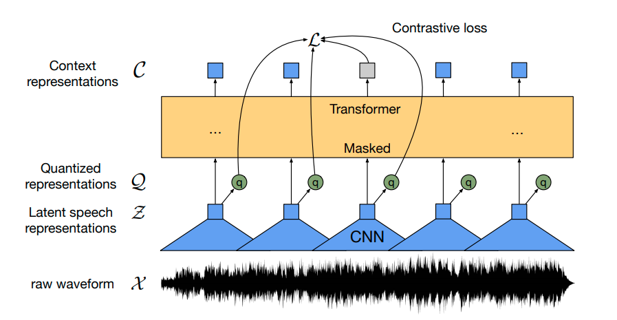
Using a novel contrastive pretraining objective, Wav2Vec2 learns powerful speech representations from more than 50.000 hours of unlabeled speech. Similar, to BERT's masked language modeling, the model learns contextualized speech representations by randomly masking feature vectors before passing them to a transformer network.
For the first time, it has been shown that pretraining, followed by fine-tuning on very little labeled speech data achieves competitive results to state-of-the-art ASR systems. Using as little as 10 minutes of labeled data, Wav2Vec2 yields a word error rate (WER) of less than 5% on the clean test set of LibriSpeech - cf. with Table 9 of the paper.
In this notebook, we will give an in-detail explanation of how Wav2Vec2's pretrained checkpoints can be fine-tuned on any English ASR dataset. Note that in this notebook, we will fine-tune Wav2Vec2 without making use of a language model. It is much simpler to use Wav2Vec2 without a language model as an end-to-end ASR system and it has been shown that a standalone Wav2Vec2 acoustic model achieves impressive results. For demonstration purposes, we fine-tune the "base"-sized pretrained checkpoint on the rather small Timit dataset that contains just 5h of training data.
Wav2Vec2 is fine-tuned using Connectionist Temporal Classification (CTC), which is an algorithm that is used to train neural networks for sequence-to-sequence problems and mainly in Automatic Speech Recognition and handwriting recognition.
I highly recommend reading the blog post Sequence Modeling with CTC (2017) very well-written blog post by Awni Hannun.
Before we start, let's install both datasets and transformers from
master. Also, we need the soundfile package to load audio files and
the jiwer to evaluate our fine-tuned model using the word error rate
(WER) metric .
!pip install datasets>=1.18.3
!pip install transformers==4.11.3
!pip install librosa
!pip install jiwer
Next we strongly suggest to upload your training checkpoints directly to the Hugging Face Hub while training. The Hub has integrated version control so you can be sure that no model checkpoint is getting lost during training.
To do so you have to store your authentication token from the Hugging Face website (sign up here if you haven't already!)
from huggingface_hub import notebook_login

notebook_login()
Print Output:
Login successful
Your token has been saved to /root/.huggingface/token
Authenticated through git-crendential store but this isn't the helper defined on your machine.
You will have to re-authenticate when pushing to the Hugging Face Hub. Run the following command in your terminal to set it as the default

git config --global credential.helper store
Then you need to install Git-LFS to upload your model checkpoints:
!apt install git-lfs
Timit is usually evaluated using the phoneme error rate (PER), but by far the most common metric in ASR is the word error rate (WER). To keep this notebook as general as possible we decided to evaluate the model using WER.
Prepare Data, Tokenizer, Feature Extractor
ASR models transcribe speech to text, which means that we both need a feature extractor that processes the speech signal to the model's input format, e.g. a feature vector, and a tokenizer that processes the model's output format to text.
In 🤗 Transformers, the Wav2Vec2 model is thus accompanied by both a tokenizer, called Wav2Vec2CTCTokenizer, and a feature extractor, called Wav2Vec2FeatureExtractor.
Let's start by creating the tokenizer responsible for decoding the model's predictions.
Create Wav2Vec2CTCTokenizer
The pretrained Wav2Vec2 checkpoint maps the speech signal to a sequence of context representations as illustrated in the figure above. A fine-tuned Wav2Vec2 checkpoint needs to map this sequence of context representations to its corresponding transcription so that a linear layer has to be added on top of the transformer block (shown in yellow). This linear layer is used to classifies each context representation to a token class analogous how, e.g., after pretraining a linear layer is added on top of BERT's embeddings for further classification - cf. with "BERT" section of this blog post.
The output size of this layer corresponds to the number of tokens in the vocabulary, which does not depend on Wav2Vec2's pretraining task, but only on the labeled dataset used for fine-tuning. So in the first step, we will take a look at Timit and define a vocabulary based on the dataset's transcriptions.
Let's start by loading the dataset and taking a look at its structure.
from datasets import load_dataset, load_metric

timit = load_dataset("timit_asr")

print(timit)
Print Output:
    DatasetDict({
        train: Dataset({
            features: ['file', 'audio', 'text', 'phonetic_detail', 'word_detail', 'dialect_region', 'sentence_type', 'speaker_id', 'id'],
            num_rows: 4620
        })
        test: Dataset({
            features: ['file', 'audio', 'text', 'phonetic_detail', 'word_detail', 'dialect_region', 'sentence_type', 'speaker_id', 'id'],
            num_rows: 1680
        })
    })
Many ASR datasets only provide the target text, 'text' for each audio
file 'file'. Timit actually provides much more information about each
audio file, such as the 'phonetic_detail', etc., which is why many
researchers choose to evaluate their models on phoneme classification
instead of speech recognition when working with Timit. However, we want
to keep the notebook as general as possible, so that we will only
consider the transcribed text for fine-tuning.
timit = timit.remove_columns(["phonetic_detail", "word_detail", "dialect_region", "id", "sentence_type", "speaker_id"])
Let's write a short function to display some random samples of the dataset and run it a couple of times to get a feeling for the transcriptions.
from datasets import ClassLabel
import random
import pandas as pd
from IPython.display import display, HTML

def show_random_elements(dataset, num_examples=10):
    assert num_examples <= len(dataset), "Can't pick more elements than there are in the dataset."
    picks = []
    for _ in range(num_examples):
        pick = random.randint(0, len(dataset)-1)
        while pick in picks:
            pick = random.randint(0, len(dataset)-1)
        picks.append(pick)

    df = pd.DataFrame(dataset[picks])
    display(HTML(df.to_html()))

show_random_elements(timit["train"].remove_columns(["file", "audio"]))
Print Output:
| Idx | Transcription |
|---|---|
| 1 | Who took the kayak down the bayou? |
| 2 | As such it acts as an anchor for the people. |
| 3 | She had your dark suit in greasy wash water all year. |
| 4 | We're not drunkards, she said. |
| 5 | The most recent geological survey found seismic activity. |
| 6 | Alimony harms a divorced man's wealth. |
| 7 | Our entire economy will have a terrific uplift. |
| 8 | Don't ask me to carry an oily rag like that. |
| 9 | The gorgeous butterfly ate a lot of nectar. |
| 10 | Where're you takin' me? |
Alright! The transcriptions look very clean and the language seems to correspond more to written text than dialogue. This makes sense taking into account that Timit is a read speech corpus.
We can see that the transcriptions contain some special characters, such
as ,.?!;:. Without a language model, it is much harder to classify
speech chunks to such special characters because they don't really
correspond to a characteristic sound unit. E.g., the letter "s" has
a more or less clear sound, whereas the special character "." does
not. Also in order to understand the meaning of a speech signal, it is
usually not necessary to include special characters in the
transcription.
In addition, we normalize the text to only have lower case letters.
import re
chars_to_ignore_regex = '[\,\?\.\!\-\;\:\"]'

def remove_special_characters(batch):
    batch["text"] = re.sub(chars_to_ignore_regex, '', batch["text"]).lower()
    return batch

timit = timit.map(remove_special_characters)
Let's take a look at the preprocessed transcriptions.
show_random_elements(timit["train"].remove_columns(["file", "audio"]))
Print Output:
| Idx | Transcription |
|---|---|
| 1 | anyhow it was high time the boy was salted |
| 2 | their basis seems deeper than mere authority |
| 3 | only the best players enjoy popularity |
| 4 | tornados often destroy acres of farm land |
| 5 | where're you takin' me |
| 6 | soak up local color |
| 7 | satellites sputniks rockets balloons what next |
| 8 | i gave them several choices and let them set the priorities |
| 9 | reading in poor light gives you eyestrain |
| 10 | that dog chases cats mercilessly |
Good! This looks better. We have removed most special characters from transcriptions and normalized them to lower-case only.
In CTC, it is common to classify speech chunks into letters, so we will do the same here. Let's extract all distinct letters of the training and test data and build our vocabulary from this set of letters.
We write a mapping function that concatenates all transcriptions into
one long transcription and then transforms the string into a set of
chars. It is important to pass the argument batched=True to the
map(...) function so that the mapping function has access to all
transcriptions at once.
def extract_all_chars(batch):
  all_text = " ".join(batch["text"])
  vocab = list(set(all_text))
  return {"vocab": [vocab], "all_text": [all_text]}

vocabs = timit.map(extract_all_chars, batched=True, batch_size=-1, keep_in_memory=True, remove_columns=timit.column_names["train"])
Now, we create the union of all distinct letters in the training dataset and test dataset and convert the resulting list into an enumerated dictionary.
vocab_list = list(set(vocabs["train"]["vocab"][0]) | set(vocabs["test"]["vocab"][0]))

vocab_dict = {v: k for k, v in enumerate(vocab_list)}
vocab_dict
Print Output:
{
     ' ': 21,
     "'": 13,
     'a': 24,
     'b': 17,
     'c': 25,
     'd': 2,
     'e': 9,
     'f': 14,
     'g': 22,
     'h': 8,
     'i': 4,
     'j': 18,
     'k': 5,
     'l': 16,
     'm': 6,
     'n': 7,
     'o': 10,
     'p': 19,
     'q': 3,
     'r': 20,
     's': 11,
     't': 0,
     'u': 26,
     'v': 27,
     'w': 1,
     'x': 23,
     'y': 15,
     'z': 12
}
Cool, we see that all letters of the alphabet occur in the dataset
(which is not really surprising) and we also extracted the special
characters " " and '. Note that we did not exclude those special
characters because:
- The model has to learn to predict when a word finished or else the model prediction would always be a sequence of chars which would make it impossible to separate words from each other.
- In English, we need to keep the
'character to differentiate between words, e.g.,"it's"and"its"which have very different meanings.
To make it clearer that " " has its own token class, we give it a more
visible character |. In addition, we also add an "unknown" token so
that the model can later deal with characters not encountered in
Timit's training set.
vocab_dict["|"] = vocab_dict[" "]
del vocab_dict[" "]
Finally, we also add a padding token that corresponds to CTC's "blank token". The "blank token" is a core component of the CTC algorithm. For more information, please take a look at the "Alignment" section here.
vocab_dict["[UNK]"] = len(vocab_dict)
vocab_dict["[PAD]"] = len(vocab_dict)
print(len(vocab_dict))
Print Output:
30
Cool, now our vocabulary is complete and consists of 30 tokens, which means that the linear layer that we will add on top of the pretrained Wav2Vec2 checkpoint will have an output dimension of 30.
Let's now save the vocabulary as a json file.
import json
with open('vocab.json', 'w') as vocab_file:
    json.dump(vocab_dict, vocab_file)
In a final step, we use the json file to instantiate an object of the
Wav2Vec2CTCTokenizer class.
from transformers import Wav2Vec2CTCTokenizer

tokenizer = Wav2Vec2CTCTokenizer("./vocab.json", unk_token="[UNK]", pad_token="[PAD]", word_delimiter_token="|")
If one wants to re-use the just created tokenizer with the fine-tuned model of this notebook, it is strongly advised to upload the tokenizer to the 🤗 Hub. Let's call the repo to which we will upload the files
"wav2vec2-large-xlsr-turkish-demo-colab":
repo_name = "wav2vec2-base-timit-demo-colab"
and upload the tokenizer to the 🤗 Hub.
tokenizer.push_to_hub(repo_name)
Great, you can see the just created repository under https://huggingface.co/<your-username>/wav2vec2-base-timit-demo-colab
Create Wav2Vec2 Feature Extractor
Speech is a continuous signal and to be treated by computers, it first has to be discretized, which is usually called sampling. The sampling rate hereby plays an important role in that it defines how many data points of the speech signal are measured per second. Therefore, sampling with a higher sampling rate results in a better approximation of the real speech signal but also necessitates more values per second.
A pretrained checkpoint expects its input data to have been sampled more or less from the same distribution as the data it was trained on. The same speech signals sampled at two different rates have a very different distribution, e.g., doubling the sampling rate results in data points being twice as long. Thus, before fine-tuning a pretrained checkpoint of an ASR model, it is crucial to verify that the sampling rate of the data that was used to pretrain the model matches the sampling rate of the dataset used to fine-tune the model.
Wav2Vec2 was pretrained on the audio data of LibriSpeech and LibriVox which both were sampling with 16kHz. Our fine-tuning dataset, Timit, was luckily also sampled with 16kHz. If the fine-tuning dataset would have been sampled with a rate lower or higher than 16kHz, we first would have had to up or downsample the speech signal to match the sampling rate of the data used for pretraining.
A Wav2Vec2 feature extractor object requires the following parameters to be instantiated:
feature_size: Speech models take a sequence of feature vectors as an input. While the length of this sequence obviously varies, the feature size should not. In the case of Wav2Vec2, the feature size is 1 because the model was trained on the raw speech signal .sampling_rate: The sampling rate at which the model is trained on.padding_value: For batched inference, shorter inputs need to be padded with a specific valuedo_normalize: Whether the input should be zero-mean-unit-variance normalized or not. Usually, speech models perform better when normalizing the inputreturn_attention_mask: Whether the model should make use of anattention_maskfor batched inference. In general, models should always make use of theattention_maskto mask padded tokens. However, due to a very specific design choice ofWav2Vec2's "base" checkpoint, better results are achieved when using noattention_mask. This is not recommended for other speech models. For more information, one can take a look at this issue. Important If you want to use this notebook to fine-tune large-lv60, this parameter should be set toTrue.
from transformers import Wav2Vec2FeatureExtractor

feature_extractor = Wav2Vec2FeatureExtractor(feature_size=1, sampling_rate=16000, padding_value=0.0, do_normalize=True, return_attention_mask=False)
Great, Wav2Vec2's feature extraction pipeline is thereby fully defined!
To make the usage of Wav2Vec2 as user-friendly as possible, the feature
extractor and tokenizer are wrapped into a single Wav2Vec2Processor
class so that one only needs a model and processor object.
from transformers import Wav2Vec2Processor

processor = Wav2Vec2Processor(feature_extractor=feature_extractor, tokenizer=tokenizer)
Preprocess Data
So far, we have not looked at the actual values of the speech signal but just the transcription. In addition to sentence, our datasets include two more column names path and audio. path states the absolute path of the audio file. Let's take a look.
print(timit[0]["path"])
Print Output:
'/root/.cache/huggingface/datasets/downloads/extracted/404950a46da14eac65eb4e2a8317b1372fb3971d980d91d5d5b221275b1fd7e0/data/TRAIN/DR4/MMDM0/SI681.WAV'
Wav2Vec2 expects the input in the format of a 1-dimensional array of 16 kHz. This means that the audio file has to be loaded and resampled.
Thankfully, datasets does this automatically by calling the other column audio. Let try it out.
common_voice_train[0]["audio"]
Print Output:
{'array': array([-2.1362305e-04,  6.1035156e-05,  3.0517578e-05, ...,
        -3.0517578e-05, -9.1552734e-05, -6.1035156e-05], dtype=float32),
 'path': '/root/.cache/huggingface/datasets/downloads/extracted/404950a46da14eac65eb4e2a8317b1372fb3971d980d91d5d5b221275b1fd7e0/data/TRAIN/DR4/MMDM0/SI681.WAV',
 'sampling_rate': 16000}
We can see that the audio file has automatically been loaded. This is thanks to the new "Audio" feature introduced in datasets == 4.13.3, which loads and resamples audio files on-the-fly upon calling.
The sampling rate is set to 16kHz which is what Wav2Vec2 expects as an input.
Great, let's listen to a couple of audio files to better understand the dataset and verify that the audio was correctly loaded.
import IPython.display as ipd
import numpy as np
import random

rand_int = random.randint(0, len(timit["train"]))

print(timit["train"][rand_int]["text"])
ipd.Audio(data=np.asarray(timit["train"][rand_int]["audio"]["array"]), autoplay=True, rate=16000)
It can be heard, that the speakers change along with their speaking rate, accent, etc. Overall, the recordings sound relatively clear though, which is to be expected from a read speech corpus.
Let's do a final check that the data is correctly prepared, by printing the shape of the speech input, its transcription, and the corresponding sampling rate.
rand_int = random.randint(0, len(timit["train"]))

print("Target text:", timit["train"][rand_int]["text"])
print("Input array shape:", np.asarray(timit["train"][rand_int]["audio"]["array"]).shape)
print("Sampling rate:", timit["train"][rand_int]["audio"]["sampling_rate"])
Print Output:
    Target text: she had your dark suit in greasy wash water all year
    Input array shape: (52941,)
    Sampling rate: 16000
Good! Everything looks fine - the data is a 1-dimensional array, the sampling rate always corresponds to 16kHz, and the target text is normalized.
Finally, we can process the dataset to the format expected by the model for training. We will make use of the map(...) function.
First, we load and resample the audio data, simply by calling batch["audio"].
Second, we extract the input_values from the loaded audio file. In our case, the Wav2Vec2Processor only normalizes the data. For other speech models, however, this step can include more complex feature extraction, such as Log-Mel feature extraction.
Third, we encode the transcriptions to label ids.
Note: This mapping function is a good example of how the Wav2Vec2Processor class should be used. In "normal" context, calling processor(...) is redirected to Wav2Vec2FeatureExtractor's call method. When wrapping the processor into the as_target_processor context, however, the same method is redirected to Wav2Vec2CTCTokenizer's call method.
For more information please check the docs.
def prepare_dataset(batch):
    audio = batch["audio"]

    # batched output is "un-batched" to ensure mapping is correct
    batch["input_values"] = processor(audio["array"], sampling_rate=audio["sampling_rate"]).input_values[0]

    with processor.as_target_processor():
        batch["labels"] = processor(batch["text"]).input_ids
    return batch
Let's apply the data preparation function to all examples.
timit = timit.map(prepare_dataset, remove_columns=timit.column_names["train"], num_proc=4)
Note: Currently datasets make use of torchaudio and librosa for audio loading and resampling. If you wish to implement your own costumized data loading/sampling, feel free to just make use of the "path" column instead and disregard the "audio" column.
Training & Evaluation
The data is processed so that we are ready to start setting up the training pipeline. We will make use of 🤗's Trainer for which we essentially need to do the following:
Define a data collator. In contrast to most NLP models, Wav2Vec2 has a much larger input length than output length. E.g., a sample of input length 50000 has an output length of no more than 100. Given the large input sizes, it is much more efficient to pad the training batches dynamically meaning that all training samples should only be padded to the longest sample in their batch and not the overall longest sample. Therefore, fine-tuning Wav2Vec2 requires a special padding data collator, which we will define below
Evaluation metric. During training, the model should be evaluated on the word error rate. We should define a
compute_metricsfunction accordinglyLoad a pretrained checkpoint. We need to load a pretrained checkpoint and configure it correctly for training.
Define the training configuration.
After having fine-tuned the model, we will correctly evaluate it on the test data and verify that it has indeed learned to correctly transcribe speech.
Set-up Trainer
Let's start by defining the data collator. The code for the data collator was copied from this example.
Without going into too many details, in contrast to the common data
collators, this data collator treats the input_values and labels
differently and thus applies to separate padding functions on them
(again making use of Wav2Vec2's context manager). This is necessary
because in speech input and output are of different modalities meaning
that they should not be treated by the same padding function. Analogous
to the common data collators, the padding tokens in the labels with
-100 so that those tokens are not taken into account when
computing the loss.
import torch

from dataclasses import dataclass, field
from typing import Any, Dict, List, Optional, Union

@dataclass
class DataCollatorCTCWithPadding:
    """
    Data collator that will dynamically pad the inputs received.
    Args:
        processor (:class:`~transformers.Wav2Vec2Processor`)
            The processor used for proccessing the data.
        padding (:obj:`bool`, :obj:`str` or :class:`~transformers.tokenization_utils_base.PaddingStrategy`, `optional`, defaults to :obj:`True`):
            Select a strategy to pad the returned sequences (according to the model's padding side and padding index)
            among:
            * :obj:`True` or :obj:`'longest'`: Pad to the longest sequence in the batch (or no padding if only a single
              sequence if provided).
            * :obj:`'max_length'`: Pad to a maximum length specified with the argument :obj:`max_length` or to the
              maximum acceptable input length for the model if that argument is not provided.
            * :obj:`False` or :obj:`'do_not_pad'` (default): No padding (i.e., can output a batch with sequences of
              different lengths).
        max_length (:obj:`int`, `optional`):
            Maximum length of the ``input_values`` of the returned list and optionally padding length (see above).
        max_length_labels (:obj:`int`, `optional`):
            Maximum length of the ``labels`` returned list and optionally padding length (see above).
        pad_to_multiple_of (:obj:`int`, `optional`):
            If set will pad the sequence to a multiple of the provided value.
            This is especially useful to enable the use of Tensor Cores on NVIDIA hardware with compute capability >=
            7.5 (Volta).
    """

    processor: Wav2Vec2Processor
    padding: Union[bool, str] = True
    max_length: Optional[int] = None
    max_length_labels: Optional[int] = None
    pad_to_multiple_of: Optional[int] = None
    pad_to_multiple_of_labels: Optional[int] = None

    def __call__(self, features: List[Dict[str, Union[List[int], torch.Tensor]]]) -> Dict[str, torch.Tensor]:
        # split inputs and labels since they have to be of different lengths and need
        # different padding methods
        input_features = [{"input_values": feature["input_values"]} for feature in features]
        label_features = [{"input_ids": feature["labels"]} for feature in features]

        batch = self.processor.pad(
            input_features,
            padding=self.padding,
            max_length=self.max_length,
            pad_to_multiple_of=self.pad_to_multiple_of,
            return_tensors="pt",
        )
        with self.processor.as_target_processor():
            labels_batch = self.processor.pad(
                label_features,
                padding=self.padding,
                max_length=self.max_length_labels,
                pad_to_multiple_of=self.pad_to_multiple_of_labels,
                return_tensors="pt",
            )

        # replace padding with -100 to ignore loss correctly
        labels = labels_batch["input_ids"].masked_fill(labels_batch.attention_mask.ne(1), -100)

        batch["labels"] = labels

        return batch
Let's initialize the data collator.
data_collator = DataCollatorCTCWithPadding(processor=processor, padding=True)
Next, the evaluation metric is defined. As mentioned earlier, the predominant metric in ASR is the word error rate (WER), hence we will use it in this notebook as well.
wer_metric = load_metric("wer")
The model will return a sequence of logit vectors:
,
with and .
A logit vector contains the log-odds for each word in the
vocabulary we defined earlier, thus
config.vocab_size. We are interested in the most likely prediction of
the model and thus take the argmax(...) of the logits. Also, we
transform the encoded labels back to the original string by replacing
-100 with the pad_token_id and decoding the ids while making sure
that consecutive tokens are not grouped to the same token in CTC
style .
def compute_metrics(pred):
    pred_logits = pred.predictions
    pred_ids = np.argmax(pred_logits, axis=-1)

    pred.label_ids[pred.label_ids == -100] = processor.tokenizer.pad_token_id

    pred_str = processor.batch_decode(pred_ids)
    # we do not want to group tokens when computing the metrics
    label_str = processor.batch_decode(pred.label_ids, group_tokens=False)

    wer = wer_metric.compute(predictions=pred_str, references=label_str)

    return {"wer": wer}
Now, we can load the pretrained Wav2Vec2 checkpoint. The tokenizer's
pad_token_id must be to define the model's pad_token_id or in the
case of Wav2Vec2ForCTC also CTC's blank token . To save GPU
memory, we enable PyTorch's gradient
checkpointing and also
set the loss reduction to "mean".
from transformers import Wav2Vec2ForCTC

model = Wav2Vec2ForCTC.from_pretrained(
    "facebook/wav2vec2-base",
    ctc_loss_reduction="mean",
    pad_token_id=processor.tokenizer.pad_token_id,
)
Print Output:
    Some weights of Wav2Vec2ForCTC were not initialized from the model checkpoint at facebook/wav2vec2-base and are newly initialized: ['lm_head.weight', 'lm_head.bias']
    You should probably TRAIN this model on a down-stream task to be able to use it for predictions and inference.
The first component of Wav2Vec2 consists of a stack of CNN layers that
are used to extract acoustically meaningful - but contextually
independent - features from the raw speech signal. This part of the
model has already been sufficiently trained during pretrainind and as
stated in the paper does not need to
be fine-tuned anymore. Thus, we can set the requires_grad to False
for all parameters of the feature extraction part.
model.freeze_feature_extractor()
In a final step, we define all parameters related to training. To give more explanation on some of the parameters:
group_by_lengthmakes training more efficient by grouping training samples of similar input length into one batch. This can significantly speed up training time by heavily reducing the overall number of useless padding tokens that are passed through the modellearning_rateandweight_decaywere heuristically tuned until fine-tuning has become stable. Note that those parameters strongly depend on the Timit dataset and might be suboptimal for other speech datasets.
For more explanations on other parameters, one can take a look at the docs.
During training, a checkpoint will be uploaded asynchronously to the hub every 400 training steps. It allows you to also play around with the demo widget even while your model is still training.
Note: If one does not want to upload the model checkpoints to the hub, simply set push_to_hub=False.
from transformers import TrainingArguments

training_args = TrainingArguments(
  output_dir=repo_name,
  group_by_length=True,
  per_device_train_batch_size=32,
  evaluation_strategy="steps",
  num_train_epochs=30,
  fp16=True,
  gradient_checkpointing=True,
  save_steps=500,
  eval_steps=500,
  logging_steps=500,
  learning_rate=1e-4,
  weight_decay=0.005,
  warmup_steps=1000,
  save_total_limit=2,
)
Now, all instances can be passed to Trainer and we are ready to start training!
from transformers import Trainer

trainer = Trainer(
    model=model,
    data_collator=data_collator,
    args=training_args,
    compute_metrics=compute_metrics,
    train_dataset=timit_prepared["train"],
    eval_dataset=timit_prepared["test"],
    tokenizer=processor.feature_extractor,
)
To allow models to become independent of the speaker rate, in
CTC, consecutive tokens that are identical are simply grouped as a
single token. However, the encoded labels should not be grouped when
decoding since they don't correspond to the predicted tokens of the
model, which is why the group_tokens=False parameter has to be passed.
If we wouldn't pass this parameter a word like "hello" would
incorrectly be encoded, and decoded as "helo".
The blank token allows the model to predict a word, such as
"hello" by forcing it to insert the blank token between the two l's.
A CTC-conform prediction of "hello" of our model would be
[PAD] [PAD] "h" "e" "e" "l" "l" [PAD] "l" "o" "o" [PAD].
Training
Training will take between 90 and 180 minutes depending on the GPU allocated to the google colab attached to this notebook. While the trained model yields satisfying results on Timit's test data, it is by no means an optimally fine-tuned model. The purpose of this notebook is to demonstrate how Wav2Vec2's base, large, and large-lv60 checkpoints can be fine-tuned on any English dataset.
In case you want to use this google colab to fine-tune your model, you should make sure that your training doesn't stop due to inactivity. A simple hack to prevent this is to paste the following code into the console of this tab (right mouse click -> inspect -> Console tab and insert code).
function ConnectButton(){
    console.log("Connect pushed");
    document.querySelector("#top-toolbar > colab-connect-button").shadowRoot.querySelector("#connect").click()
}
setInterval(ConnectButton,60000);
trainer.train()
Depending on your GPU, it might be possible that you are seeing an "out-of-memory" error here. In this case, it's probably best to reduce per_device_train_batch_size to 16 or even less and eventually make use of gradient_accumulation.
Print Output:
| Step | Training Loss | Validation Loss | WER | Runtime | Samples per Second |
|---|---|---|---|---|---|
| 500 | 3.758100 | 1.686157 | 0.945214 | 97.299000 | 17.266000 |
| 1000 | 0.691400 | 0.476487 | 0.391427 | 98.283300 | 17.093000 |
| 1500 | 0.202400 | 0.403425 | 0.330715 | 99.078100 | 16.956000 |
| 2000 | 0.115200 | 0.405025 | 0.307353 | 98.116500 | 17.122000 |
| 2500 | 0.075000 | 0.428119 | 0.294053 | 98.496500 | 17.056000 |
| 3000 | 0.058200 | 0.442629 | 0.287299 | 98.871300 | 16.992000 |
| 3500 | 0.047600 | 0.442619 | 0.285783 | 99.477500 | 16.888000 |
| 4000 | 0.034500 | 0.456989 | 0.282200 | 99.419100 | 16.898000 |
The final WER should be below 0.3 which is reasonable given that state-of-the-art phoneme error rates (PER) are just below 0.1 (see leaderboard) and that WER is usually worse than PER.
You can now upload the result of the training to the Hub, just execute this instruction:
trainer.push_to_hub()
You can now share this model with all your friends, family, favorite pets: they can all load it with the identifier "your-username/the-name-you-picked" so for instance:
from transformers import AutoModelForCTC, Wav2Vec2Processor

model = AutoModelForCTC.from_pretrained("patrickvonplaten/wav2vec2-base-timit-demo-colab")
processor = Wav2Vec2Processor.from_pretrained("patrickvonplaten/wav2vec2-base-timit-demo-colab")
Evaluation
In the final part, we evaluate our fine-tuned model on the test set and play around with it a bit.
Let's load the processor and model.
processor = Wav2Vec2Processor.from_pretrained(repo_name)
model = Wav2Vec2ForCTC.from_pretrained(repo_name)
Now, we will make use of the map(...) function to predict the
transcription of every test sample and to save the prediction in the
dataset itself. We will call the resulting dictionary "results".
Note: we evaluate the test data set with batch_size=1 on purpose
due to this issue.
Since padded inputs don't yield the exact same output as non-padded
inputs, a better WER can be achieved by not padding the input at all.
def map_to_result(batch):
  with torch.no_grad():
    input_values = torch.tensor(batch["input_values"], device="cuda").unsqueeze(0)
    logits = model(input_values).logits

  pred_ids = torch.argmax(logits, dim=-1)
  batch["pred_str"] = processor.batch_decode(pred_ids)[0]
  batch["text"] = processor.decode(batch["labels"], group_tokens=False)

  return batch

results = timit["test"].map(map_to_result, remove_columns=timit["test"].column_names)
Let's compute the overall WER now.
print("Test WER: {:.3f}".format(wer_metric.compute(predictions=results["pred_str"], references=results["text"])))
Print Output:
Test WER: 0.221
22.1% WER - not bad! Our demo model would have probably made it on the official leaderboard.
Let's take a look at some predictions to see what errors are made by the model.
Print Output:
show_random_elements(results.remove_columns(["speech", "sampling_rate"]))
| pred_str | target_text |
|---|---|
| am to balence your employe you benefits package | aim to balance your employee benefit package |
| the fawlg prevented them from ariving on tom | the fog prevented them from arriving on time |
| young children should avoide exposure to contagieous diseases | young children should avoid exposure to contagious diseases |
| artifficial intelligence is for real | artificial intelligence is for real |
| their pcrops were two step latters a chair and a polmb fan | their props were two stepladders a chair and a palm fan |
| if people were more generous there would be no need for wealfare | if people were more generous there would be no need for welfare |
| the fish began to leep frantically on the surface of the small ac | the fish began to leap frantically on the surface of the small lake |
| her right hand eggs whenever the barametric pressur changes | her right hand aches whenever the barometric pressure changes |
| only lawyers loved miliunears | only lawyers love millionaires |
| the nearest cennagade may not be within wallkin distance | the nearest synagogue may not be within walking distance |
It becomes clear that the predicted transcriptions are acoustically very similar to the target transcriptions, but often contain spelling or grammatical errors. This shouldn't be very surprising though given that we purely rely on Wav2Vec2 without making use of a language model.
Finally, to better understand how CTC works, it is worth taking a deeper look at the exact output of the model. Let's run the first test sample through the model, take the predicted ids and convert them to their corresponding tokens.
model.to("cuda")

with torch.no_grad():
  logits = model(torch.tensor(timit["test"][:1]["input_values"], device="cuda")).logits

pred_ids = torch.argmax(logits, dim=-1)

# convert ids to tokens
" ".join(processor.tokenizer.convert_ids_to_tokens(pred_ids[0].tolist()))
Print Output:
[PAD] [PAD] [PAD] [PAD] [PAD] [PAD] t t h e e | | b b [PAD] u u n n n g g [PAD] a [PAD] [PAD] l l [PAD] o o o [PAD] | w w a a [PAD] s s | | [PAD] [PAD] p l l e e [PAD] [PAD] s s e n n t t t [PAD] l l y y | | | s s [PAD] i i [PAD] t t t [PAD] u u u u [PAD] [PAD] [PAD] a a [PAD] t t e e e d d d | n n e e a a a r | | t h h e | | s s h h h [PAD] o o o [PAD] o o r r [PAD] [PAD] [PAD] [PAD] [PAD] [PAD] [PAD] [PAD] [PAD] [PAD] [PAD]
The output should make it a bit clearer how CTC works in practice. The model is to some extent invariant to speaking rate since it has learned to either just repeat the same token in case the speech chunk to be classified still corresponds to the same token. This makes CTC a very powerful algorithm for speech recognition since the speech file's transcription is often very much independent of its length.
I again advise the reader to take a look at this very nice blog post to better understand CTC.