The Annotated Diffusion Model


In this blog post, we'll take a deeper look into Denoising Diffusion Probabilistic Models (also known as DDPMs, diffusion models, score-based generative models or simply autoencoders) as researchers have been able to achieve remarkable results with them for (un)conditional image/audio/video generation. Popular examples (at the time of writing) include GLIDE and DALL-E 2 by OpenAI, Latent Diffusion by the University of Heidelberg and ImageGen by Google Brain.
We'll go over the original DDPM paper by (Ho et al., 2020), implementing it step-by-step in PyTorch, based on Phil Wang's implementation - which itself is based on the original TensorFlow implementation. Note that the idea of diffusion for generative modeling was actually already introduced in (Sohl-Dickstein et al., 2015). However, it took until (Song et al., 2019) (at Stanford University), and then (Ho et al., 2020) (at Google Brain) who independently improved the approach.
Note that there are several perspectives on diffusion models. Here, we employ the discrete-time (latent variable model) perspective, but be sure to check out the other perspectives as well.
Alright, let's dive in!
from IPython.display import Image
Image(filename='assets/78_annotated-diffusion/ddpm_paper.png')
We'll install and import the required libraries first (assuming you have PyTorch installed).
!pip install -q -U einops datasets matplotlib tqdm

import math
from inspect import isfunction
from functools import partial

%matplotlib inline
import matplotlib.pyplot as plt
from tqdm.auto import tqdm
from einops import rearrange, reduce
from einops.layers.torch import Rearrange

import torch
from torch import nn, einsum
import torch.nn.functional as F
What is a diffusion model?
A (denoising) diffusion model isn't that complex if you compare it to other generative models such as Normalizing Flows, GANs or VAEs: they all convert noise from some simple distribution to a data sample. This is also the case here where a neural network learns to gradually denoise data starting from pure noise.
In a bit more detail for images, the set-up consists of 2 processes:
- a fixed (or predefined) forward diffusion process of our choosing, that gradually adds Gaussian noise to an image, until you end up with pure noise
- a learned reverse denoising diffusion process , where a neural network is trained to gradually denoise an image starting from pure noise, until you end up with an actual image.
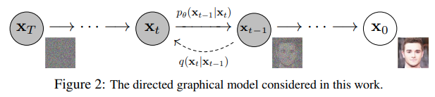
Both the forward and reverse process indexed by happen for some number of finite time steps (the DDPM authors use ). You start with where you sample a real image from your data distribution (let's say an image of a cat from ImageNet), and the forward process samples some noise from a Gaussian distribution at each time step , which is added to the image of the previous time step. Given a sufficiently large and a well behaved schedule for adding noise at each time step, you end up with what is called an isotropic Gaussian distribution at via a gradual process.
In more mathematical form
Let's write this down more formally, as ultimately we need a tractable loss function which our neural network needs to optimize.
Let be the real data distribution, say of "real images". We can sample from this distribution to get an image, . We define the forward diffusion process which adds Gaussian noise at each time step , according to a known variance schedule as
Recall that a normal distribution (also called Gaussian distribution) is defined by 2 parameters: a mean and a variance . Basically, each new (slightly noisier) image at time step is drawn from a conditional Gaussian distribution with and , which we can do by sampling and then setting .
Note that the aren't constant at each time step (hence the subscript) --- in fact one defines a so-called "variance schedule", which can be linear, quadratic, cosine, etc. as we will see further (a bit like a learning rate schedule).
So starting from , we end up with , where is pure Gaussian noise if we set the schedule appropriately.
Now, if we knew the conditional distribution , then we could run the process in reverse: by sampling some random Gaussian noise , and then gradually "denoise" it so that we end up with a sample from the real distribution .
However, we don't know . It's intractable since it requires knowing the distribution of all possible images in order to calculate this conditional probability. Hence, we're going to leverage a neural network to approximate (learn) this conditional probability distribution, let's call it , with being the parameters of the neural network, updated by gradient descent.
Ok, so we need a neural network to represent a (conditional) probability distribution of the backward process. If we assume this reverse process is Gaussian as well, then recall that any Gaussian distribution is defined by 2 parameters:
- a mean parametrized by ;
- a variance parametrized by ;
so we can parametrize the process as where the mean and variance are also conditioned on the noise level .
Hence, our neural network needs to learn/represent the mean and variance. However, the DDPM authors decided to keep the variance fixed, and let the neural network only learn (represent) the mean of this conditional probability distribution. From the paper:
First, we set to untrained time dependent constants. Experimentally, both and (see paper) had similar results.
This was then later improved in the Improved diffusion models paper, where a neural network also learns the variance of this backwards process, besides the mean.
So we continue, assuming that our neural network only needs to learn/represent the mean of this conditional probability distribution.
Defining an objective function (by reparametrizing the mean)
To derive an objective function to learn the mean of the backward process, the authors observe that the combination of and can be seen as a variational auto-encoder (VAE) (Kingma et al., 2013). Hence, the variational lower bound (also called ELBO) can be used to minimize the negative log-likelihood with respect to ground truth data sample (we refer to the VAE paper for details regarding ELBO). It turns out that the ELBO for this process is a sum of losses at each time step , . By construction of the forward process and backward process, each term (except for ) of the loss is actually the KL divergence between 2 Gaussian distributions which can be written explicitly as an L2-loss with respect to the means!
A direct consequence of the constructed forward process , as shown by Sohl-Dickstein et al., is that we can sample at any arbitrary noise level conditioned on (since sums of Gaussians is also Gaussian). This is very convenient: we don't need to apply repeatedly in order to sample . We have that
with and . Let's refer to this equation as the "nice property". This means we can sample Gaussian noise and scale it appropriatly and add it to to get directly. Note that the are functions of the known variance schedule and thus are also known and can be precomputed. This then allows us, during training, to optimize random terms of the loss function (or in other words, to randomly sample during training and optimize ).
Another beauty of this property, as shown in Ho et al. is that one can (after some math, for which we refer the reader to this excellent blog post) instead reparametrize the mean to make the neural network learn (predict) the added noise (via a network ) for noise level in the KL terms which constitute the losses. This means that our neural network becomes a noise predictor, rather than a (direct) mean predictor. The mean can be computed as follows:
The final objective function then looks as follows (for a random time step given ):
Here, is the initial (real, uncorrupted) image, and we see the direct noise level sample given by the fixed forward process. is the pure noise sampled at time step , and is our neural network. The neural network is optimized using a simple mean squared error (MSE) between the true and the predicted Gaussian noise.
The training algorithm now looks as follows:
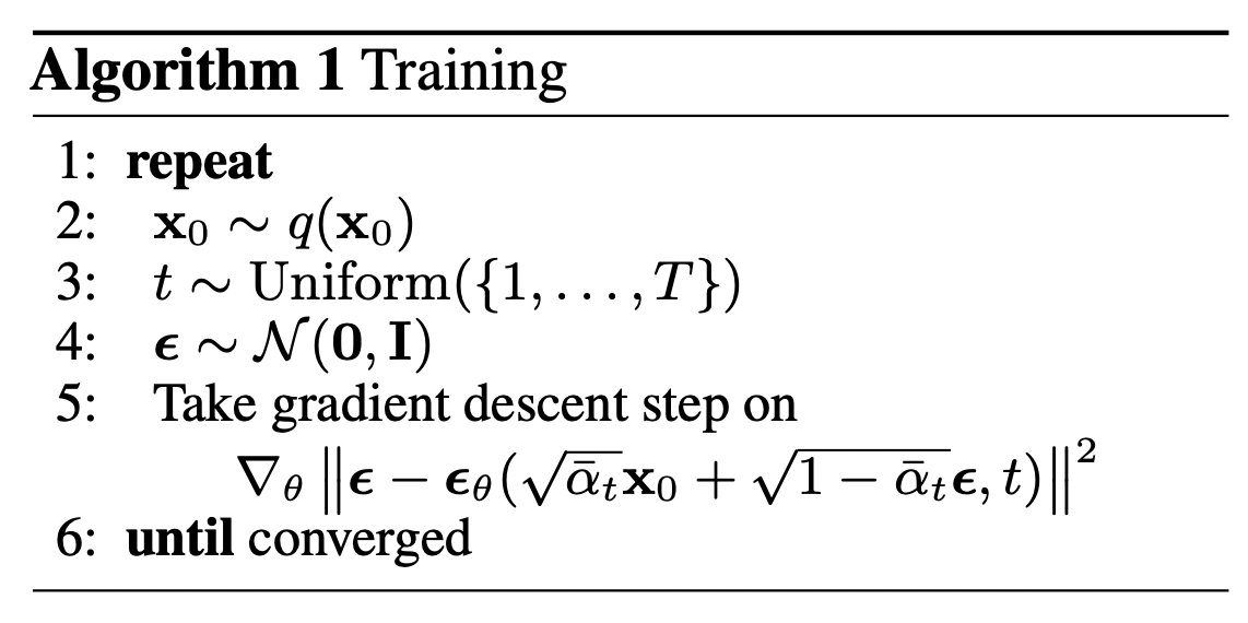
In other words:
- we take a random sample from the real unknown and possibily complex data distribution
- we sample a noise level uniformally between and (i.e., a random time step)
- we sample some noise from a Gaussian distribution and corrupt the input by this noise at level (using the nice property defined above)
- the neural network is trained to predict this noise based on the corrupted image (i.e. noise applied on based on known schedule )
In reality, all of this is done on batches of data, as one uses stochastic gradient descent to optimize neural networks.
The neural network
The neural network needs to take in a noised image at a particular time step and return the predicted noise. Note that the predicted noise is a tensor that has the same size/resolution as the input image. So technically, the network takes in and outputs tensors of the same shape. What type of neural network can we use for this?
What is typically used here is very similar to that of an Autoencoder, which you may remember from typical "intro to deep learning" tutorials. Autoencoders have a so-called "bottleneck" layer in between the encoder and decoder. The encoder first encodes an image into a smaller hidden representation called the "bottleneck", and the decoder then decodes that hidden representation back into an actual image. This forces the network to only keep the most important information in the bottleneck layer.
In terms of architecture, the DDPM authors went for a U-Net, introduced by (Ronneberger et al., 2015) (which, at the time, achieved state-of-the-art results for medical image segmentation). This network, like any autoencoder, consists of a bottleneck in the middle that makes sure the network learns only the most important information. Importantly, it introduced residual connections between the encoder and decoder, greatly improving gradient flow (inspired by ResNet in He et al., 2015).
As can be seen, a U-Net model first downsamples the input (i.e. makes the input smaller in terms of spatial resolution), after which upsampling is performed.
Below, we implement this network, step-by-step.
Network helpers
First, we define some helper functions and classes which will be used when implementing the neural network. Importantly, we define a Residual module, which simply adds the input to the output of a particular function (in other words, adds a residual connection to a particular function).
We also define aliases for the up- and downsampling operations.
def exists(x):
    return x is not None

def default(val, d):
    if exists(val):
        return val
    return d() if isfunction(d) else d


def num_to_groups(num, divisor):
    groups = num // divisor
    remainder = num % divisor
    arr = [divisor] * groups
    if remainder > 0:
        arr.append(remainder)
    return arr


class Residual(nn.Module):
    def __init__(self, fn):
        super().__init__()
        self.fn = fn

    def forward(self, x, *args, **kwargs):
        return self.fn(x, *args, **kwargs) + x


def Upsample(dim, dim_out=None):
    return nn.Sequential(
        nn.Upsample(scale_factor=2, mode="nearest"),
        nn.Conv2d(dim, default(dim_out, dim), 3, padding=1),
    )


def Downsample(dim, dim_out=None):
    # No More Strided Convolutions or Pooling
    return nn.Sequential(
        Rearrange("b c (h p1) (w p2) -> b (c p1 p2) h w", p1=2, p2=2),
        nn.Conv2d(dim * 4, default(dim_out, dim), 1),
    )
Position embeddings
As the parameters of the neural network are shared across time (noise level), the authors employ sinusoidal position embeddings to encode , inspired by the Transformer (Vaswani et al., 2017). This makes the neural network "know" at which particular time step (noise level) it is operating, for every image in a batch.
The SinusoidalPositionEmbeddings module takes a tensor of shape (batch_size, 1) as input (i.e. the noise levels of several noisy images in a batch), and turns this into a tensor of shape (batch_size, dim), with dim being the dimensionality of the position embeddings. This is then added to each residual block, as we will see further.
class SinusoidalPositionEmbeddings(nn.Module):
    def __init__(self, dim):
        super().__init__()
        self.dim = dim

    def forward(self, time):
        device = time.device
        half_dim = self.dim // 2
        embeddings = math.log(10000) / (half_dim - 1)
        embeddings = torch.exp(torch.arange(half_dim, device=device) * -embeddings)
        embeddings = time[:, None] * embeddings[None, :]
        embeddings = torch.cat((embeddings.sin(), embeddings.cos()), dim=-1)
        return embeddings
ResNet block
Next, we define the core building block of the U-Net model. The DDPM authors employed a Wide ResNet block (Zagoruyko et al., 2016), but Phil Wang has replaced the standard convolutional layer by a "weight standardized" version, which works better in combination with group normalization (see (Kolesnikov et al., 2019) for details).
class WeightStandardizedConv2d(nn.Conv2d):
    """
    https://arxiv.org/abs/1903.10520
    weight standardization purportedly works synergistically with group normalization
    """

    def forward(self, x):
        eps = 1e-5 if x.dtype == torch.float32 else 1e-3

        weight = self.weight
        mean = reduce(weight, "o ... -> o 1 1 1", "mean")
        var = reduce(weight, "o ... -> o 1 1 1", partial(torch.var, unbiased=False))
        normalized_weight = (weight - mean) / (var + eps).rsqrt()

        return F.conv2d(
            x,
            normalized_weight,
            self.bias,
            self.stride,
            self.padding,
            self.dilation,
            self.groups,
        )


class Block(nn.Module):
    def __init__(self, dim, dim_out, groups=8):
        super().__init__()
        self.proj = WeightStandardizedConv2d(dim, dim_out, 3, padding=1)
        self.norm = nn.GroupNorm(groups, dim_out)
        self.act = nn.SiLU()

    def forward(self, x, scale_shift=None):
        x = self.proj(x)
        x = self.norm(x)

        if exists(scale_shift):
            scale, shift = scale_shift
            x = x * (scale + 1) + shift

        x = self.act(x)
        return x


class ResnetBlock(nn.Module):
    """https://arxiv.org/abs/1512.03385"""

    def __init__(self, dim, dim_out, *, time_emb_dim=None, groups=8):
        super().__init__()
        self.mlp = (
            nn.Sequential(nn.SiLU(), nn.Linear(time_emb_dim, dim_out * 2))
            if exists(time_emb_dim)
            else None
        )

        self.block1 = Block(dim, dim_out, groups=groups)
        self.block2 = Block(dim_out, dim_out, groups=groups)
        self.res_conv = nn.Conv2d(dim, dim_out, 1) if dim != dim_out else nn.Identity()

    def forward(self, x, time_emb=None):
        scale_shift = None
        if exists(self.mlp) and exists(time_emb):
            time_emb = self.mlp(time_emb)
            time_emb = rearrange(time_emb, "b c -> b c 1 1")
            scale_shift = time_emb.chunk(2, dim=1)

        h = self.block1(x, scale_shift=scale_shift)
        h = self.block2(h)
        return h + self.res_conv(x)
Attention module
Next, we define the attention module, which the DDPM authors added in between the convolutional blocks. Attention is the building block of the famous Transformer architecture (Vaswani et al., 2017), which has shown great success in various domains of AI, from NLP and vision to protein folding. Phil Wang employs 2 variants of attention: one is regular multi-head self-attention (as used in the Transformer), the other one is a linear attention variant (Shen et al., 2018), whose time- and memory requirements scale linear in the sequence length, as opposed to quadratic for regular attention.
For an extensive explanation of the attention mechanism, we refer the reader to Jay Allamar's wonderful blog post.
class Attention(nn.Module):
    def __init__(self, dim, heads=4, dim_head=32):
        super().__init__()
        self.scale = dim_head**-0.5
        self.heads = heads
        hidden_dim = dim_head * heads
        self.to_qkv = nn.Conv2d(dim, hidden_dim * 3, 1, bias=False)
        self.to_out = nn.Conv2d(hidden_dim, dim, 1)

    def forward(self, x):
        b, c, h, w = x.shape
        qkv = self.to_qkv(x).chunk(3, dim=1)
        q, k, v = map(
            lambda t: rearrange(t, "b (h c) x y -> b h c (x y)", h=self.heads), qkv
        )
        q = q * self.scale

        sim = einsum("b h d i, b h d j -> b h i j", q, k)
        sim = sim - sim.amax(dim=-1, keepdim=True).detach()
        attn = sim.softmax(dim=-1)

        out = einsum("b h i j, b h d j -> b h i d", attn, v)
        out = rearrange(out, "b h (x y) d -> b (h d) x y", x=h, y=w)
        return self.to_out(out)

class LinearAttention(nn.Module):
    def __init__(self, dim, heads=4, dim_head=32):
        super().__init__()
        self.scale = dim_head**-0.5
        self.heads = heads
        hidden_dim = dim_head * heads
        self.to_qkv = nn.Conv2d(dim, hidden_dim * 3, 1, bias=False)

        self.to_out = nn.Sequential(nn.Conv2d(hidden_dim, dim, 1),
                                    nn.GroupNorm(1, dim))

    def forward(self, x):
        b, c, h, w = x.shape
        qkv = self.to_qkv(x).chunk(3, dim=1)
        q, k, v = map(
            lambda t: rearrange(t, "b (h c) x y -> b h c (x y)", h=self.heads), qkv
        )

        q = q.softmax(dim=-2)
        k = k.softmax(dim=-1)

        q = q * self.scale
        context = torch.einsum("b h d n, b h e n -> b h d e", k, v)

        out = torch.einsum("b h d e, b h d n -> b h e n", context, q)
        out = rearrange(out, "b h c (x y) -> b (h c) x y", h=self.heads, x=h, y=w)
        return self.to_out(out)
Group normalization
The DDPM authors interleave the convolutional/attention layers of the U-Net with group normalization (Wu et al., 2018). Below, we define a PreNorm class, which will be used to apply groupnorm before the attention layer, as we'll see further. Note that there's been a debate about whether to apply normalization before or after attention in Transformers.
class PreNorm(nn.Module):
    def __init__(self, dim, fn):
        super().__init__()
        self.fn = fn
        self.norm = nn.GroupNorm(1, dim)

    def forward(self, x):
        x = self.norm(x)
        return self.fn(x)
Conditional U-Net
Now that we've defined all building blocks (position embeddings, ResNet blocks, attention and group normalization), it's time to define the entire neural network. Recall that the job of the network is to take in a batch of noisy images and their respective noise levels, and output the noise added to the input. More formally:
- the network takes a batch of noisy images of shape
(batch_size, num_channels, height, width)and a batch of noise levels of shape(batch_size, 1)as input, and returns a tensor of shape(batch_size, num_channels, height, width)
The network is built up as follows:
- first, a convolutional layer is applied on the batch of noisy images, and position embeddings are computed for the noise levels
- next, a sequence of downsampling stages are applied. Each downsampling stage consists of 2 ResNet blocks + groupnorm + attention + residual connection + a downsample operation
- at the middle of the network, again ResNet blocks are applied, interleaved with attention
- next, a sequence of upsampling stages are applied. Each upsampling stage consists of 2 ResNet blocks + groupnorm + attention + residual connection + an upsample operation
- finally, a ResNet block followed by a convolutional layer is applied.
Ultimately, neural networks stack up layers as if they were lego blocks (but it's important to understand how they work).
class Unet(nn.Module):
    def __init__(
        self,
        dim,
        init_dim=None,
        out_dim=None,
        dim_mults=(1, 2, 4, 8),
        channels=3,
        self_condition=False,
        resnet_block_groups=4,
    ):
        super().__init__()

        # determine dimensions
        self.channels = channels
        self.self_condition = self_condition
        input_channels = channels * (2 if self_condition else 1)

        init_dim = default(init_dim, dim)
        self.init_conv = nn.Conv2d(input_channels, init_dim, 1, padding=0) # changed to 1 and 0 from 7,3

        dims = [init_dim, *map(lambda m: dim * m, dim_mults)]
        in_out = list(zip(dims[:-1], dims[1:]))

        block_klass = partial(ResnetBlock, groups=resnet_block_groups)

        # time embeddings
        time_dim = dim * 4

        self.time_mlp = nn.Sequential(
            SinusoidalPositionEmbeddings(dim),
            nn.Linear(dim, time_dim),
            nn.GELU(),
            nn.Linear(time_dim, time_dim),
        )

        # layers
        self.downs = nn.ModuleList([])
        self.ups = nn.ModuleList([])
        num_resolutions = len(in_out)

        for ind, (dim_in, dim_out) in enumerate(in_out):
            is_last = ind >= (num_resolutions - 1)

            self.downs.append(
                nn.ModuleList(
                    [
                        block_klass(dim_in, dim_in, time_emb_dim=time_dim),
                        block_klass(dim_in, dim_in, time_emb_dim=time_dim),
                        Residual(PreNorm(dim_in, LinearAttention(dim_in))),
                        Downsample(dim_in, dim_out)
                        if not is_last
                        else nn.Conv2d(dim_in, dim_out, 3, padding=1),
                    ]
                )
            )

        mid_dim = dims[-1]
        self.mid_block1 = block_klass(mid_dim, mid_dim, time_emb_dim=time_dim)
        self.mid_attn = Residual(PreNorm(mid_dim, Attention(mid_dim)))
        self.mid_block2 = block_klass(mid_dim, mid_dim, time_emb_dim=time_dim)

        for ind, (dim_in, dim_out) in enumerate(reversed(in_out)):
            is_last = ind == (len(in_out) - 1)

            self.ups.append(
                nn.ModuleList(
                    [
                        block_klass(dim_out + dim_in, dim_out, time_emb_dim=time_dim),
                        block_klass(dim_out + dim_in, dim_out, time_emb_dim=time_dim),
                        Residual(PreNorm(dim_out, LinearAttention(dim_out))),
                        Upsample(dim_out, dim_in)
                        if not is_last
                        else nn.Conv2d(dim_out, dim_in, 3, padding=1),
                    ]
                )
            )

        self.out_dim = default(out_dim, channels)

        self.final_res_block = block_klass(dim * 2, dim, time_emb_dim=time_dim)
        self.final_conv = nn.Conv2d(dim, self.out_dim, 1)

    def forward(self, x, time, x_self_cond=None):
        if self.self_condition:
            x_self_cond = default(x_self_cond, lambda: torch.zeros_like(x))
            x = torch.cat((x_self_cond, x), dim=1)

        x = self.init_conv(x)
        r = x.clone()

        t = self.time_mlp(time)

        h = []

        for block1, block2, attn, downsample in self.downs:
            x = block1(x, t)
            h.append(x)

            x = block2(x, t)
            x = attn(x)
            h.append(x)

            x = downsample(x)

        x = self.mid_block1(x, t)
        x = self.mid_attn(x)
        x = self.mid_block2(x, t)

        for block1, block2, attn, upsample in self.ups:
            x = torch.cat((x, h.pop()), dim=1)
            x = block1(x, t)

            x = torch.cat((x, h.pop()), dim=1)
            x = block2(x, t)
            x = attn(x)

            x = upsample(x)

        x = torch.cat((x, r), dim=1)

        x = self.final_res_block(x, t)
        return self.final_conv(x)
Defining the forward diffusion process
The forward diffusion process gradually adds noise to an image from the real distribution, in a number of time steps . This happens according to a variance schedule. The original DDPM authors employed a linear schedule:
We set the forward process variances to constants increasing linearly from to .
However, it was shown in (Nichol et al., 2021) that better results can be achieved when employing a cosine schedule.
Below, we define various schedules for the timesteps (we'll choose one later on).
def cosine_beta_schedule(timesteps, s=0.008):
    """
    cosine schedule as proposed in https://arxiv.org/abs/2102.09672
    """
    steps = timesteps + 1
    x = torch.linspace(0, timesteps, steps)
    alphas_cumprod = torch.cos(((x / timesteps) + s) / (1 + s) * torch.pi * 0.5) ** 2
    alphas_cumprod = alphas_cumprod / alphas_cumprod[0]
    betas = 1 - (alphas_cumprod[1:] / alphas_cumprod[:-1])
    return torch.clip(betas, 0.0001, 0.9999)

def linear_beta_schedule(timesteps):
    beta_start = 0.0001
    beta_end = 0.02
    return torch.linspace(beta_start, beta_end, timesteps)

def quadratic_beta_schedule(timesteps):
    beta_start = 0.0001
    beta_end = 0.02
    return torch.linspace(beta_start**0.5, beta_end**0.5, timesteps) ** 2

def sigmoid_beta_schedule(timesteps):
    beta_start = 0.0001
    beta_end = 0.02
    betas = torch.linspace(-6, 6, timesteps)
    return torch.sigmoid(betas) * (beta_end - beta_start) + beta_start
To start with, let's use the linear schedule for time steps and define the various variables from the which we will need, such as the cumulative product of the variances . Each of the variables below are just 1-dimensional tensors, storing values from to . Importantly, we also define an extract function, which will allow us to extract the appropriate index for a batch of indices.
timesteps = 300

# define beta schedule
betas = linear_beta_schedule(timesteps=timesteps)

# define alphas
alphas = 1. - betas
alphas_cumprod = torch.cumprod(alphas, axis=0)
alphas_cumprod_prev = F.pad(alphas_cumprod[:-1], (1, 0), value=1.0)
sqrt_recip_alphas = torch.sqrt(1.0 / alphas)

# calculations for diffusion q(x_t | x_{t-1}) and others
sqrt_alphas_cumprod = torch.sqrt(alphas_cumprod)
sqrt_one_minus_alphas_cumprod = torch.sqrt(1. - alphas_cumprod)

# calculations for posterior q(x_{t-1} | x_t, x_0)
posterior_variance = betas * (1. - alphas_cumprod_prev) / (1. - alphas_cumprod)

def extract(a, t, x_shape):
    batch_size = t.shape[0]
    out = a.gather(-1, t.cpu())
    return out.reshape(batch_size, *((1,) * (len(x_shape) - 1))).to(t.device)
We'll illustrate with a cats image how noise is added at each time step of the diffusion process.
from PIL import Image
import requests

url = 'http://images.cocodataset.org/val2017/000000039769.jpg'
image = Image.open(requests.get(url, stream=True).raw) # PIL image of shape HWC
image
Noise is added to PyTorch tensors, rather than Pillow Images. We'll first define image transformations that allow us to go from a PIL image to a PyTorch tensor (on which we can add the noise), and vice versa.
These transformations are fairly simple: we first normalize images by dividing by (such that they are in the range), and then make sure they are in the range. From the DPPM paper:
We assume that image data consists of integers in scaled linearly to . This ensures that the neural network reverse process operates on consistently scaled inputs starting from the standard normal prior .
from torchvision.transforms import Compose, ToTensor, Lambda, ToPILImage, CenterCrop, Resize

image_size = 128
transform = Compose([
    Resize(image_size),
    CenterCrop(image_size),
    ToTensor(), # turn into torch Tensor of shape CHW, divide by 255
    Lambda(lambda t: (t * 2) - 1),

])

x_start = transform(image).unsqueeze(0)
x_start.shape
Output:
----------------------------------------------------------------------------------------------------
torch.Size([1, 3, 128, 128])
We also define the reverse transform, which takes in a PyTorch tensor containing values in and turn them back into a PIL image:
import numpy as np

reverse_transform = Compose([
     Lambda(lambda t: (t + 1) / 2),
     Lambda(lambda t: t.permute(1, 2, 0)), # CHW to HWC
     Lambda(lambda t: t * 255.),
     Lambda(lambda t: t.numpy().astype(np.uint8)),
     ToPILImage(),
])
Let's verify this:
reverse_transform(x_start.squeeze())

We can now define the forward diffusion process as in the paper:
# forward diffusion (using the nice property)
def q_sample(x_start, t, noise=None):
    if noise is None:
        noise = torch.randn_like(x_start)

    sqrt_alphas_cumprod_t = extract(sqrt_alphas_cumprod, t, x_start.shape)
    sqrt_one_minus_alphas_cumprod_t = extract(
        sqrt_one_minus_alphas_cumprod, t, x_start.shape
    )

    return sqrt_alphas_cumprod_t * x_start + sqrt_one_minus_alphas_cumprod_t * noise
Let's test it on a particular time step:
def get_noisy_image(x_start, t):
  # add noise
  x_noisy = q_sample(x_start, t=t)

  # turn back into PIL image
  noisy_image = reverse_transform(x_noisy.squeeze())

  return noisy_image
# take time step
t = torch.tensor([40])

get_noisy_image(x_start, t)
Let's visualize this for various time steps:
import matplotlib.pyplot as plt

# use seed for reproducability
torch.manual_seed(0)

# source: https://pytorch.org/vision/stable/auto_examples/plot_transforms.html#sphx-glr-auto-examples-plot-transforms-py
def plot(imgs, with_orig=False, row_title=None, **imshow_kwargs):
    if not isinstance(imgs[0], list):
        # Make a 2d grid even if there's just 1 row
        imgs = [imgs]

    num_rows = len(imgs)
    num_cols = len(imgs[0]) + with_orig
    fig, axs = plt.subplots(figsize=(200,200), nrows=num_rows, ncols=num_cols, squeeze=False)
    for row_idx, row in enumerate(imgs):
        row = [image] + row if with_orig else row
        for col_idx, img in enumerate(row):
            ax = axs[row_idx, col_idx]
            ax.imshow(np.asarray(img), **imshow_kwargs)
            ax.set(xticklabels=[], yticklabels=[], xticks=[], yticks=[])

    if with_orig:
        axs[0, 0].set(title='Original image')
        axs[0, 0].title.set_size(8)
    if row_title is not None:
        for row_idx in range(num_rows):
            axs[row_idx, 0].set(ylabel=row_title[row_idx])

    plt.tight_layout()
plot([get_noisy_image(x_start, torch.tensor([t])) for t in [0, 50, 100, 150, 199]])
This means that we can now define the loss function given the model as follows:
def p_losses(denoise_model, x_start, t, noise=None, loss_type="l1"):
    if noise is None:
        noise = torch.randn_like(x_start)

    x_noisy = q_sample(x_start=x_start, t=t, noise=noise)
    predicted_noise = denoise_model(x_noisy, t)

    if loss_type == 'l1':
        loss = F.l1_loss(noise, predicted_noise)
    elif loss_type == 'l2':
        loss = F.mse_loss(noise, predicted_noise)
    elif loss_type == "huber":
        loss = F.smooth_l1_loss(noise, predicted_noise)
    else:
        raise NotImplementedError()

    return loss
The denoise_model will be our U-Net defined above. We'll employ the Huber loss between the true and the predicted noise.
Define a PyTorch Dataset + DataLoader
Here we define a regular PyTorch Dataset. The dataset simply consists of images from a real dataset, like Fashion-MNIST, CIFAR-10 or ImageNet, scaled linearly to .
Each image is resized to the same size. Interesting to note is that images are also randomly horizontally flipped. From the paper:
We used random horizontal flips during training for CIFAR10; we tried training both with and without flips, and found flips to improve sample quality slightly.
Here we use the 🤗 Datasets library to easily load the Fashion MNIST dataset from the hub. This dataset consists of images which already have the same resolution, namely 28x28.
from datasets import load_dataset

# load dataset from the hub
dataset = load_dataset("fashion_mnist")
image_size = 28
channels = 1
batch_size = 128
Next, we define a function which we'll apply on-the-fly on the entire dataset. We use the with_transform functionality for that. The function just applies some basic image preprocessing: random horizontal flips, rescaling and finally make them have values in the range.
from torchvision import transforms
from torch.utils.data import DataLoader

# define image transformations (e.g. using torchvision)
transform = Compose([
            transforms.RandomHorizontalFlip(),
            transforms.ToTensor(),
            transforms.Lambda(lambda t: (t * 2) - 1)
])

# define function
def transforms(examples):
   examples["pixel_values"] = [transform(image.convert("L")) for image in examples["image"]]
   del examples["image"]

   return examples

transformed_dataset = dataset.with_transform(transforms).remove_columns("label")

# create dataloader
dataloader = DataLoader(transformed_dataset["train"], batch_size=batch_size, shuffle=True)
batch = next(iter(dataloader))
print(batch.keys())
Output:
----------------------------------------------------------------------------------------------------
dict_keys(['pixel_values'])
Sampling
As we'll sample from the model during training (in order to track progress), we define the code for that below. Sampling is summarized in the paper as Algorithm 2:
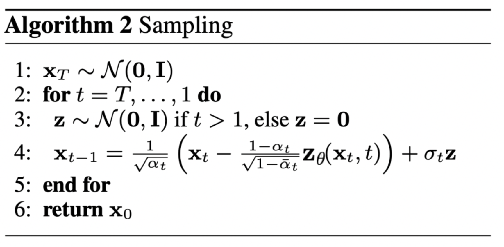
Generating new images from a diffusion model happens by reversing the diffusion process: we start from , where we sample pure noise from a Gaussian distribution, and then use our neural network to gradually denoise it (using the conditional probability it has learned), until we end up at time step . As shown above, we can derive a slighly less denoised image by plugging in the reparametrization of the mean, using our noise predictor. Remember that the variance is known ahead of time.
Ideally, we end up with an image that looks like it came from the real data distribution.
The code below implements this.
@torch.no_grad()
def p_sample(model, x, t, t_index):
    betas_t = extract(betas, t, x.shape)
    sqrt_one_minus_alphas_cumprod_t = extract(
        sqrt_one_minus_alphas_cumprod, t, x.shape
    )
    sqrt_recip_alphas_t = extract(sqrt_recip_alphas, t, x.shape)

    # Equation 11 in the paper
    # Use our model (noise predictor) to predict the mean
    model_mean = sqrt_recip_alphas_t * (
        x - betas_t * model(x, t) / sqrt_one_minus_alphas_cumprod_t
    )

    if t_index == 0:
        return model_mean
    else:
        posterior_variance_t = extract(posterior_variance, t, x.shape)
        noise = torch.randn_like(x)
        # Algorithm 2 line 4:
        return model_mean + torch.sqrt(posterior_variance_t) * noise

# Algorithm 2 (including returning all images)
@torch.no_grad()
def p_sample_loop(model, shape):
    device = next(model.parameters()).device

    b = shape[0]
    # start from pure noise (for each example in the batch)
    img = torch.randn(shape, device=device)
    imgs = []

    for i in tqdm(reversed(range(0, timesteps)), desc='sampling loop time step', total=timesteps):
        img = p_sample(model, img, torch.full((b,), i, device=device, dtype=torch.long), i)
        imgs.append(img.cpu().numpy())
    return imgs

@torch.no_grad()
def sample(model, image_size, batch_size=16, channels=3):
    return p_sample_loop(model, shape=(batch_size, channels, image_size, image_size))
Note that the code above is a simplified version of the original implementation. We found our simplification (which is in line with Algorithm 2 in the paper) to work just as well as the original, more complex implementation, which employs clipping.
Train the model
Next, we train the model in regular PyTorch fashion. We also define some logic to periodically save generated images, using the sample method defined above.
from pathlib import Path

def num_to_groups(num, divisor):
    groups = num // divisor
    remainder = num % divisor
    arr = [divisor] * groups
    if remainder > 0:
        arr.append(remainder)
    return arr

results_folder = Path("./results")
results_folder.mkdir(exist_ok = True)
save_and_sample_every = 1000
Below, we define the model, and move it to the GPU. We also define a standard optimizer (Adam).
from torch.optim import Adam

device = "cuda" if torch.cuda.is_available() else "cpu"

model = Unet(
    dim=image_size,
    channels=channels,
    dim_mults=(1, 2, 4,)
)
model.to(device)

optimizer = Adam(model.parameters(), lr=1e-3)
Let's start training!
from torchvision.utils import save_image

epochs = 6

for epoch in range(epochs):
    for step, batch in enumerate(dataloader):
      optimizer.zero_grad()

      batch_size = batch["pixel_values"].shape[0]
      batch = batch["pixel_values"].to(device)

      # Algorithm 1 line 3: sample t uniformally for every example in the batch
      t = torch.randint(0, timesteps, (batch_size,), device=device).long()

      loss = p_losses(model, batch, t, loss_type="huber")

      if step % 100 == 0:
        print("Loss:", loss.item())

      loss.backward()
      optimizer.step()

      # save generated images
      if step != 0 and step % save_and_sample_every == 0:
        milestone = step // save_and_sample_every
        batches = num_to_groups(4, batch_size)
        all_images_list = list(map(lambda n: sample(model, batch_size=n, channels=channels), batches))
        all_images = torch.cat(all_images_list, dim=0)
        all_images = (all_images + 1) * 0.5
        save_image(all_images, str(results_folder / f'sample-{milestone}.png'), nrow = 6)
Output:
----------------------------------------------------------------------------------------------------
Loss: 0.46477368474006653
Loss: 0.12143351882696152
Loss: 0.08106148988008499
Loss: 0.0801810547709465
Loss: 0.06122320517897606
Loss: 0.06310459971427917
Loss: 0.05681884288787842
Loss: 0.05729678273200989
Loss: 0.05497899278998375
Loss: 0.04439849033951759
Loss: 0.05415581166744232
Loss: 0.06020551547408104
Loss: 0.046830907464027405
Loss: 0.051029372960329056
Loss: 0.0478244312107563
Loss: 0.046767622232437134
Loss: 0.04305662214756012
Loss: 0.05216279625892639
Loss: 0.04748568311333656
Loss: 0.05107741802930832
Loss: 0.04588869959115982
Loss: 0.043014321476221085
Loss: 0.046371955424547195
Loss: 0.04952816292643547
Loss: 0.04472338408231735
Sampling (inference)
To sample from the model, we can just use our sample function defined above:
# sample 64 images
samples = sample(model, image_size=image_size, batch_size=64, channels=channels)

# show a random one
random_index = 5
plt.imshow(samples[-1][random_index].reshape(image_size, image_size, channels), cmap="gray")
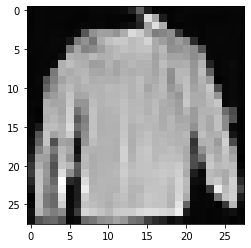
Seems like the model is capable of generating a nice T-shirt! Keep in mind that the dataset we trained on is pretty low-resolution (28x28).
We can also create a gif of the denoising process:
import matplotlib.animation as animation

random_index = 53

fig = plt.figure()
ims = []
for i in range(timesteps):
    im = plt.imshow(samples[i][random_index].reshape(image_size, image_size, channels), cmap="gray", animated=True)
    ims.append([im])

animate = animation.ArtistAnimation(fig, ims, interval=50, blit=True, repeat_delay=1000)
animate.save('diffusion.gif')
plt.show()

Follow-up reads
Note that the DDPM paper showed that diffusion models are a promising direction for (un)conditional image generation. This has since then (immensely) been improved, most notably for text-conditional image generation. Below, we list some important (but far from exhaustive) follow-up works:
- Improved Denoising Diffusion Probabilistic Models (Nichol et al., 2021): finds that learning the variance of the conditional distribution (besides the mean) helps in improving performance
- Cascaded Diffusion Models for High Fidelity Image Generation (Ho et al., 2021): introduces cascaded diffusion, which comprises a pipeline of multiple diffusion models that generate images of increasing resolution for high-fidelity image synthesis
- Diffusion Models Beat GANs on Image Synthesis (Dhariwal et al., 2021): show that diffusion models can achieve image sample quality superior to the current state-of-the-art generative models by improving the U-Net architecture, as well as introducing classifier guidance
- Classifier-Free Diffusion Guidance (Ho et al., 2021): shows that you don't need a classifier for guiding a diffusion model by jointly training a conditional and an unconditional diffusion model with a single neural network
- Hierarchical Text-Conditional Image Generation with CLIP Latents (DALL-E 2) (Ramesh et al., 2022): uses a prior to turn a text caption into a CLIP image embedding, after which a diffusion model decodes it into an image
- Photorealistic Text-to-Image Diffusion Models with Deep Language Understanding (ImageGen) (Saharia et al., 2022): shows that combining a large pre-trained language model (e.g. T5) with cascaded diffusion works well for text-to-image synthesis
Note that this list only includes important works until the time of writing, which is June 7th, 2022.
For now, it seems that the main (perhaps only) disadvantage of diffusion models is that they require multiple forward passes to generate an image (which is not the case for generative models like GANs). However, there's research going on that enables high-fidelity generation in as few as 10 denoising steps.